HAL Id: insu-00987388
https://hal-insu.archives-ouvertes.fr/insu-00987388
Submitted on 16 May 2014HAL is a multi-disciplinary open access archive for the deposit and dissemination of sci-entific research documents, whether they are pub-lished or not. The documents may come from teaching and research institutions in France or abroad, or from public or private research centers.
L’archive ouverte pluridisciplinaire HAL, est destinée au dépôt et à la diffusion de documents scientifiques de niveau recherche, publiés ou non, émanant des établissements d’enseignement et de recherche français ou étrangers, des laboratoires publics ou privés.
The electrical conductivity during incipient melting in
the oceanic low-velocity zone
David Sifré, Emmanuel Gardès, Malcolm Massuyeau, Leila Hashim, Saswata
Hier-Majumder, Fabrice Gaillard
To cite this version:
David Sifré, Emmanuel Gardès, Malcolm Massuyeau, Leila Hashim, Saswata Hier-Majumder, et al.. The electrical conductivity during incipient melting in the oceanic low-velocity zone. Nature, Nature Publishing Group, 2014, 509, pp.81-85. �10.1038/nature13245�. �insu-00987388�
1
The electrical conductivity during incipient melting in the oceanic low velocity
zone.
David Sifré1,2,3, Emmanuel Gardés1,2,3,4, Malcolm Massuyeau1,2,3, Leila Hashim1,2,3, Saswata Hier-Majumder1,2,3,5,6, Fabrice Gaillard1,2,3.
1Université d’Orléans, ISTO, UMR 7327, 45071 Orléans, France. 2
CNRS/INSU, ISTO, UMR 7327, 45071 Orléans, France.
3
BRGM, ISTO, UMR 7327, BP 36009, 45060 Orléans, France.
4
CEA-CNRS-ENSICAEN-Université de Caen Basse Normandie, CIMAP, UMR 6252, BP 5133, 14070 Caen, France.
5
Department of Geology and CSCAMM,University of Maryland, MD 20742, USA.
6
Dept. of Earth Sciences, Royal Holloway University of London Egham, Surrey, UK.
A low viscosity layer in the upper mantle, the Asthenosphere, is a requirement for plate tectonics1. The seismic low velocities and the high electrical conductivities of the Asthenosphere are attributed either to sub-solidus water-related defects in olivine minerals2-4 or to a few volume percents of partial melt5-8 but these two interpretations have shortcomings: (1) The amount of H2O stored in olivine is not expected to be higher than 50
ppm due to partitioning with other mantle phases9, including pargasite amphibole at moderate temperatures10, and partial melting at high temperatures9; (2) elevated melt volume fractions are impeded by the too cold temperatures prevailing in the Asthenosphere and by the high melt mobility that can lead to gravitational segregation11,12. Here we determined the electrical conductivity of CO2-H2O-rich melts, typically produced at the
onset of mantle melting. Electrical conductivity modestly increases with moderate amounts of H2O and CO2 but it dramatically increases as CO2 content exceeds 6 wt% in the melt.
Incipient melts, long-expected to prevail in the asthenosphere10,13-15, can therefore trigger its high electrical conductivities. Considering depleted and enriched mantle abundances in H2O and CO2 and their effect on the petrology of incipient melting, we calculated
conductivity profiles across the Asthenosphere for various plate ages. Several electrical discontinuities are predicted and match geophysical observations in a consistent petrological and geochemical framework. Below moderately aged plates (>5Ma), incipient melts most likely trigger both the seismic low velocities and the high electrical conductivities in the upper part of the asthenosphere; whereas beneath young plates4, on top of which, seamount volcanism occurs, higher degree of melting is expected to cause high conductivities6.
2
The lithosphere is a chemically depleted and mechanically strong region of the uppermost mantle, overlying the chemically enriched and mechanically weak asthenosphere 1-3,8,16. Volatile enrichments in the asthenosphere have long been shown to trigger incipient melting10,13-15 (that is small degree of partial melting due to small amounts of CO2 and H2O) in the upper part of the
asthenosphere and a link between incipient melting and seismic low velocity zone has also long been suggested13,15,17. In this article, we demonstrate that incipient melting of the mantle by the presence of small amounts of CO2 and H2O can also trigger high electrical conductivities. We
herein assume that the low viscosity layer, the high electrical conductivity layer (ECL) and low seismic velocity layer (LVZ) are coincident, and use the term Asthenosphere for this layer.
The Asthenosphere is characterized by high electrical conductivities4,5,18 and reduced S-wave velocities8,16. While the characteristics of the Asthenosphere are commonly related to water related defects in olivine2-4, a number of multidisciplinary observations5-8,10,13,15,17-20 and the discovery of petit spot volcanoes21 indicate that the Asthenosphere most likely contains partial melt.
Two issues arise when the observed features of the Asthenosphere are attributed to partial melting: (1) a few volume percentages of basaltic melt are generally required to explain high electrical conductivities, which is problematic as melt would unavoidably tend to rise if present at such high amounts11-12 and (2) the lithosphere-asthenosphere boundary (LAB) occurs at a near constant depth of 50-75 km for both warm/young and cold/ancient lithospheres4,5,8,16,18, where the temperature may not be sufficiently high to produce such amounts of melt.
However, incipient CO2-H2O rich melts, that are stable under the P-T-fO2 conditions of the
Asthenosphere10,13-15,17,22-23, allow melting in both warm and cold regions of the Asthenosphere17. Low temperature carbonatite melts, composed of almost 50% CO2, are characterized by high
electrical conductivities19, but their stability is restricted to the coldest and driest regions of the Asthenosphere17. Increasing temperature or water content changes the composition of the prevailing melts to intermediates between basalts and carbonatites, often described as carbonated basalts17,22. Very little is known about the physical properties of such intermediate volatile-rich melts (CO2 and H2O). In particular, their electrical properties have never been measured. In order
to address the issues regarding onset of partial melting at the LAB, and to permit a test of the incipient melting model suggested by petrological studies15,17, we performed electrical conductivity measurements on CO2-H2O-rich melts.
We developed a new experimental set-up, specifically adapted for liquids with high conductivities (Fig. SI1). The high performance of this modified 4-wire method, adapted to ½ inches piston cylinders, is discussed in the Methods section and figures SI2-SI5. Five melts, with CO2 and H2O contents ranging from 10 to 48 wt% and 0 to 10 wt%, respectively, were analysed
by impedance spectroscopy in the temperature range 900 - 1500°C at a confining pressure of 3 GPa. We tested the reproducibility of the measurements by taking measurements during both cooling and heating of the samples (Fig. SI5) and we verified that decarbonation and dehydration
3
of samples at high temperature did not affect the conductivity results. Figure 1 reports the measured electrical conductivities as a function of reciprocal temperature. For similar water contents, the electrical conductivity of carbonated basalts is higher than that of hydrated basalts and the difference increases with an increase in the CO2 content of the melt to a maximum of
nearly one log unit. The most CO2-rich melt has conductivities higher than 200 S.m-1. We
develop a semi-empirical law that takes into account the two parallel conductive processes operating in carbonated basalts: conduction by covalent polymer-like hydrous silicate melts and ionic conduction by carbonate melts19.
( (
)) (
(
)) (1)
The calculated conductivities using equation 1, as shown in figure 1, reproduce our measurements and those of ref. 7 on CO2-free hydrated basalts with an average precision of 5%
in seeMethods). The effect of CO2 on melt conductivity, predicted by equation 1, is negligible
at low CO2 content, but increases sharply for CO2 content higher than 6 wt%. Such a change is
most likely caused by an abrupt transition in the melt structure and properties from silicate-type to carbonate-type.
We calculate the mantle electrical conductivity for variable amounts of bulk H2O and CO2
contents in a partially molten peridotite. We assume that the interconnected melt is equally distributed between grain edge tubules and grain boundary melt films18,20,24 (see Methods). The conductivity of hydrated olivine was calculated from ref. 25 and equation 1 was used for CO2
-H2O-bearing melts. We assume that carbon is exclusively soluble in the melt23 (carbonate units)
and computed the partitioning of water between carbonated melt, pargasite, olivine, and peridotite combining ref. 9, 10 and 22. We report results for partially molten peridotite containing only H2O (Fig. 2A) and both CO2 and H2O (Fig. 2B and 2C). In all simulations, partitioning
constraints for CO2 and H2O between solids and melts impose that (1) CO2-H2O-rich melts can
only be produced at the onset of mantle partial melting and (2) that small melt fractions always contain far more CO2 than H2O (see top axis in fig.2). If > 1% melting is attained, the melt
volatile contents drop to values that modestly impacts on their electrical conductivity.
The CO2-free depleted mantle, containing ca. 200 ppm H2O26-28, cannot be conductive at
temperatures below 1350°C (i.e. ≥ 0.1 S.m-1), unless it contains more than ~5 vol.% basaltic melts (Fig. 2A). Only unreasonably high temperatures for the LAB (>1450°C) can make the mantle conductive with small amounts of melt (<1 vol%). Moreover, at high melt percentage, water has almost no effect on mantle conductivity, since its content in the melt remains small (i.e. <1 wt% H2O negligibly affects basalt conductivity). If an enriched mantle is considered (500
ppm H2O), a reasonably low melt content (1 vol.%) can trigger high conductivity but it still
4
In presence of CO2, the formation of incipient CO2-rich melts (<0.5 vol.%) disproportionately
increases the effective electrical conductivity of the mantle (Fig. 2B and 2C). For example, in the depleted mantle, containing 200 ppm H2O and 200 ppm CO226 and fuelling the dominant part of
MORBs27-28, 0.1-0.15 vol.% of melt at 1325°C can explain the high electrical conductivity of the ECL reported in oceanic domains5,18,29. The melt is a carbonated basalt, typically containing 15-35 wt% CO2 and about 2-3 wt% H2O (Fig.2B). Remarkably, the enriched mantle27-28 with 500
ppm H2O and 500 ppm CO2 can produce high conductivities at temperature and melt fractions as
low as 1050°C and 0.2 vol%. We also notice that incipient melting of the enriched mantle triggers conductivities that are 2.5 times greater than the depleted mantle making variations in electrical conductivity a powerful probe of the chemical enrichment in the upper mantle.
The stability of incipient melts in the upper part of the asthenosphere has long been shown by petrological constraints13-15, that are not considered in Fig. 2. The P-T region of incipient melting in peridotite is shown in Fig. SI8 together with the stability domain of pargasite, that is the main solid host for water in peridotite containing more than 150-200 ppm10. We calculate that the presence of pargasite restricts the amount of water to 40-50 ppm in olivine, according to partition coefficient among peridotite minerals9,10. Pargasite is however unstable at T>1070°C10 and its occurrence must be merely considered for the enriched mantle (>200 ppm H2O). Based on the
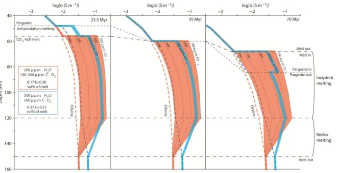
P-T phase diagram of Fig. SI8 and considering oceanic geotherms at 23.5, 35 and 70 Ma, we have calculated 1D conductivity profiles illustrating the impact of several petrological discontinuities (Fig. 3). We have considered the depleted mantle (200 ppm H2O plus CO2 varying from 100 to
500 ppm) and the enriched mantle (500 ppm H2O and 500 ppm CO2). Variable CO2 contents in
the depleted mantle account for the fact that MORBs have degassed their CO2 and the carbon
content of their source is therefore highly uncertain26-28.
The upper discontinuity (Fig. 3) predicted by our model is the beginning of incipient melting at ~50 km depth for young/warm plates and at ~70 km for colder/older plates. This discontinuity marks the thermodynamic boundary between CO2-rich melt and CO2-rich vapour14: the melt
being stable at greater depth. In the case of an enriched mantle, an additional discontinuity occurs due to the pargasite dehydration melting reaction (producing CO2-H2O rich, low SiO2 melt) that
can be shallower than the previously described discontinuity for young plates (ie. 23.5Ma) and deeper for old plates (70 Ma). At 35 Ma, these two discontinuities occur at the same depth (60 km). The lowest discontinuity shown in Fig. 3 occurs in the depth interval 120-150 km and is described as the region of redox melting22,23; that is the boundary separating diamonds from CO2
-rich melts, the melt being stable at shallower depth. Incipient melting, which triggers the conductive region of the asthenosphere, is therefore permitted between the redox melting lower boundary and the decarbonation upper boundary and this agrees well with electromagnetic observations in oceanic domains4,5,18,22,29, though ref. (29) indicates slightly deeper ranges.
The increase in conductivity in the incipient melting region is major, being half a log-unit for the depleted mantle (200 ppm CO2) and more than one log-unit for the mantle containing 500 ppm
5
in the case of young plates. Note that the surprising effect of water (Fig. 3), where incipient melting in a mantle with 500 ppm H2O and 500 ppm CO2 induces lower conductivities than in a
mantle with 200 ppm H2O the same amount of CO2. The imaging of the 23.5 Ma old LAB by ref.
5 at ~50 km depth revealed conductivities of 0.1-0.2 S.m-1. These are definitely not explainable by melting of a CO2-free H2O-depleted mantle, since too high temperatures and/or too high melt
contents are demanded (Fig. 2). They cannot be explained by pargasite dehydration melting in a CO2-free H2O-enriched mantle either, as this process cannot produce high enough conductivities
(Fig. 3, Fig. SI9). Once deciphered in a petrological framework, the conductivities of the LAB in ref. 5 can be reached by incipient melting of a mantle containing 400 ppm CO2 (Fig. 3). We recall
that ref. 5 introduced moderate electrical anisotropy in the inversion of their magnetotelluric data whereas we merely discuss here the geometric mean conductivity, which is much less model dependent.
The presence of CO2-rich melts in the asthenosphere not only better explains the electrical
properties of the Asthenosphere, but also explains the weak dependence of the lithosphere thickness on the age of the oceanic crust (Fig. 4). The bottom of the lithosphere in Fig. 4 marks a seismic discontinuity characterised by a reduction in S-waves velocity of 5 to 15 %8,16. This discontinuity cannot be caused by partial melting of a dry or water under-saturated mantle, as this may only occur at higher depths and temperatures9 (see blue melting curve on Fig. 4). Previously suggested melting reactions such as the dehydration melting of amphibole10 also fail to reproduce the depth-age relationships of the LAB (Fig. 4). Remarkably, the CO2+H2O melting curve14,
which delimits the upper boundary of the incipient melting region already shown in Fig. 3, ranges from 50 km down to 80 km depths from the youngest to the oldest lithospheres (purple curve in Fig. 4). This correlates pretty well with the bottom of the lithosphere as imaged by the seismic discontinuity. The lower limit of incipient melting, i.e. the redox melting22,23, matches also well the lower part of the seismic low velocity zone8 at depth of about 140-180 km. At low pressures, above the incipient melting region, the decarbonation of the melt forms an impermeable layer in which buoyant CO2-rich melts are frozen into clinopyroxene-rich residue (with pargasite) and
CO2-rich fluids (Fig.4). Melting is therefore permitted in the Asthenosphere and the melt cannot
rise through the LAB because of the existence of this melt-freezing boundary (see Methods). It is only where the mantle is hot enough to suppress the freezing reaction (that is melting does not anymore require CO2) and where melt fractions are large enough12 (2-5 vol%) that melts can rise
to the LAB. This occurs for young plates (<5Ma), where volcanic seamounts are observed, and this has also been related6 to the electrical properties of the young LAB4.
Incipient melting has long been described as a key petrological process operating in the seismic low velocity region marking the upper asthenosphere13,15,17. The mantle geochemistry and petrology in this region argues for production of incipient CO2-enriched melts9,10,13,15. We
demonstrate that these melts have conductivities of hundreds of S/m, much higher than CO2-free
hydrated melts or hydrated minerals. Our modelling, despite unavoidable simplifications, considers geochemical and petrological constraints and indicates that mantle with small fractions
6
of CO2-rich melts at 50-150 km reproduces the electrical properties as well as the depth of the
LAB pretty well, whereas CO2-free systems yields too poor or no agreement with geophysical
observations. The presence of CO2-rich incipient melts in the Asthenosphere has important
implications for radiogenic heat production as such melts are enriched in heat-producing elements like K-U-Th30. Moreover, the involvement of CO2-rich incipient melts is also
recognized in petrological processes occurring in the continental and in the cratonic LAB30. The Asthenosphere - incipient melting association we suggest here can therefore be extended to geodynamic settings other than the oceanic domains. It remains however to be defined how the mechanical strength of the Asthenosphere can be impacted by small amount of CO2-H2O-rich
melts and how this can be connected to plate motions.
METHODS SUMMARY
Starting materials were mixtures of basaltic glass and hydrated Ca-Mg-Carbonates, so that water and CO2 were all together introduced in our sample with a constant molar CO2/H2O ratio of 2 (in
mole; see Table SI1). Two dry carbonate melts were also investigated. The extent of dehydration and decarbonation of our samples during high temperature-high pressure experiments were shown to be small (Table SI1 vs. SI2). The effect of H2O was disentangled from that of CO2 by
using published experimental conductivity measurements on hydrated basalts7 and the empirical equation 1. This empirical simplification is in line with the effect of water on the conductivity of carbonated melts that we determined here (circles vs. squares in Fig. SI5): it is moderate and almost similar to that recently determined for basalts7. Equation 1 was used for simulations in Fig. 2 and Fig. 3 remaining within the range of experimentally investigated H2O and CO2
contents.
Figures 2 and 3 have been constructed considering that incipient melts are well connected20,24. Ref. 24 constitutes the only work specifically tackling the connectivity of incipient carbonated melts in olivine and it shows interconnection at the small melt fractions we are considering. Ref. 20 confirmed the good connection for melt contents of ~1%. Mixtures of melt tubes and melt films have been considered in our plots; the difference between both geometries implies conductivities differing by ca. 0.2 log-units.
The isotherms in figure 4 were obtained considering the sudden half space cooling model with similar parameters as in ref. 8. The use of more complicated models such as the plate model (see ref. 17, which is, conversely to us, a priori deciding for a thickness of the lithosphere) yields similar isotherms8 for the moderate depths we discuss here.
7
1. Höink, T., Jellinek, A.M. & Lenardic, A. Viscous coupling at the lithosphere-asthenosphere boundary.Geochem.Geophys. Geosyst. 12, Q0AK02 (2011).
2. Hirth, G. & Kohlstedt, D.L. Water in the oceanic upper mantle: Implications for rheology, melt extraction and the evolution of the lithosphere. Earth Planet. Sci. Lett. 144, 93-108 (1996). 3. Karato, S. On the origin of the asthenosphere. Earth Planet. Sci. Lett. 321, 95-103 (2012). 4. Evans, R.L., Hirth, G., Baba, K., Forsyth, D., Chave, A. & Mackie, R. Geophysical evidence from the MELT area for compositional controls on oceanic plates. Nature 437, 249-252 (2005).
5. Naif, S., Key, K., Constable, S. & Evans, R.L. Melt-rich channel observed at the lithosphere-asthenosphere boundary, Nature 495, 356-359 (2013).
6. Caricchi, L., Gaillard, F., Mecklenburgh, J. & Le Trong E. Experimental determination of electrical conductivity during deformation of melt-bearing olivine aggregates: Implications for electrical anisotropy in the oceanic low velocity zone. Earth Planet. Sci. Lett. 302, 81-94 (2011). 7. Ni, H., Keppler, H. & Behrens, H. Electrical conductivity of hydrous basaltic melts: implications for partial melting in the upper mantle. Contrib. Mineral. Petrol. 162, 637–650 (2011).
8. Schmerr, N. The Gutenberg discontinuity: melt at the lithosphere-asthenosphere boundary. Science 335, 1480-1483 (2012).
9. Hirschmann, M., Tenner, T., Aubaud, C. & Withers, A.C. Dehydration melting of nominally anhydrous mantle: The primacy of partitioning. Phys. Earth Planet. Inter. 176, 54-68 (2009).
10. Green, D.H., Hibberson, W.O., Kovács, I. & Rosenthal, A. Water and its influence on the lithosphere-asthenosphere boundary. Nature 467, 448-U97 (2010).
11. Hier-majumder, S., Courtier, A. Seismic signature of small melt fraction atop the transition zone. Earth Planet. Sci. Lett. 308, 334–342 (2011). doi:10.1016/j.epsl.2011.05.055. 12. Faul, U. H., Melt retention and segregation beneath mid-ocean ridges. Nature 410, 920–3 (2001). doi:10.1038/35073556.
13. Presnall, D.C. & Gudfinnsson, G.H. Carbonate-rich melts in the oceanic low-velocity zone and deep mantle. Geol. Society of America, Special Papers 388, 207-216 (2005).
14. Wallace, M.E. & Green, D.H. An experimental determination of primary carbonatite magma composition. Nature 335, 343-346 (1988)
15. Green, D.H., Liebermann, R.C, Phase-equilibra and elastic properties of a pyrolite model for oceanic upper mantle, Tectonophysics 32, 61-92 (1976)
16. Fischer, K.M., Ford, H.A., Abt, D.L. & Rychert, C.A. The Lithosphere-Asthenosphere Boundary. Annual Review of Earth and Planetary Sciences 38, 551-575 (2010).
8
17. Hirschmann, M.M. Partial melt in the oceanic low velocity zone. Phys. Earth Planet.
Inter. 179, 60–71 (2010).
18. Utada, H., Baba, K., Estimating the electrical conductivity of the melt phase of a partially molten asthenosphere from seafloor magnetotelluric sounding data, Physics of the Earth and
Planetary Interiors (2013), doi: http://dx.doi.org/10.1016/j.pepi.2013.12.004.
19. Gaillard, F., Malki, M., Iacono-Marziano, G., Pichavant, M. & Scaillet, B. Carbonatite melts and electrical conductivity in the asthenosphere. Science 322, 1363-1365 (2008).
20. Yoshino, T., Laumonier, M., McIsaac, E. & Katsura, T. Electrical conductivity of basaltic and carbonatite melt-bearing peridotites at high pressures: Implications for melt distribution and melt fraction in the upper mantle. Earth Planet. Sci. Lett. 295, 593–602. (2010).
21. Hirano, N., Takahashi, E., Yamamoto, J. et al. Volcanism in Response to Plate Flexure.
Science 313, 1426-1428 (2006).
22. Dasgupta, R., Mallik, A., Tsuno, K., Withers, A.C., Hirth, G. & Hirschmann, M.M. Carbon-dioxide-rich silicate melt in the Earth's upper mantle. Nature 493, 211-U222 (2013). 23. Stagno, V., Ojwang, D.O., McCammon, C.A. & Frost, D.J. The oxidation state of the mantle and the extraction of carbon from Earth's interior. Nature 493, 84 (2013).
24. Minarik, W.G. & Watson, E.B. Interconnectivity of carbonate melt at low melt fraction.
Earth Planet. Sci. Lett. 133, 423-437 (1995).
25. Jones, A. G., Fullea, J., Evans, R. L., Muller, M.R. Water in cratonic lithosphere: Calibrating laboratory determined models of electrical conductivity of mantle minerals using geophysical and petrological observations. Geochem. Geophys. Geosyst. 13, Q06010 (2012) 26. Cartigny, P., Pineau, F., Aubaud, C. & Javoy, M. Towards a consistent mantle carbon flux estimate: Insights from volatile systematics (H2O/Ce, δD, CO2/Nb) in the North Atlantic mantle (14° N and 34° N). Earth Planet. Sci. Lett. 265, 672–685 (2008).
27. Marty B., The origins and concentrations of water, carbon, nitrogen and noble gases on Earth. Earth Planet. Sci. Lett. 313-314, 56–66 (2012).
28. Dasgupta, R., Hirschmann, M.M., The deep carbon cycle and melting in Earth's interior.
Earth Planet. Sci. Lett. 298, 1–13 (2010)
29. Lizarralde, D., Chave, A., Hirth, G., Schultz, A., Northeastern Pacific mantle conductivity profile from long-period magnetotelluric sounding using Hawaii-to-California submarine cable data. J. Geophys. Res., 100(B9), 17837–17854 (1995).
30. O’Reilly, S.Y. & Griffin, W.L. The continental lithosphere-asthenosphere boundary: Can we sample it? Lithos 120, 1-13 (2010).
9
Supplementary information (9 figures, 5 Tables)
Acknowledgments- This work, part of the ElectroLith project, benefited from funding by the
European Research Council (ERC project #279790) and the French agency for research (ANR project # 2010 BLAN62101). SH-M acknowledges support from the NSF grant EAR1215800 and a grant from the University of Orléans.
Authors contributions- F.G. is leading the project and wrote the first draft. All authors equally
contributed to the writing. D.S. and F.G. developed the experimental setup and D.S. performed the conductivity measurements. S.H-M contributed to the discussion and provided editorial assistance with manuscript. D.S. and L.H. did figure 1, E.G. and L.H. did figure 2, D.S. did figure 3 and L.H., M.M. did figure 4.
METHODS: Starting materials
Electrical measurements were performed on five mixtures: 2 dry carbonated melts (CO2=44
-48wt%), a hydrous carbonated melt (CO2 =25.9 wt%; H2O=10.2 wt%) and 3 hydrous carbonated
basalts (CO2 = 10.39 to 23.32 wt%; H2O=4.43 to 9.22 wt.%, Table SI1). Starting materials used
to obtain these mixtures were natural dolomite (MgCa(CO3)2), a natural basalt (popping rock31),
salt (NaCl), sodium carbonates (Na2CO3) and brucite (Mg(OH)2) (Table SI1).
Experiments
All experiments were performed at 3 GPa in ½-inches piston cylinders (graphite-Pyrex-talc assemblages), which was connected to a 1260 Solartron Impedance/Gain Phase Analyzer for electrical conductivity measurements. The temperature was measured with a B-type thermocouple localized on sample top (Fig. SI1). Oxygen fugacity (fO2) was not controlled
during the measurements but the presence of graphite (furnace) and molten carbonates (sample) should imply an oxygen fugacity close to FMQ-223.
We have developed a new protocol specifically adapted for electrical conductivity measurements on highly conductive and molten materials (Fig. SI1). The new design employs a pseudo-4-wire configuration, which removes the electrical contribution of the electrical cell itself (Fig. SI2). Such a configuration previously adapted at 1 atm19,32 is here shown necessary for measurements on H2O-CO2-rich melts at 3 GPa.
Cold pressed pellets (5 mm outer diameter) were cored in their centre in order to place an inner Pt electrode (1 mm). A Pt foil surrounding the cylindrical sample was used as outer electrode. An alumina jacket isolated the entire electrical cell from the graphite furnace. The sample impedance was measured between the two electrodes arranged in a co-axial geometry33,34. The inner electrode was connected to the impedance spectrometer via the two wires of the thermocouple34. The outer electrode was connected to a nickel cylinder (located 5 mm above the sample) that was mounted in series with two additional wires (B-type thermocouples) (Fig. SI1).
Data reductions and uncertainties
The electrical conductivities of the samples were calculated from the measured resistances using the following relationship33,34:
10
⁄
(2)
with σ being the electrical conductivity in S.m-1, rout, rin, h, respectively the outer radius, the inner
radius and the height of the samples in m, and R, the resistance of the sample in Ω (Fig. SI3 and SI4).
Uncertainties in were calculated as a function of geometrical factors of the samples (Fig. SI4) and propagating errors of each measured resistance. The uncertainties on are 7 % on average for all measurements and reach a maximum of 16% on HCB-4.
Sample characterization
Scanning electron microscope (SEM) imaging and electron microprobe analyses (EMPA) were systematically operated after each experiment. Determination of rout, rin and h by SEM imaging
showed an average decrease of 20% compared to the initial geometry, most likely due to porosity loss during melting (Fig. SI4). No melt leak was observed and the entire sample remained sandwiched between the MgO plugs and the electrodes.
EMP analyses were conducted at 15 KeV, 10 nA and 10 sec counting on peak elements. The beam size (100 μm x 100 μm) was adapted to obtain average chemical compositions, smoothing the heterogeneities due to quench crystallizations. Comparison of compositions before and after experiments shows no contamination by the MgO surrounding the sample and no considerable volatile loss from the sample to the surrounding assemblages (Tables SI1, SI2). CO2 content were
determined using the by-difference method22 and indicate negligible decarbonation.
An elemental analyser, type Flash 2000 (Thermo Scientific; see SI), was used to measure H2O
content of sample (before and) after experiments. Samples are heated to >1500°C and the released H2O is reduced into elemental H being finally detected by a highly sensitive thermal
conductivity detector. This gives water content with a precision of +/- 0.5 wt%. We observed a negligible dehydration during conductivity measurements.
Conductivity Results and Modelling
Figure SI5 shows the good reproducibility of the electrical measurements during heating and cooling cycles. The conductivity-temperature relationships for each sample were fitted using an Arrhenius law and the calculated pre-exponential factors and activation energies are presented in Table SI4.
In the semi-empirical law (equation 1), the pre-exponential factor 0 and the activation energy Ea
for both H2O and CO2 terms are related by a compensation law35,36 (Fig. SI5)
( ) (3)
the decrease of activation energy as a function of volatile content is exponential
( ) (4)
Cvolatile is the CO2 and H2O content in wt%. The optimized parameters a, b, c, d and e are given in
Table SI5 together with their propagated uncertainties. Our model reproduces the experimental measurements on within an average error of 5% (maximum 10%).
11
The bulk rock is considered as a peridotite containing a fraction of interconnected melt, where volatiles partition between the solid and the melt phase. The bulk H2O content is related to H2O
in melt and in peridotite as:
( ) ⁄ and ⁄ ( ) ⁄ (5)
where is the mass fraction of melt and ⁄ is the partition coefficient of H2O
between peridotite and melt (0.007, i.e. average partition coefficient over 1.5-4 GPa9,37). We assume that CO2 distributes exclusively in the liquid phase23,38, i.e. ⁄ .
Conversion from mass to volume fraction of melt is done considering volume properties of silicate melts39 and carbonate melts40,41. The conductivity of the melt ( ) was
calculated using equation 1. The conductivity of the peridotite was assumed to be controlled by that of hydrous olivine25.
The bulk conductivity was calculated using the mean of tube42-44 and film44-47 geometries resulting in values almost similar to refs (20, 46).
Melt fraction in Fig. 3 was approximated as48 = 2.5×CO2bulk + 6×H2Obulk.
Buoyant basalts versus incipient melts
An impermeable layer has been suggested to limit or prevent the melt prevailing in the LAB from rising to the surface49. The rate of melt ascent due to buoyancy is otherwise expected to be of the order of several cm/year11,12, if melt content is 3-5 vol. %. Our model of incipient melting implies an impermeable boundary that is caused by phase relationships14, i.e. a thermodynamic boundary through which melt cannot rise. We furthermore emphasise the limited melt mobility50 at the small melt fraction of interest as, in particular, surface tensions would unavoidably tend to retain the buoyant melt51. To conclude, if basalts, being anyway not thermodynamically stable in the asthenosphere, tend to migrate out of the asthenosphere52, small melt fractions may in contrast be mechanically stable in the LAB.
ADDITIONAL REFERENCES FOR METHODS:
31. Javoy, M. & Pineau, F. The volatiles record of a "popping" rock from the Mid-Atlantic Ridge at 14 ° N: chemical and isotopic composition of gas trapped in the vesicles. Earth Planet.
Sci. Lett. 107, 598-611 (1991).
32. Pommier, A., Gaillard, F., Malki, M. & Pichavant, M. Methodological re-evaluation of the electrical conductivity of silicate melts. Am. Mineral. 95, 284-291 (2010).
33. Gaillard, F. Laboratory measurements of electrical conductivity of hydrous and dry silicic melts under pressure. Earth Planet. Sci. Lett. 218, 215-228 (2004).
12
34. Hashim, L., Gaillard, F., Champallier, R., Le Breton, N., Arbaret, L., Scaillet, B. Experimental assessment of the relationships between electrical resistivity, crustal melting and strain localization beneath the Himalayan-Tibetan belt. Earth Planet. Sci. Lett. 373, 20-30 (2013) doi:10.1016/j.epsl.2013.04.026.
35. Pommier, A., Gaillard, F., Pichavant, M. & Scaillet, B. Laboratory measurements of electrical conductivities of hydrous and dry Mount Vesuvius melts under pressure. J. Geophys.
Res. Solid Earth 113, B05205 (2008).
36. Tyburczy, J. & Waff, H.S. Electrical conductivity of molten basalt and andesite to 25 kilobars pressure: Geophysical significance and implications for the charge transport and melt structure. J. Geophys. Res. 88, 2413-2430 (1983).
37. Katz, R. F., M. Spiegelman, and C. H. Langmuir, A new parameterization of hydrous mantle melting, Geochem. Geophys. Geosyst., 4(9), 1073, doi:10.1029/2002GC000433, 2003.
38. Keppler, H., Wiedenbeck, M. & Shcheka, S.S. Carbon solubility in olivine and the mode of carbon storage in the Earth's mantle. Nature 424, 414-416 (2003).
39. Lange, R.A. & Carmichael, I.S.E. Thermodynamic properties of silicate liquids with emphasis on density thermal expansion and compressibility. Rev. Mineral. 24, 25-64 (1990). 40. Liu, Q. & Lange, R.A. New density measurements on carbonate liquids and the partial molar volume of the CaCO3 component. Contrib. Mineral. Petrol. 146, 370-381 (2003).
41. Guilllot B. & Sator N. Carbon dioxide in silicate melts: A molecular dynamics simulation study. Geoch. Cosmoch. Acta 75, 1829–1857 (2011).
42. ten Grotenhuis, S. M., Drury, M. R. Spiers, C. J. & Peach, C. J. Melt distribution in olivine rocks based on electrical conductivity measurements, J. Geophys. Res. 110, B12201 (2005). 43. Hammouda, T., Laporte, D. Ultrafast mantle impregnation by carbonatite melts. Geology 28, 283–285 (2000).
44. Glover, P.W.J., Hole, M.J. & Pous J. A modified Archie’s law for two-conducting phases.
Earth Planet. Sci. Lett. 180, 369-383(2000).
45. Partzsch, G.M., Schilling, F.R. & Arndt, J. The influence of partial melting on the electrical behaviour of crustal rocks: laboratory examinations, model calculations and geological interpretations. Tectonophysics 317, 189-203 (2000).
46. Yoshino, T., McIsaac, E., Laumonier, M. & Katsura, T. Electrical conductivity of partial molten carbonate peridotite. Phys. Earth Planet. Inter. 194, 1-9 (2012).
13
47. Garapić, G., Faul, U.H., Brisson, E. High-resolution imaging of the melt distribution in partially molten upper mantle rocks: evidence for wetted two-grain boundaries. Geochem.
Geophys. Geosyst. 14, 556–566 (2013).
48. Green, D.H., Falloon, T.J. Primary magmas at mid-ocean ridges, “hotspots,” and other intraplate settings: Constraints on mantle potential temperature. Geol. Society of America, Special Papers 388, 217-247 (2005) 10.1130/0-8137-2388-4.217.
49. Katz, R.F., Weatherley, S.M. Consequences of mantle heterogeneity for melt extraction at mid-ocean ridges. Earth Planet. Sci. Lett. 335-336, 226-237 (2012).
50. Hier-Majumder, S., Ricard, Y. & Bercovici, D. Role of grain boundaries in magma migration and storage. Earth Planet. Sci. Lett. 248, 735-749 (2006).
51. Takei, Y.& Holtzman, B. K. Viscous constitutive relations of solid-liquid composites in terms of grain boundary contiguity: 1. Grain boundary diffusion control model. J. Geophys. Res.
114, B06205 (2009) http://dx.doi.org/10.1029/2008JB005850.
52. Sakamaki, T., Suzuki, A., Ohtani, E., Terasaki, H., Urakawa, S., Katayama, Y, Funakoshi, K-I, Wang, Y., Hernlund, J.W., Ballmer, M.D. Ponded melt at the boundary between the lithosphere and asthenosphere. Nature Geosciences 6, 1041–1044 (2013) doi:10.1038/ngeo1982.
14
FIGURES CAPTIONS:
Figure 1. Electrical conductivity of hydrous carbonated basalts vs. hydrated basalts and hydrous olivine. The conductivities of the hydrous carbonated basalts experimentally measured
in this study are by far the highest, reaching up to 200 S/m and being about one and four order of magnitude higher than hydrated basalts7 and hydrous olivine25, respectively. The fitting curves are calculated according to our conductivity model for CO2- and H2O-bearing melts (Eq. 1).
15
Figure 2. The incipient melt effect on the electrical conductivity of depleted and enriched carbonated peridotites. The conductivity of partially molten peridotite (log values; conductivity
16
for (a) CO2-free peridotite with 200 ppm H2O and (b, c) depleted and enriched CO2-bearing
hydrous systems. H2O partitions between minerals and melt, and CO2 distributes in melt only
(Methods). Addition of CO2 triggers a peak in conductivity at 0.1-0.3 vol.% of melt, where the
intergranular liquid is CO2-rich and therefore highly conductive. At higher degrees of melting,
the bulk conductivity decreases since volatiles are diluted in the melt (melt H2O and CO2 are
tabulated atop each panel), which becomes basaltic. A peridotite with 0.1 vol.% carbonated basalt is as conductive as with 10 vol.% basalt. Two sets of melt H2O contents are given for the bottom
panel (500 ppm H2O and CO2), which correspond to pargasite-saturated (low T<1070°C, italics)
and paragsite-undersaturated (T>1070°C, normal) melt water contents.
Figure 3. Petrologically-based conductivity profiles across the incipient melting region under the lithosphere-asthenosphere boundary for various ages. Top axis indicates electrical
conductivity and how it varies with depth during cooling of the lithosphere for ages of 23.5, 35 and 70 Ma (see choices of geotherm in Fig.4). Conductivities were calculated according to the same model used in Fig. 2 (Methods). Several electrical discontinuities are predicted at variable depths based on the phase-equilibria relationships shown in fig. SI8; the most striking conductivity jumps is related to the upper and lower boundaries of incipient melting (55-150 km). The volatile depleted and enriched mantles are considered and one can appreciate that the conductivity during incipient melting is strongly correlated to CO2 contents (grey dashed lines
17
Figure 4. The oceanic seismic low velocity zone bracketed by the upper and lower boundary of incipient melting. (A) Oceanic crustal ages versus depth of seismic discontinuities (Vs
reductions) marking the LAB (grey circles8) beneath the Pacific Ocean. Colour curves designate the solidi for hydrated (200 ppm H2O; blue), carbonated (green) and H2O-undersaturated
carbonated (purple) peridotites. Isotherms (grey curves) are calculated from a half-space sudden cooling model, assuming8 ΔT = 1350°C, an average plate velocity of 8 cm•yr-1 and a thermal diffusivity of 1 mm²•s-1
. Varying the plate velocity does not change the plot. (B) A visual picture capturing the domain of incipient melting in the oceanic low velocity zone. The LVZ is lower-bounded by the redox melting22,23 and upper-bounded by the decarbonation14 leading to the freezing of incipient melts. This boundary constitutes an impermeable layer leaving a clinopyroxene-rich residue and a CO2-rich vapour phase.
18
Extended Data Figures
Extended Data Figure 1: Set-up of electrical conductivity measurement using four wires : a, Modified piston–cylinder assembly for electrical conductivity measurements using a four-wire configuration. The cored sample (in green) contains in its centre an inner electrode in platinum (in blue). A platinum foil (in blue) surrounds the sample, which extends upwards and downwards from the sample and corresponds
19 to the outer electrode. The sample is sandwiched by machined MgO ceramics (in white). The electrode-sample assemblage is isolated from the graphite furnace by an Al2O3 jacket (in yellow). The
four-electrode wires are emplaced using a four-hole Al2O3 tube (in orange). Two of these wires, that is, the
thermocouple, are in contact with the inner electrode, whereas the outer electrode is in contact with two other wires by means of a top Ni plug (in red). b, SEM image of the assemblage of sample C after experiments (up to 1,463 °C and 3 GPa). We observed an average decrease of 20% compared to the initial cell geometry (corresponding to the porosity loss during melting). Cell geometry parameters (h, rin
20 Extended Data Figure 2: Measured resistance of molten carbonate versus nickel : a, The electrical cell resistance versus temperature. We show the resistance of a sample made of nickel measured using either a two-wire set-up (empty diamond) or a four-wire set-up (red diamond). There are several orders
21 of magnitude of difference between the two measurements, showing that the two-wire setup is not suitable at all for conductive materials. We also show the resistance of carbonate in a four-wire set-up (sample C, molten at T > 1,230 °C; green triangle). b, Impedance spectra obtained on molten carbonate (sample C) at 3 GPa as a function of temperature. Impedance spectra show vertical lines, indicating an inductance-dominated signal for all temperatures. The resistance is taken from the intercept with the horizontal axis. Data are obtained at frequencies ranging from 19,905 to 315,479 Hz. The black line represents an impedance spectrum of a nickel sample (blank) obtained with a four-wire configuration at 1,464 °C.
22 Extended Data Figure 3: Electrical conductivity measurements : a, Electrical conductivity versus reciprocal temperature measured on carbonated melts and hydrous carbonated basalts. Samples: a carbonated melt (C), a hydrous carbonated melt (HC), and three hydrous carbonated basalts with H2O
23 contents ranging from 4.43 to 9.22 wt% (HCB-9, HCB-7 and HCB-4) and CO2 contents ranging from 10.39
to 23.32 wt%. To complete Fig. 1, we distinguished heating–cooling temperature cycles and reported error bars. Large solid symbols, heating cycle (H1); open symbols, cooling cycle (C1); small solid symbols, second heating cycle (H2) (compare with Extended Data Table 2a). The error bars include uncertainties in the geometrical factors of the samples and in the measured resistance. b, Compensation plots showing the correlation between activation energy, Ea, and pre-exponential terms, ln(σ0). Hydrous basalts (HB)
are from the experimental data set of ref. 7 between 1,200 and 1,500 °C, and the data point for the dry basalt (B) is from ref. 32. The dry carbonated melt (C), the hydrous carbonated melts (HC) and the hydrous carbonated basalts (HCB) are from this study (see Extended Data Table 2b for the Arrhenius parameters).
24 Extended Data Figure 4: The incipient melt effect on the electrical conductivity of an H2O-enriched, CO2
-free peridotite : This figure completes the scenarios illustrated in Fig. 2. The conductivity of partially molten peridotite, in which H2O partitions between minerals and melt (Methods), is reported as a
function of melt content and temperature for CO2-free peridotite with 500 p.p.m. H2O (log values;
conductivity increases from cold to warm colours). The discontinuity at T = 1,070 °C is due to pargasite amphibole breakdown (Extended Data Fig. 5) that redistribute H2O between NAMs and the melt as
explained in the Methods. Melt H2O contents (blue if pargasite out, green if pargasite in) are tabulated
25 Extended Data Figure 5: Melting curves for different bulk peridotitic systems as functions of temperature and depth : The solidus of dry peridotite (black curve) is calculated from ref. 53. The dehydration solidus of nominally anhydrous peridotite at 200 p.p.m. H2O (blue curve) is modelled from
ref. 9. The dehydration solidus of pargasite lherzolite is based on ref. 10. The nominally anhydrous carbonated, fertile peridotite solidus is based on ref. 54 and references therein (green curve). The H2
26 pyrolite with 0.5–2.5 wt% CO2 and 0.3 wt% H2O (ref. 14). For pressures ≤1.7 GPa, carbonated melts are
unstable and gaseous CO2 prevails. We connected the melting curve of CO2-bearing peridotite to that of
the dry peridotite at low pressures, which slightly differs from previously published phase diagrams. We considered that, for P ≤ 1.7 GPa, gaseous CO2 must have a negligible influence on the peridotite solidus
due to the small solubility of CO2 in basaltic melts55. Similarly, at low pressures, the H2O-undersaturated
carbonated, fertile peridotite solidus was connected to the dehydration solidus of nominally anhydrous peridotite (considering peridotite with 200 p.p.m. H2O), neglecting the presence of pargasite owing to
the NAM’s H2O capacity storage.
Extended Data Figure 6: Phase equilibria control on H2O–CO2 partitioning, ultimately resulting in a
change in conductivity as shown in Fig. 3 : We show changes in H2O content in olivine (left), melt fraction
(centre) and melt CO2/H2O (right) for the 70-Myr age used for calculation in Fig. 3. We use two
illustrative compositions: bulk with 200 p.p.m. H2O and 500 p.p.m. CO2 and bulk with 500 p.p.m. H2O and
27 Extended Data Table 1: Chemical composition of samples before and after electrical conductivity measurements
28 Extended Data Table 2: Temperature range of electrical conductivity measurements and adjusted Arrhenius parameters
29 Extended Data Table 3: Parameters used for equations (3) and (4)