Quantitative estimation of sampling uncertainties for mycotoxins in cereal shipments

HAL Id: hal-00817178

https://hal.archives-ouvertes.fr/hal-00817178

Submitted on 24 Apr 2013

HAL is a multi-disciplinary open access archive for the deposit and dissemination of sci-entific research documents, whether they are pub-lished or not. The documents may come from teaching and research institutions in France or abroad, or from public or private research centers.

L’archive ouverte pluridisciplinaire HAL, est destinée au dépôt et à la diffusion de documents scientifiques de niveau recherche, publiés ou non, émanant des établissements d’enseignement et de recherche français ou étrangers, des laboratoires publics ou privés.

Florent Bourgeois, Geoffrey J. Lyman

To cite this version:

Florent Bourgeois, Geoffrey J. Lyman. Quantitative estimation of sampling uncertain-ties for mycotoxins in cereal shipments. Food Additives and Contaminants, 2012, pp.1. �10.1080/19440049.2012.675594�. �hal-00817178�

For Peer Review Only

Quantitative estimation of sampling uncertainties for

mycotoxins in cereal shipments

Journal: Food Additives and Contaminants Manuscript ID: TFAC-2011-535.R2

Manuscript Type: Original Research Paper Date Submitted by the Author: 05-Mar-2012

Complete List of Authors: Bourgeois, Florent; Materials Sampling & Consulting Europe, ; Université de Toulouse - INP, Laboratoire de Génie Chimique

Lyman, Geoffrey; Materials Sampling & Consulting Pty Ltd, Methods/Techniques: Quality assurance

Additives/Contaminants: Mycotoxins, Mycotoxins – ochratoxin A Food Types: Cereals and grain

Abstract:

Many countries receive shipments of bulk cereals from primary

producers. There is a volume of work that is on-going that seeks to arrive at appropriate standards for the quality of the shipments and the means to assess the shipments as they are out-loaded. Of concern are mycotoxin and heavy metal levels, pesticide and herbicide residue levels and contamination by GMOs.

As the ability to quantify these contaminants improves through improved analytical techniques, the sampling methodologies applied to the

shipments must also keep pace to ensure that the uncertainties attached to the sampling procedures do not overwhelm the analytical

uncertainties. There is a need to understand and quantify sampling uncertainties under varying conditions of contamination.

The analysis required is statistical and is challenging as the nature of the distribution of contaminants within a shipment is not well understood; very limited data exists. Limited work has been undertaken to quantify the variability of the contaminant concentrations in the flow of grain coming from a ship and the impact that this has on the variance of

sampling. Relatively recent work by Paoletti et al. provides some insight into the variation in GMO concentrations in soybeans on cargo out-turn. Paoletti et al. analysed the data using correlogram analysis with the objective of quantifying the sampling uncertainty (variance) that attaches to the final cargo analysis, but this is only one possible means of

For Peer Review Only

levels of contamination passing the sampler on out-loading are essentially random, negating the value of variographic quantitation of the sampling variance.

GMOs and mycotoxins appear to have a highly heterogeneous distribution in a cargo depending on how the ship was loaded (the grain may have come from more than one terminal and set of storage silos) and mycotoxin growth may have occurred in transit.

This paper examines a statistical model based on random contamination that can be used to calculate the sampling uncertainty arising from primary sampling of a cargo; it deals with what is thought to be a worst case scenario. The determination of the sampling variance is treated both analytically and by Monte Carlo simulation. The latter approach provides the entire sampling distribution and not just the sampling variance. The sampling procedure is based on rules provided by the Canadian Grain Commission and the levels of contamination considered are those relating to allowable levels of Ochratoxin A (OTA) in wheat. The results of the calculations indicate that at a loading rate of 1000 tonnes per hour, primary sample increment masses of 10.6 kg, a 2000 tonne lot and a primary composite sample mass of 1900 kg, the relative standard deviation is about 1.05 (105%) and the distribution of the mycotoxin (MT) level in the primary composite samples is highly skewed. This result applies to a mean MT level of 2 ng g-1. The rate of false negative results under these conditions is estimated to be 16.2%. The corresponding contamination is based on initial average concentrations of MT of 4000 ng g-1 within average spherical volumes of 0.3 m diameter which are then diluted by a factor of two each time they pass through a handling stage; four stages of handling are assumed. The Monte Carlo calculations allow for variation in the initial volume of the MT bearing grain, the average concentration and the dilution factor.

The Monte Carlo studies seek to show the effect of variation in the

sampling frequency while maintaining a primary composite sample mass of 1900 kg. The overall results are presented in terms of operational

characteristic curves that relate only to the sampling uncertainties in the primary sampling of the grain. We conclude that cross-stream sampling in intrinsically unsuited to sampling for mycotoxins and that better sampling methods and equipment are needed to control sampling uncertainties. At the same time, it is shown that some combination of cross-cutting

sampling conditions may, for a given shipment mass and MT content, yield acceptable sampling performance.

2 3 4 5 6 7 8 9 10 11 12 13 14 15 16 17 18 19 20 21 22 23 24 25 26 27 28 29 30 31 32 33 34 35 36 37 38 39 40 41 42 43 44 45 46 47 48 49 50 51 52 53 54 55 56 57 58

For Peer Review Only

Quantitative estimation of sampling uncertainties for mycotoxins in

cereal shipments

F.S. Bourgeois

a

and G.J. Lyman

b

a

Materials Sampling & Consulting Europe, France / Université de Toulouse-INPT-Laboratoire de Génie Chimique, Toulouse, France ; bMaterials Sampling & Consulting Pty Ltd, Southport, Queensland, Australia

florent@materials-sampling.com

Abstract

Many countries receive shipments of bulk cereals from primary producers. There is a volume of work that is on-going that seeks to arrive at appropriate standards for the quality of the shipments and the means to assess the shipments as they are out-loaded. Of concern are mycotoxin and heavy metal levels, pesticide and herbicide residue levels and contamination by GMOs. As the ability to quantify these contaminants improves through improved analytical techniques, the sampling methodologies applied to the shipments must also keep pace to ensure that the uncertainties attached to the sampling procedures do not overwhelm the analytical uncertainties. There is a need to understand and quantify sampling uncertainties under varying conditions of contamination. The analysis required is statistical and is challenging as the nature of the distribution of contaminants within a shipment is not well understood; very limited data exists. Limited work has been undertaken to quantify the variability of the contaminant concentrations in the flow of grain coming from a ship and the impact that this has on the variance of sampling. Relatively recent work by Paoletti et al. provides some insight into the variation in GMO concentrations in soybeans on cargo out-turn. Paoletti et al. analysed the data using correlogram analysis with the objective of quantifying the sampling uncertainty (variance) that attaches to the final cargo analysis, but this is only one possible means of quantifying sampling uncertainty. It is possible that in many cases the levels of contamination passing the sampler on out-loading are essentially random, negating the value of variographic quantitation of the sampling variance. GMOs and mycotoxins appear to have a highly heterogeneous distribution in a cargo depending on how the ship was loaded (the grain may have come from more than one terminal and set of storage silos) and mycotoxin growth may have occurred in transit.

2 3 4 5 6 7 8 9 10 11 12 13 14 15 16 17 18 19 20 21 22 23 24 25 26 27 28 29 30 31 32 33 34 35 36 37 38 39 40 41 42 43 44 45 46 47 48 49 50 51 52 53 54 55 56 57 58 59

For Peer Review Only

This paper examines a statistical model based on random contamination that can be used to calculate the sampling uncertainty arising from primary sampling of a cargo; it deals with what is thought to be a worst case scenario. The determination of the sampling variance is treated both analytically and by Monte Carlo simulation. The latter approach provides the entire sampling distribution and not just the sampling variance. The sampling procedure is based on rules provided by the Canadian Grain Commission and the levels of contamination considered are those relating to allowable levels of Ochratoxin A (OTA) in wheat. The results of the calculations indicate that at a loading rate of 1000 tonnes per hour, primary sample increment masses of 10.6 kg, a 2000 tonne lot and a primary composite sample mass of 1900 kg, the relative standard deviation is about 1.05 (105%) and the distribution of the mycotoxin (MT) level in the primary composite samples is highly skewed. This result applies to a mean MT level of 2 ng g-1. The rate of false negative results under these conditions is estimated to be 16.2%. The corresponding contamination is based on initial average concentrations of MT of 4000 ng g-1 within average spherical volumes of 0.3 m diameter which are then diluted by a factor of two each time they pass through a handling stage; four stages of handling are assumed. The Monte Carlo calculations allow for variation in the initial volume of the MT bearing grain, the average concentration and the dilution factor. The Monte Carlo studies seek to show the effect of variation in the sampling frequency while maintaining a primary composite sample mass of 1900 kg. The overall results are presented in terms of operational characteristic curves that relate only to the sampling uncertainties in the primary sampling of the grain. We conclude that cross-stream sampling in intrinsically unsuited to sampling for mycotoxins and that better sampling methods and equipment are needed to control sampling uncertainties. At the same time, it is shown that some combination of cross-cutting sampling conditions may, for a given shipment mass and MT content, yield acceptable sampling performance.

Keywords: Cross-stream sampling; grain sampling, mycotoxins; sampling variance; OC

curve; OTA; GMOs

Introduction

Distribution of mycotoxins in grain shipments is an unknown quantity (and so for GMOs), however the contamination is adventitious. This random occurrence of mycotoxins is extreme in the case of ochratoxin A (OTA). Indeed, contrary to 2 3 4 5 6 7 8 9 10 11 12 13 14 15 16 17 18 19 20 21 22 23 24 25 26 27 28 29 30 31 32 33 34 35 36 37 38 39 40 41 42 43 44 45 46 47 48 49 50 51 52 53 54 55 56 57 58

For Peer Review Only

mycotoxins such as DON which tend to contaminate large portions of crops during plant growth, OTA appears to contaminate spatially localized volumes of grain during storage. Distributional heterogeneity (DH), as discussed by Tittlemier at al. (2011) in the context of cereals sampling is probably at its worst with OTA. Biselli et al. (2008) reported evidence of high DH as they showed that the OTA assay of the final composite sample did not agree with the sublot averages during manual sampling a 26 t truckload of wheat. To some extent this problem is comparable to the sampling of nuggetty materials such as gold ore or the ore of precious stones. The situation worsens however as the distribution of OTA within what one may refer to as a “hot spot” is far from homogeneous. Lyman et al. (2009) found that within 100 g sub-samples of

contaminated wheat kernels, the distribution of OTA is lognormal. The skewness of the lognormal distribution renders the situation even worse with regard to the spatial heterogeneity of OTA in shipments and silos. This clearly is an extreme sampling problem, in theory and practice alike.

OTA appears to grow in localised colonies within stored grain and its concentration within a colony can be very high as wheat kernels carrying more than 4000 ng g-1 of OTA have been found (Lyman et al., 2009). Far higher concentrations are likely in highly developed colonies. When the grain is moved to a local elevator, the handling process may cause the colony to be smeared out over a larger volume of grain. Indeed each step of handling may introduce this mixing which lowers the average concentration of the OTA within the volume element of grain that is contaminated with a corresponding increase in the extent volume element. When the grain is finally loaded in a hold, it would then seem that the OTA contamination is concentrated in a number of volume elements of varying characteristics (volumetric extent and mean

2 3 4 5 6 7 8 9 10 11 12 13 14 15 16 17 18 19 20 21 22 23 24 25 26 27 28 29 30 31 32 33 34 35 36 37 38 39 40 41 42 43 44 45 46 47 48 49 50 51 52 53 54 55 56 57 58 59

For Peer Review Only

concentration of OTA). At turn-out of the cargo, the contaminated volume elements will still be present, although somewhat more mixed.

An automatic sampling system at loading or turn-out is presented with a one-dimensional lot of grain in which there are isolated 'slugs' of contaminated grain. By a 'slug' we mean a discrete but contiguous volume of grain passing through the handling system that carries some level of OTA. This mode of occurrence of contamination may be relevant to adventitious contamination of cereals by GMOs and other mycotoxins (MTs) such as aflatoxins.

The approach used in this paper is one-dimensional, and is meant to correspond to the case where a primary increment is taken from a conveyor belt or a chute by a cross-stream sampler, during loading or unloading of a ship or a silo. We deal only with the sampling variance associated with the distribution heterogeneity (DH) (spatial inhomogeneity) due the presence of the slugs and do not consider the variance of subsampling of the collection of the primary increment to arrive at an analytical aliquot of 100 g of ground wheat. Nor do we consider the intrinsic heterogeneity (IH) of the wheat which is a result of the distribution of OTA concentrations from one kernel to the next.

The total sampling variance for the sampling of grain consignments will be the sum of the variance components dues to DH of the consignment itself, DH of the primary composite sample and IH of the laboratory sample, both before and after grinding.

This work is intended to supplement that work carried out by Whitaker (1979, 2004) who commenced consideration of the sampling variance after the extraction of the primary increments; his work does not consider the DH of the bulk of the

commodity which is sampled. This work also contrasts with that of Paoletti (2005, 2 3 4 5 6 7 8 9 10 11 12 13 14 15 16 17 18 19 20 21 22 23 24 25 26 27 28 29 30 31 32 33 34 35 36 37 38 39 40 41 42 43 44 45 46 47 48 49 50 51 52 53 54 55 56 57 58

For Peer Review Only

2006) who considered sampling of large soybean shipments, taking 100 increments of 500 g from each shipment with individual analysis of each increment. The final interpretation of the data was in terms of correlograms to highlight the extent of serial correlation in the increment GMO content. Where serial correlation was found, the occurrence of GMOs could not be considered random, as we assume here. They found that virtually every increment contained some level of GMO in 10 out of 15 cargos. In sampling for MTs in the situations envisaged here, few of the increments are expected to carry MT. This study therefore supplements the work of Paoletti et al. If the correlogram methodology were to be applied to the sampling considered here, the correlograms would not exist.

Materials and methods

The cross-stream sampling scenario we consider here is based on the guidelines of the Canadian Grain Commission (CGC) as published in their Sampling Systems Handbook and Approval Guide (2012a). The authors consider the advice provided by the CGC Handbook to be superior to other sources of advice as the Handbook

recognises the practicality of sampling according to the best principles of mechanical sampling as established by the work of Gy (1982). For example, ISO 24333:2009 states that the increment mass in mechanical sampling should range from 300 to 1900 g and for lots greater than 1500 t, there should be 25 increments taken out of every sublot of 1500 t. The sampling interval is then 60 t. By contrast, the CGC requires that the cutter aperture be 19 mm and the cutter speed no greater than 0.5 m s-1. The primary sampler must extract increments at intervals not exceeding 45 s. The increment mass is then governed by the following equation,

3.6 c L I c w m m v = & × (1) 2 3 4 5 6 7 8 9 10 11 12 13 14 15 16 17 18 19 20 21 22 23 24 25 26 27 28 29 30 31 32 33 34 35 36 37 38 39 40 41 42 43 44 45 46 47 48 49 50 51 52 53 54 55 56 57 58 59

For Peer Review Only

where m is the increment mass in kg, _I m&_{L is the mass flow of grain in t hr}-1_,

c

v is the cutter velocity in m s-1 and w is the cutter aperture in m. For a flow of 1000 t hr_c -1 and

the stated conditions, the increment mass is 10.6 kg, substantially larger than the 1.9 kg maximum specified by ISO. If the sampler were to be set up to collect 1.9 kg

increments in such a case, the accepted rules of correct mechanical sampling would be nearly violated (see below), by using too small an aperture and too high a velocity. In addition, the CGC recommendation leads to a sampling interval of 12.5 t which is again superior to the ISO recommendation. The number of increments taken from a 2000 t lot is 160 to be compared with 100 increments to be taken from a 1500 t lot as required by European Commission regulation 401/2006.

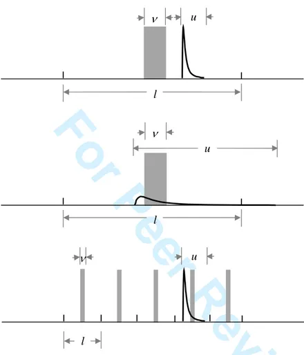
Figure 1 illustrates the sampling situation that forms the basis of this work. The upper figure represents a snapshot of the sampling of one stratum, as per a stratified punctual sampling scheme (discrete increments taken from the main flow at regular intervals of time of totalised mass). The extent of the sample increment is v, and that of the slug is u, expressed as a fraction of the lot. l is the extent of a sampling interval and is the reciprocal of the number of increments taken from the lot. For the sake of clarity, it was chosen here to show the situation where none of the slug falls inside the primary increment. This situation is highly probable as will be shown later, given the expected numbers of OTA-bearing slugs. Two types of strategies can clearly be adopted to intercept such slugs. The middle figure illustrates the case where the slug was smeared by mixing (dilution). Such a situation, which will occur to some extent during loading or unloading of a shipment, will increase the quality of sampling by decreasing spatial heterogeneity. Mixing should clearly be favoured in practical situations. The lowest figure shows a sampling strategy whereby increment mass is reduced, but sampling frequency is increased. Increasing sampling frequency, if possible, can also mitigate the 2 3 4 5 6 7 8 9 10 11 12 13 14 15 16 17 18 19 20 21 22 23 24 25 26 27 28 29 30 31 32 33 34 35 36 37 38 39 40 41 42 43 44 45 46 47 48 49 50 51 52 53 54 55 56 57 58

For Peer Review Only

OTA sampling problem. There is however a limit to the sampling frequency and increment mass that can be achieved in practice while obeying the accepted rules of correct sampling. Quantitative results pertaining to both these sampling mitigation options are presented in this paper.

From this difficult situation, analysis of sampling campaign data using conventional sampling variance analysis is a serious issue. In the process industries, time-wise correlation of analytes is to be expected and is almost always found to be present. When this correlation is characterised using a variogram, sampling variance calculations can determine the true primary stage sampling variance. However, if the analyte variations are random (no time-wise correlation), such calculations cannot be carried out. In such a case a statistical method such as developed herein must be used.

In this paper, we seek to explore the effect of changing increment mass and sampling frequency on the variance of sampling at various levels of OTA

contamination. We look at the situation from a mathematical perspective first, and present analytical results for special situations. This gives a first quantitative measure of the situation described in Figure 1. Because conventional sampling variance analysis cannot be used with randomly occurring contamination, we then review the complexity of OTA sampling by Monte Carlo simulation using actual design examples. The calculations were carried out in code written by the authors. We build our analysis on the whole sampling distribution of OTA in primary composite samples. Key cross-stream sampling parameters, namely increment mass and sampling frequency are varied in this analysis at a series of contamination levels. The results demonstrate the intrinsic limitations of conventional cross-stream sampling for OTA sampling.

Using the full distribution of the primary composite sample concentration, the results can be presented as operational characteristic (OC) curves.

2 3 4 5 6 7 8 9 10 11 12 13 14 15 16 17 18 19 20 21 22 23 24 25 26 27 28 29 30 31 32 33 34 35 36 37 38 39 40 41 42 43 44 45 46 47 48 49 50 51 52 53 54 55 56 57 58 59

For Peer Review Only

Preliminary problem analysis

The theoretical framework and key analytical results that are used in this paper have already been presented elsewhere by the authors (Lyman and Bourgeois, 2011) in the case of fixed length and fixed concentration of OTA-bearing slugs. A number of important results that correspond to this situation have been established, and the reasoning and analytical results that follow are directly based on the aforementioned publication.

The lot is divided into n strata of extent l, and is normalised to unity, such that 1

n l× = . The sample increments, of extent v, are placed centrally within each stratum. Hence a total of n sample increments are taken in the process. The slugs of

contaminated material are of a constant extent u, and m such slugs occur randomly in the lot; the slugs may overlap. Illustrations of these definitions are found in Figure 1.

We define three distinct MT concentrations (ng g-1):

• CL, the MT concentration of the lot of extent L (L = ). 1

• C0, the MT concentration in a slug, of extent u.

• CS, the MT concentration of the primary composite sample, of extent n×v.

The average number of slugs m in the lot is given by:

{ }

₃ 0 E E 6 L L bulk M C m Cπd _ρ =       (2)

where M is the mass of a lot and d is the diameter of the slug. The bulk density for _L

wheat is approximately ρbulk = 800 kg m-3 (Canadian Grain Commission, 2012b). If both

2 3 4 5 6 7 8 9 10 11 12 13 14 15 16 17 18 19 20 21 22 23 24 25 26 27 28 29 30 31 32 33 34 35 36 37 38 39 40 41 42 43 44 45 46 47 48 49 50 51 52 53 54 55 56 57 58

For Peer Review Only

the diameter d and concentration C0 of slugs are constant, then the expectations E{}

vanish from equation (2).

The statistical analysis of the problem can be viewed as a Bernoulli process, which consists of ‘throwing’ slugs independently into the structure of the n equally spaced sampling increments. Slugs can therefore overlap. Each slug has a probability

{ }

E u v q l + = (3)

of hitting an increment. With E{m} slugs in the lot, the probability of having j slugs hit the sample increments will be binomial with

{ }

{

}

₍

_{{ }}

E

{ }

!

₎

(

)

E{ } Pr E , 1 E ! ! m j j m j m q q q m j j − = − − (4)

The expected value and variance of the number of hits j are

{ }

{

}

{ }

{ }

{

}

{ }

(

)

E E , E var E , E 1 j m q m q j m q m q q = × = × × − (5)

We may first consider the probability of detecting slugs during sampling, as a function of the number of slugs per unit sampling length and the extents u and v of slugs and sample increments respectively. This probability is

{ }

{

}

(

)

E{ } E

{ }

E{ } 1 Pr 0 E , 1 1 1 1 m m u v j m q q l +   − = = − − = − −_{ }   (6)

Let us consider a base case scenario where the lot M =_L 2000 t and the mass

flow is m&_{L= 1000 tph. Such a lot size corresponds to a small wheat export cargo or to} 2 3 4 5 6 7 8 9 10 11 12 13 14 15 16 17 18 19 20 21 22 23 24 25 26 27 28 29 30 31 32 33 34 35 36 37 38 39 40 41 42 43 44 45 46 47 48 49 50 51 52 53 54 55 56 57 58 59

For Peer Review Only

the sampling unit used to sample the larger export cargos, whose size can reach about 50000 t. Increments are taken every 40 seconds using a cross-stream sampler with aperture wc = 19mm and linear velocity vc = 0.5 m/s. The increment mass mI is given by

1000 0.019 10.6 kg 3.6 3.6 0.5 c L I c w m m v = & × = × = (7)

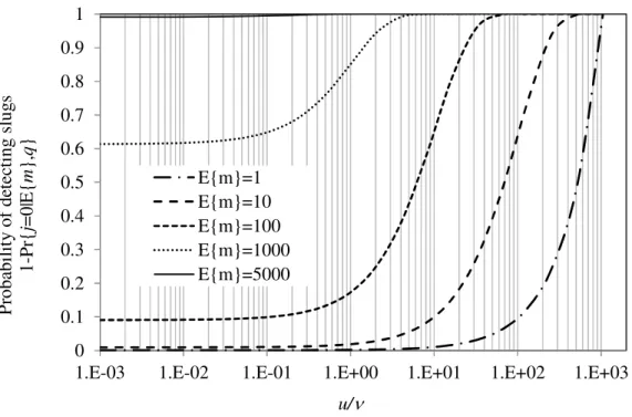
The 180 increments that are taken from the lot make up a primary composite sample mass of 1900 kg. With the extent of the lot normalized to unity, the stratum length l = 0.0056 and the increment length v=5.28 10× −6. The sampling ratio is

1:1053 v

n L

× = . Figure 2 shows the probability of a slug falling into the composite

sample as a function of the total number m of slugs per unit sampling length and the ratio of slug to sample increment mass u/v.

Let us assume that E{C0,undiluted} = 4000 ng g-1 and E{dundiluted} = 0.3 m for

undiluted slugs at the point of origin of the grain, and that they get diluted by a factor of 16 by the time the grain reaches its final point of destination. Diluted slugs will then

have E{C0} = E{C0,undiluted}/dilution = 250 ng g-1 and E

{ }

d =3dilution E×

{

d_undiluted

}

= 0.73 m (justification for these assumed values will be given later). If the average lot MT concentration CL = 2 ng g-1, the average number of slugs per 2000 t is E{m}=100.

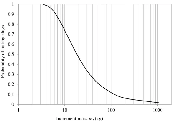
With 10.6 kg increments, the probability of hitting one or more slugs is 78.7%. In other words, primary composite samples will bear no MT 21.3% of the time, although the consignment carries 2 ng g-1 OTA on average. Assuming we double the sampling frequency and half the increment mass, mI = 5.3 kg, such that the primary composite

sample mass stays at 1900 kg, the probability of hitting one or more slugs will now increase to 95.1%, leaving the MT undetected 4.9% of the time. Figure 3 shows the relationship between the probability of hitting slugs and the increment mass for the base 2 3 4 5 6 7 8 9 10 11 12 13 14 15 16 17 18 19 20 21 22 23 24 25 26 27 28 29 30 31 32 33 34 35 36 37 38 39 40 41 42 43 44 45 46 47 48 49 50 51 52 53 54 55 56 57 58

For Peer Review Only

case scenario. It is emphasised that the higher the probability of hitting slugs, the lower the sampling variance, as shown mathematically by Lyman et al. (2009).

This simple analysis permits stating the obvious about sampling strategies for slug detection and reducing sampling variance. Indeed, it clearly shows, for the same primary composite sample mass that it is always sensible to increase the ratio u/v, either by increasing sampling frequency (i.e. decrease v) and decreasing increment mass mI.

The ratio u/v could also be increased by increasing dilution (i.e. increase the slug extent u), a fact that was noted by Biselli et al. (2008) who discussed the benefits of blending OTA slugs for reducing sampling variance due to spatial heterogeneity. We also note from Figure 2 that the lesser the number of slugs, the more critical the choice of

sampling conditions. Of course, increasing the primary composite sample mass will also reduce the sampling variance (Whitaker and Dickens, 1979). However, throughout this paper, it was decided to keep the increment sample mass constant as per the base scenario, which meets common practice. Excessive masses of primary increments present substantial problems in further mass division.

What Figure 2 also shows is that it appears extremely difficult, if not impossible, to justify stratified punctual sampling parameters without prior knowledge of the

number and size of slugs in the lot. This statement should provide a very strong incentive for in-situ characterisation campaigns of shipments and other consignments, for which data are currently lacking. It also raises questions about the adequacy of cross-stream sampling for detection of MTs in large grain consignments.

Ensuring that stratified cross-stream sampling parameters are such that sample increments have a significant probability of hitting slugs is not sufficient however to characterise a lot. Indeed, what is missing in the previous analysis is the prediction of MT concentration in the primary composite sample, from which one may decide to 2 3 4 5 6 7 8 9 10 11 12 13 14 15 16 17 18 19 20 21 22 23 24 25 26 27 28 29 30 31 32 33 34 35 36 37 38 39 40 41 42 43 44 45 46 47 48 49 50 51 52 53 54 55 56 57 58 59

For Peer Review Only

accept or reject a lot by comparison with some quality criterion. MT concentration in the primary composite sample should be characterised, at the very least, by estimates of mean and variance values. Lyman and Bourgeois (2011) have derived analytical expressions for both these statistical parameters in the case of slugs with fixed length u and uniform concentration C0. The analytical expressions can be extended to the case

where slugs have variable MT concentration by replacing C0 with E C

{ }

₀ in the

expression for the expected concentration and 2 0

C by E C

{ }

₀2 in the expression for the variance. The predictive equations are:

{ }

{ }

0 E C_S E C mu nl = (8) for u < v :

{ }

{ }

{ }

2 ₂ 0 2 0 E 1 1 2 1 E E 3 S C S C _{uv u} n C C nm u v v σ ₌   − ₊ ₋   ₊         (9) for u ≥ v :

{ }

{ }

{ }

2 ₂ 0 2 0 E 1 1 2 1 E E 3 S C S C _{uv v} n C C nm u v u σ ₌   − ₊ ₋  _{ +}        (10)

Equations (8) through (10) have significant utility to the analysis of this

sampling problem from analysis of variance, and the reader is invited to consult Lyman et al. (2009) to best appreciate the predictive strength of these analytical results.

However, they fail to deliver a complete picture of the distribution of MT in primary composite samples. Only knowledge of the whole MT concentration distribution in 2 3 4 5 6 7 8 9 10 11 12 13 14 15 16 17 18 19 20 21 22 23 24 25 26 27 28 29 30 31 32 33 34 35 36 37 38 39 40 41 42 43 44 45 46 47 48 49 50 51 52 53 54 55 56 57 58

For Peer Review Only

primary composite samples would permit carrying out a risk analysis on lot contamination level.

Analytical derivation of this distribution is complex in simple cases, and

possibly unavailable for more complex situations. Hence it is chosen here to investigate the problem by simulation such that more in-depth understanding of the sampling problem can be gained.

Results and analysis

It is necessary to first define the bases for this sampling problem, such that conclusions derived in the paper have practical relevance. Definition of sound bases is in itself not a simple matter, as little is known about OTA hot spots in actual settings. Particular issues of significance concern both the intrinsic and distributional heterogeneity of hot spots, namely the distribution of OTA within a single hot spot (mean value, maximum value, distribution), the size of hot spots (diameter, size distribution) and the number of hot spots per unit volume of grain. Moreover, the degree of dilution of hot spots that occurs between the grower and the consumer is also largely unknown. Notwithstanding the lack of quantitative data available from field measurements, educated guesses, whose sensitivity can eventually be studied, can be made. Hot-spot or slug properties that are established hereafter are deemed sufficient to yield results from which applicable conclusions and trends can be derived. However, quantitative results reported in the paper cannot be generalised to field applications for which slug properties are not known.

Problem basis

The general consensus is that OTA is a toxic secondary metabolite produced by a number of fungal species that grow and feed on cereal and derived processed products 2 3 4 5 6 7 8 9 10 11 12 13 14 15 16 17 18 19 20 21 22 23 24 25 26 27 28 29 30 31 32 33 34 35 36 37 38 39 40 41 42 43 44 45 46 47 48 49 50 51 52 53 54 55 56 57 58 59

For Peer Review Only

during storage (Magnoli et al., 2006). The occurrence of OTA in cereal grains however is unpredictable to this day and depends on many factors (Duarte et al., 2010), of which moisture and temperature are the most significant with respect to fungi growth and MT production rate. Under favourable conditions of humidity and temperature, storage fungi extend continuously into fresh zones of substrate. Where it is occurring, fungal infestation may be pictured as a filamentous network that moves from one nutrient-exhausted kernel to the next, at a growth rate that depends on local conditions. Assuming an average growth rate of the order of 0.1 mm hr-1 over a 2-month storage period, the size of a single undisturbed hot spot will be of the order of 0.3 meter in diameter. The assumed growth rate is based on Czaban et al. (2006) who reported steady fungal colony diameter growth in the range 0.08 to 0.14 mm hr-1 for P.

verrucosum in the temperature range 15°C to 28°C over a 14-day period. Assuming a kernel bulk density of 800 kg m-3, one single hot spot may weigh around 10 kg. This value is of the same magnitude as typical increments collected in the field.

Up to the point of final destination, every handling step through which the grain passes will contribute to both spreading fungal spores and mixing (i.e. diluting)

mycotoxins. Here, we shall only keep track of the hot spots that were formed during initial storage, assuming this storage duration far exceeds that of subsequent storages and/or that subsequent storage conditions are in the temperature/humidity range that does not yield further growth of fungi. For argument’s sake, let us assume that the grain, which has been stored at a local storage elevator for a period of 2 months, is railed to the final shipping facility, from which it is loaded onto a barge. Let us further assume a 2-fold dilution factor per handling step, yielding an overall 24:1 or 16:1 dilution for 4 handling steps over the whole process. The initial hot spot will now spread over 0.20 m3 or 160 kg of grain, so that it is 0.73 m in diameter. Incidentally, this value was used 2 3 4 5 6 7 8 9 10 11 12 13 14 15 16 17 18 19 20 21 22 23 24 25 26 27 28 29 30 31 32 33 34 35 36 37 38 39 40 41 42 43 44 45 46 47 48 49 50 51 52 53 54 55 56 57 58

For Peer Review Only

earlier to investigate the probability for hitting slugs. Dilution is therefore a parameter that can potentially be varied to gain some appreciation of the effect of mixing on hot spot sampling, the final volume (or mass) of hot spots being directly proportional to the overall dilution ratio. Typical primary sampling will yield a primary composite sample of 1900 kg of grain per 2000 t using the previous conditions, giving u/v = 15. This situation would appear to be quite favourable according to Figure 1.

In any given simulation run, populating the 2000 t lot with slugs requires that we specify a number of undiluted slugs m, their MT concentration C i₀

( )

in ng g-1, the dimensionless size u(i) of each slug, i= K1, ,m and the dilution factor. The number of slugs m is a discrete random variable whose mean value E{m} is given by equation (2).

By analysis of laboratory measurements for contaminated wheat kernels, Lyman et al. (2009) established that the OTA concentration of contaminated kernels followed a lognormal distribution. This result was derived from analysis of 15 contaminated kernels carried out by the CGC (Lyman et al., 2009). These contaminated kernels had an average OTA concentration of 1620 ng g-1 and a maximum value of 5000 ng g-1 of OTA was measured on one kernel. Due to the small number of kernels analysed, it is plausible that the concentration can reach significantly higher values on some kernels. On this basis, this work assumes that undiluted slugs have an average concentration of 4000 ng g-1 and a maximum concentration of 20000 ng g-1. This is regarded as a rather conservative assumption in the absence of more information. Starting from

contaminated kernels with a lognormal distribution of OTA concentration, Lyman et al. (2009) proved that the OTA concentration of samples of a given size (10 kg) drawn from a wheat into which the contaminated kernels had been mixed would also follow a lognormal distribution. Consequently, the average MT concentration C i₀

( )

of undiluted grains is drawn from the lognormal distribution with µ = 7.94 and σ = 0.85, giving 2 3 4 5 6 7 8 9 10 11 12 13 14 15 16 17 18 19 20 21 22 23 24 25 26 27 28 29 30 31 32 33 34 35 36 37 38 39 40 41 42 43 44 45 46 47 48 49 50 51 52 53 54 55 56 57 58 59

For Peer Review Only

E{C0} = 4000 ng g-1 and C0 = 20000 ng g-1 at the 99% confidence level of the

lognormal distribution.

The mean dimensionless slug size is given by

{ }

{

0,

}

E E L undiluted C u m C = × (11) where

{

}

2 0, E exp 4000 2 undiluted C = _

µ

+

σ

_=   ng g

-1 _{applies to undiluted slugs.}

We choose to draw values of dimensionless slug extent u from a uniform distribution

{ }

{ }

E 3E U , 2 2 u u    

 , where the lower bound of the uniform distribution is arbitrarily

chosen equal to half the expected value E{u}. This gives a slug diameter d such that

{ }

{ }

1 3 1 3 6 E L E bulk M d u πρ   =     (12)

The final slug concentration is calculated by dividing E{C0, undiluted} by the

dilution factor.

In order to build additional randomness, we choose to draw the dilution factor

for individual slugs from a uniform distribution U 12, 20

[

]

, the mean dilution factor being 16 as explained earlier.

The numerical slug generation procedure iterates until a set of m’ slugs is found such that

( ) ( )

0 1 m L i C i u i C ′ = × ≅

∑

(13) 2 3 4 5 6 7 8 9 10 11 12 13 14 15 16 17 18 19 20 21 22 23 24 25 26 27 28 29 30 31 32 33 34 35 36 37 38 39 40 41 42 43 44 45 46 47 48 49 50 51 52 53 54 55 56 57 58

For Peer Review Only

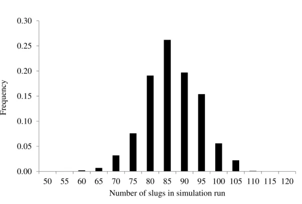
The convergence criterion for the slug generation algorithm is set to within a few percent of the target lot concentration. As an illustration of the randomness that is built into the simulations, Figure 4 gives an example of distribution of the number of slugs in 1000 simulations of a 2 ng g-1 lot. The mean number of slugs is 84.4 in this example and the actual mean lot contamination from the 1000 simulations is 2.18 ng g-1 (See Table 1).

The pivotal question that one may ask concerns the probability that such a lot might yield a primary composite sample whose MT content is greater than 5 ng g-1, recalling that the Commission Regulation (EC) No 1881/2006 sets the maximum acceptance limit for OTA concentration in raw cereal grain at 5 ng g-1. This value is used throughout this paper as the maximum admissible limit for the OTA or MT concentration of a lot. Conversely, what is the probability that a lot with average MT content greater than 5 ng g-1 might give a primary composite sample containing less than 5 ng g-1? This is best answered by calculating the distribution function of the composition of primary composite samples.

Distribution function of primary composite samples MT content

The distribution function is found by Monte Carlo simulation using code constructed by the authors, as mentioned earlier. The computational steps involved in arriving at a single result are as follows,

(1) choose the mean MT content of the lot

(2) find a slug MT concentration by sampling from the log-normal slug MT distribution

(3) find a slug extent by sampling from the uniform distribution defined above 2 3 4 5 6 7 8 9 10 11 12 13 14 15 16 17 18 19 20 21 22 23 24 25 26 27 28 29 30 31 32 33 34 35 36 37 38 39 40 41 42 43 44 45 46 47 48 49 50 51 52 53 54 55 56 57 58 59

For Peer Review Only

(4) find a dilution factor by sampling from the second uniform distribution defined above

(5) repeat steps 2 to 4 until equation (13) is adequately satisfied

(6) place the slugs into the one-dimensional lot following a uniform random distribution

(7) calculate the composition of the primary composite sample

(8) repeat steps 2 to 7 until 1000 realisations of the composition of the primary composite sample have been accumulated

(9) determine the mean and relative standard deviation ((standard deviation)/(mean concentration), expressed as a fraction not a percentage) of the composition of the primary composite samples over the 1000 realisations

(10) determine the empirical distribution function for the results from the 1000 realisations

The starting point is the calculation of the distribution of assays from simulation. Starting with the base case scenario, 1000 simulations were computed for mean lot MT contents above and below the acceptable limit ranging from, 10 ng g-1 to 2 ng g-1 respectively. Table 1 gives the mean MT content of the 1000 primary composite samples and the corresponding relative standard deviation for the 10 ng g-1 and 2 ng g-1 cases. The slug generation algorithm, which embeds a constrained level of randomness (variable slug extent, variable slug concentration, variable dilution of individual slugs), slightly overshoots the target lot concentration, with a mean lot concentration (1000 simulations) that is 3.7% higher on average than the target lot concentration. It can be verified however that there is no correlation between simulated mean lot MT content and sampling frequency; hence this slight overshoot is simply a consequence of the slug 2 3 4 5 6 7 8 9 10 11 12 13 14 15 16 17 18 19 20 21 22 23 24 25 26 27 28 29 30 31 32 33 34 35 36 37 38 39 40 41 42 43 44 45 46 47 48 49 50 51 52 53 54 55 56 57 58

For Peer Review Only

generation algorithm. Notwithstanding these slight differences, we shall refer to these cases as 2 ng g-1 and 10 ng g-1 in the rest of the paper.

As expected, Table 1 shows a causal relationship between sampling frequency or increment mass and the relative standard deviation of the mean concentration of the primary composite sample. What this means is that the uncertainty in the mean concentration of the lot increases monotonically with increasing increment mass. It is recalled that the mass of each of the 1000 primary composite samples is kept the same at 1900 kg for the 2000 t lot. Clearly, taking smaller increments at a higher rate yields a smaller sampling variance due to the spatial distribution of the slugs of MT. The values of Table 1 are the result of simulations, and the combinations of sampling frequency and increment mass of Table 1 are not all achievable in practice. An industrial cross-stream sampler width cannot be less than 10 mm (and should be three times the

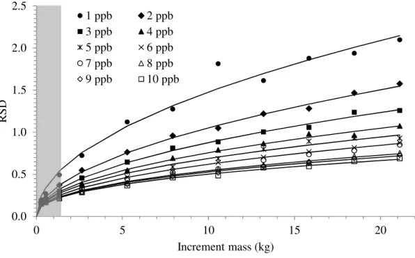
dimension of the largest particle), and its linear speed should not exceed 2 m s-1 (Cleary and Robinson, 2008) or even 0.6 m s-1 as prescribed by Gy (1982). Allowing the 10 mm aperture and the 2 m s-1 speed, the smallest increment mass achievable in practice would therefore be 1.4 kg in the base case scenario. For a 2000 t lot flowing at 1000 tph, a 1900 kg primary composite sample would have to be collected under these conditions at a sampling frequency of 5.3 s, which is close to the 5s / 1.3 kg combination from Table 1. Consequently, it would not be possible to obtain an RSD less than 0.37 and 0.21 for the 2 ng g-1 and 10 ng g-1 lots respectively. Above and beyond predictions from sampling theory, technological limitations of cross-stream sampling must also be built into the equation. Figure 5 shows the relationship between RSD and increment mass for a number of lot assays. The grey area shows the RSD values that cannot be accessed using a cross-stream sampler.

2 3 4 5 6 7 8 9 10 11 12 13 14 15 16 17 18 19 20 21 22 23 24 25 26 27 28 29 30 31 32 33 34 35 36 37 38 39 40 41 42 43 44 45 46 47 48 49 50 51 52 53 54 55 56 57 58 59

For Peer Review Only

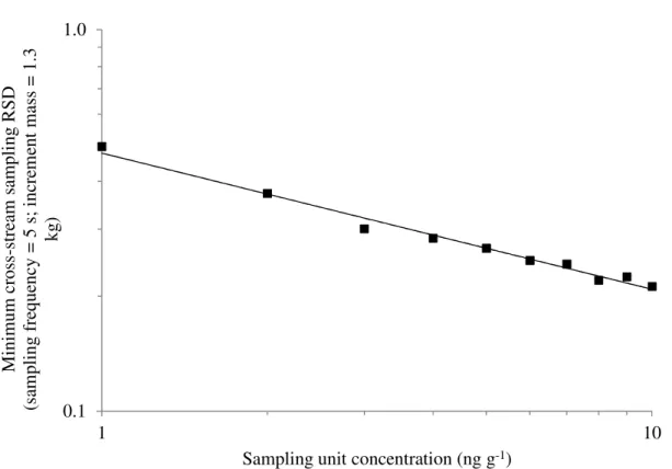
Figure 6 shows the minimum relative sampling standard deviation as a function of the lot concentration. Our simulation results indicate that the relationship is linear on

a log-log scale. A regression of the line yieldsRSD=0.4746×

(

MT

)

−0.357where MT is the lot concentration in ng g-1.

As shown above, analysis of sampling performance from mean and variance estimates yields insightful information that has direct practical application. However, it also gives an incomplete view of the problem in that skewness of the sampling

distribution is not evaluated. Indeed, not knowing what the MT distribution over the primary composite samples may be, it is not possible to state the probability of acceptance or rejection of a lot of a given quality without making some assumption about the underlying statistics. Making such assumptions about well mixed lots is not a problem as the distribution is almost surely normal. However, it becomes more and more hazardous as both intrinsic and distributional heterogeneities increase leading to possible gross departures from normality, which is precisely where the problem lies with sampling for mycotoxins such as OTA and other contaminants such as GMOs present in small concentrations.

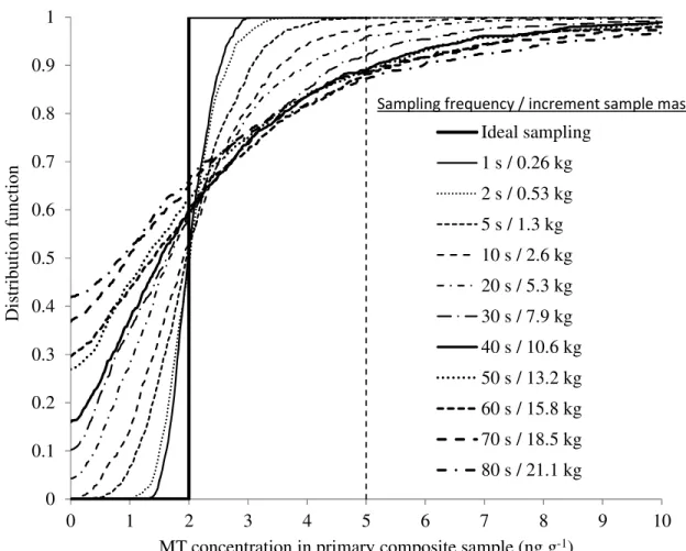
Distribution functions of MT concentrations for the 1000 primary composite samples are plotted in Figure 7 and Figure 8 for the 2 ng g-1 lots and 10 ng g-1 lots respectively.

Figures 7 and 8 show the dramatic effect of sampling frequency (alt. increment mass) on the probability distribution of the primary composite sample MT

concentration. Firstly, we recall from our previous calculation that any increment mass less than 1.4 kg is not achievable in practice with cross-stream cutters. Secondly, drawing a vertical line at the 5 ng g-1 acceptance limit shows that there is a finite probability of accepting a 10 ng g-1 lot, as well as a finite probability of rejecting a 2 ng 2 3 4 5 6 7 8 9 10 11 12 13 14 15 16 17 18 19 20 21 22 23 24 25 26 27 28 29 30 31 32 33 34 35 36 37 38 39 40 41 42 43 44 45 46 47 48 49 50 51 52 53 54 55 56 57 58

For Peer Review Only

g-1 lot. These probabilities, which can only be quantified with confidence from the full distribution of MT concentrations of primary composite samples, depend very strongly on increment mass due to the high level of DH created by MT-bearing slugs.

OC-curves

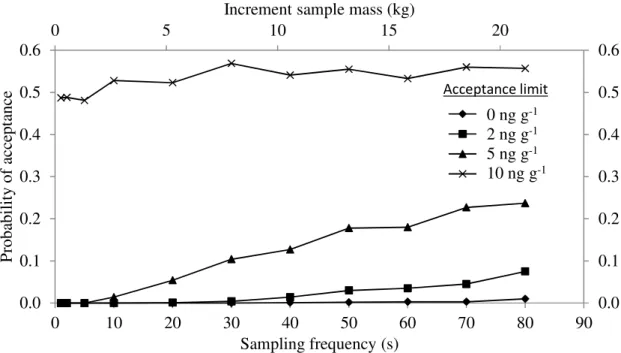
Figures 9 and 10 show the probability of acceptance and rejection of lots containing 10 ng g-1 and 2 ng g-1 MT respectively at 0, 2, 5 and 10 ng g-1 acceptance limits.

There is always some probability of acceptance of a 10 ng g-1 lot, even at the 0 ng g-1 acceptance limit. However, under the conditions of the simulations, it is less than 0.1% with the 40 s / 10.6 kg sampling scenario. At the 5 ng g-1 limit however, the probability of acceptance of a 10 ng g-1 lot is 13% with a 10.6 kg increment.

Conversely, there is always a finite probability of rejection of a 2 ng g-1 lot. Under the conditions of the simulations, Figure 10 shows that a 2 ng g-1 lot has a probability of rejection of 11.0% at the 5 ng g-1 acceptance limit with a 10.6 kg increment.

Perhaps the most complete way of representing and analyzing the probability of acceptance (alt. rejection) of a lot from sampling is achieved through the Operating Characteristic (OC) curve. Whitaker (2004) and Lyman et al. (2011) are useful

reference readings in relation to the application of OC curves for OTA sampling. This is a standard curve derived from statistical process control that links the probability of acceptance (type II error) of a lot to the mean property of a lot. Figure 11 shows the OC curves for a 5 ng g-1 acceptance limit for mean consignment contamination in the range 1 ng g-1 to 10 ng g-1. Each OC curve corresponds to one sampling frequency or

increment mass. Each point is the result of 1000 simulations. 2 3 4 5 6 7 8 9 10 11 12 13 14 15 16 17 18 19 20 21 22 23 24 25 26 27 28 29 30 31 32 33 34 35 36 37 38 39 40 41 42 43 44 45 46 47 48 49 50 51 52 53 54 55 56 57 58 59

For Peer Review Only

The OC curves all go through the origin, as there is no possibility of rejecting a lot that does not contain any mycotoxin. However, there is always a finite probability of rejecting or accepting a lot whose mean contamination level is less or higher than the acceptance limit.

The probability of rejecting an acceptable lot is referred to as the seller’s risk; a seller may see a perfectly acceptable lot rejected from after sampling. For example, with a sampling frequency of 40 s or 10.6 kg increments, a lot with MT concentration of 2 ng g-1 has an 11% chance of being rejected with a 1900 kg primary composite sample. Conversely, the probability of accepting a lot that assays more than the acceptable limit is referred to as the buyer’s risk; a buyer may accept an unacceptable lot after sampling. For example, with a sampling frequency of 40 s or 10.6 kg increment samples, a lot with MT concentration of 8 ng g-1 has a 28% chance of being accepted at the 5 ng g-1 level with a 1900 kg primary composite sample. It is emphasized that, without knowledge of the OC-curves, which are derived from knowledge of the full

concentration distribution of primary composite samples, there is no way for the seller or the buyer to quantify these probabilities.

Clearly, from a health viewpoint, the buyer’s risk is critical. If one decides that the buyer’s risk of accepting a 10 ng g-1 lot should be 5% or less, the OC curves from Figure 11 indicate that the sampling frequency should be no greater than 20s, which corresponds to an increment sampling mass of 5.3 kg when selecting a 1900 kg primary composite sample. In other words, over the 2000 t lot flowing at 1000 tph, 360

increments with a mass of 5.3 kg will give a 5% chance or less of accepting a lot when the primary composite sample contains 10 ng g-1 or less.

The value of knowing the complete distribution of primary composite sample assays is great. For every sampling condition, both seller’s and buyer’s risk are known 2 3 4 5 6 7 8 9 10 11 12 13 14 15 16 17 18 19 20 21 22 23 24 25 26 27 28 29 30 31 32 33 34 35 36 37 38 39 40 41 42 43 44 45 46 47 48 49 50 51 52 53 54 55 56 57 58

For Peer Review Only

and sampling strategy stands on firm ground. It is noted however that this analysis does not account for sample preparation and analysis uncertainties, which have relative standard deviations of about 5% and 10% respectively. Hence, Figure 11 is actually showing the minimal OC curves.

Discussion

The results that are built into the OC curves and other results above originate from matching the quality of the sampling scheme to the DH due to the slugs when selecting a 1900 kg primary composite sample from the 2000 t lot. Figure 12 shows frequency distributions of contamination in 1000 primary composite samples from a 2 ng g-1 lot for 3 of the sampling frequencies discussed above.

In addition to the skewness of these distributions, one striking feature of Figure 12 is the level of contrast between the distributions of primary composite samples and the increment mass. At the 1s and 10s sampling frequencies, Figure 12 shows that the probability that a primary composite sample will contain material from a slug is 100%. With the 10.6 kg increment, the probability that a primary composite sample will contain material from a slug is 83.7%, which means that primary composite samples will not contain any OTA 16.3 % of the time. It is noted that the theoretical probability from Equation (5) is 21.3%, the difference originating from the randomness built into the simulation. These numbers are a direct consequence of the DH created by the slugs, which yields a probability of hitting a slug that decreases very rapidly with increasing increment mass. The variation of any one slug being sampled by the primary sample, as calculated with 1000 simulations, was found to follow a log-log relationship, which is plotted in Figure 13.

Clearly, these probabilities highlight the failings of cross-stream sampling in coping with the DH of MT slugs inside the 2000 t lot.

2 3 4 5 6 7 8 9 10 11 12 13 14 15 16 17 18 19 20 21 22 23 24 25 26 27 28 29 30 31 32 33 34 35 36 37 38 39 40 41 42 43 44 45 46 47 48 49 50 51 52 53 54 55 56 57 58 59

For Peer Review Only

Although it has been demonstrated here that the limitations of cross-stream sampling for OTA analysis are intrinsic to the technique itself, it must be acknowledged that its failings can be partly offset by the size of the shipment. To illustrate this point, the distribution of primary composite sample concentration from Figure 12c, which corresponds to the 40 s frequency / 10.6 kg increment sampling scheme was resampled such that the aggregated mass would match shipment sizes ranging from 2000 to 300000 t, bearing in mind that export cargos will not exceed 50000 t in practice and are typically about 10000 t. Figure 14 shows the resulting distributions of MT concentration in a shipment as a function of shipment size. It is emphasised that sampling error is only due to primary sampling, and subsampling, preparatory and analytical errors will have to be added to these values. Typical values for these errors can be found in Vargas at al. (2004).

Under the assumptions used in this paper, with the 40 s frequency / 10.6 kg increment sampling scheme, Figure 14 shows that the rate of false positives (shipment assay > 5 ng g-1 limit) will be nearly zero when the shipment size exceeds 10000 t for a shipment that assays 2 ng g-1. Under favorable conditions, there may indeed be a combination of cross-cutting sampling conditions (sampling unit mass, primary

composite sample mass and increment mass) which, for a given shipment mass and MT assay, will yield an acceptable rate of false positives.

Conclusions

The paper applies a base case scenario that is deemed relevant to field practice, despite the lack of data about OTA occurrence in commercial shipments and storages. The base case uses industrial sampling guidelines at 1000 tph loading rate, and applies a justified level of randomness on both intrinsic and distributional heterogeneity of MT slugs, as 2 3 4 5 6 7 8 9 10 11 12 13 14 15 16 17 18 19 20 21 22 23 24 25 26 27 28 29 30 31 32 33 34 35 36 37 38 39 40 41 42 43 44 45 46 47 48 49 50 51 52 53 54 55 56 57 58

For Peer Review Only

well as a dilution factor related to mixing at grain handling stations. The work shows a causal relationship between sampling variance and sampling frequency, increment mass and dilution when selecting a 1900 kg primary composite sample from a 2000 t lot. Given the limited range of frequency and increment mass possible in industrial cross-stream sampling, this work shows that cross-cross-stream sampling exhibits a minimum sampling variance that varies with the mean shipment MT content.

The distribution of MT concentration for primary composite samples can be predicted by simulation. It shows the limitation of determination of sampling variance alone for determination of MTs in grain shipments, and the value of accessing the complete distribution statistics of primary composite samples for drawing reliable conclusions about shipment acceptability.

A number of conclusions can be derived from the results herein, given that the assumed slug characteristics are realistic.

It is fundamental to have access to the complete distribution statistics of primary composite samples in order to gain any real idea of the risk associated with a given sampling scheme, the missing link being the DH created by MT slugs. It would seem urgent to characterise the actual distribution of slug size and concentration in grain shipments or other large consignments. Such measurements are required to validate or invalidate current sampling protocols. Should convincing field data be available about the actual DH of slug properties, this work has also shown that simulation is clearly a useful companion tool for assessing the value of different sampling strategies.

Dilution (mixing) will definitely help sampling, as will increasing the sampling frequency. The level of mixing required to reach a desirable dilution will depend on the actual DH due to the slugs, which brings us back to the previous point.

2 3 4 5 6 7 8 9 10 11 12 13 14 15 16 17 18 19 20 21 22 23 24 25 26 27 28 29 30 31 32 33 34 35 36 37 38 39 40 41 42 43 44 45 46 47 48 49 50 51 52 53 54 55 56 57 58 59

For Peer Review Only

As we showed in Figure 6, cross-stream sampling exhibits an intrinsic limitation in that it is not possible to obtain a RSD value below 0.5 and 0.2 for 1 ng g-1 and 10 ng g-1 lots respectively, under the assumptions of this work. We showed that cross-stream sampling using a 40 s sampling frequency and 10.6 kg increments, which is often used in practice (Canadian Grain Commission Sampling Handbook, 2012), would have around a 10% chance of not containing any OTA with a 2 ng g-1 lot.

It was also shown that the larger the shipment size, the lower the rate of false positives for a given sampling scheme, so that cross-stream sampling may provide acceptable sampling performance in favourable situations.

It may be that conditions leading to the contamination of grain shipments by MTs are so variable, that no single sampling scheme involving cross-stream samplers can be endorsed. Cross-stream samplers appear to be intrinsically limited in their ability to provide sampling schemes suited to high DH lots. Sampling such material puts the grain sampling problem high on the list of difficulty. Perhaps the real solution is to find a means of sampling that eliminates the limitations exposed by this work.

References

Biselli, S, Person, C, Syben, M. 2008. Investigation of the distribution of

deoxynivalenol and ochratoxin A contamination within a 26t truckload of wheat kernel. Mycotoxin Research. 24(2):98-104.

Canadian Grain Commission 2012a. Sampling Systems Handbook and Approval Guide: http://www.grainscanada.gc.ca/guides-guides/ssh-mse/sshm-mmse-eng.htm

Canadian Grain Commission 2012b. Test weights of Western Canadian Grain, http://www.grainscanada.gc.ca

Cleary, P.W, Robinson, G.K. 2008. Evaluation of cross-stream sample cutters using three-dimensional discrete element modeling. Chemical Engineering Science. 63:2980-2993. 2 3 4 5 6 7 8 9 10 11 12 13 14 15 16 17 18 19 20 21 22 23 24 25 26 27 28 29 30 31 32 33 34 35 36 37 38 39 40 41 42 43 44 45 46 47 48 49 50 51 52 53 54 55 56 57 58

For Peer Review Only

Czaban, J, Wróblewska, B, Stochmal, A, Janda, B. 2006. Growth of Penicillium

verrucosum and production of ochratoxin A on nonsterilized wheat grain Incubated at different temperatures and water content. Polish Journal of Microbiology. 55(4):321-331.

Duarte, S.C, Pena, A, Lino, C.M. 2010. A review on ochratoxin A occurrence and effects of processing of cereal and cereal derived food products. Food Microbiology. 27:187-198.

Gy P.M. 1982. Sampling of particulate material – theory and practice. Elsevier, Amsterdam

ISO 24333:2009, Cereals and cereal products: Sampling, ISO Geneva

Lyman, G.J, Bourgeois, F.S. 2011. Sampling with discrete contamination: One

dimensional lots with random uniform contamination distributions. Proceedings of the 5th World Conference on Sampling and Blending, Santiago, Chile. Lyman, G.J., Bourgeois, F.S., Tittlemier, S. 2011. Use of OC curves in quality control

with an example of sampling for mycotoxins. Proceedings of the 5th World Conference on Sampling and Blending, Santiago, Chile.

Lyman, G.J., Bourgeois, F.S., Gawalko, E., Roscoe, M. 2009. Estimation of the sampling constants for grains contaminated by mycotoxins and the impact on sampling precision. Proceedings of the 4th World Conference on Sampling and Blending, Cape Town, South Africa.

Magnoli, C., Hallak, C., Astoreca, A., Ponsone, L., Chiacchiera, S., Dalcero, A.M. 2006. Occurrence of ochratoxin A-producing fungi in commercial corn kernels in Argentina. Mycopathologia. 161:53-58.

Paoletti, C., Donatelli, M., Heissenberger, A., Grazioli, E., Larcher, S., Van den Eede. 2005. European Union Perspective – Sampling for testing of genetically

modified impurities. Proceedings of the 2nd World Conference on Sampling and Blending, Sunshine Coast, Australia.

Paoletti, C., et al. 2006. Kernel lot distribution assessment (KeLDA): a study on the distribution of GMO in large soybean shipments, European Food Research Technology, 224 129-139

The Commission of the European Communities, 2006. Commission Regulation (EC) No 401/2006, Official Journal of the European Union.

2 3 4 5 6 7 8 9 10 11 12 13 14 15 16 17 18 19 20 21 22 23 24 25 26 27 28 29 30 31 32 33 34 35 36 37 38 39 40 41 42 43 44 45 46 47 48 49 50 51 52 53 54 55 56 57 58 59

For Peer Review Only

Tittlemier, S.A., Varga, E., Scott, P.M., Krska, R. 2011. Sampling of cereals and cereal-based foods for the determination of ochratoxin A: an overview. Food Additives & Contaminants: Part A. 28(6):775-785.

Whitaker, T.B. 2004. Mycotoxins in Foods: Detection and Control. Eds: N. Magan and M. Olsen. Woodhead Publishing Limited, Cambridge. Sampling for Mycotoxins; p. 69-87.

Whitaker, T.B., Dickens, J.W. 1979. Variability associated with testing corn for aflatoxin. Journal of the American Oil Chemists' Society. 53(7):502-505.

Vargas, E., Whitaker, T., Santos, E., Slate, A., Lima, F., and França, R., 2004. Testing Green Coffee for Ochratoxin A, Part I: Estimation of Variance Components, Journal of AOAC International, 87(4):884-891.

2 3 4 5 6 7 8 9 10 11 12 13 14 15 16 17 18 19 20 21 22 23 24 25 26 27 28 29 30 31 32 33 34 35 36 37 38 39 40 41 42 43 44 45 46 47 48 49 50 51 52 53 54 55 56 57 58

For Peer Review Only

Table 1. Simulation results for lot contamination by discrete slugs as a function of sampling

frequency: 2000 t lot; 1000 t/h flow rate; mean assay: 10 ng g-1 ; 1900 kg primary composite sample; E{dundiluted}=0.3 m, E{C0}=4000 ppb; E{dilution factor} = 16 (1000 simulations).

Sampling frequency (s) Increment mass (kg) Number of increments 2 ng g-1 10 ng g-1 Mean lot MT conc. (ng g-1) RSD Mean lot MT conc. (ng g-1) RSD 1 0.26 7308 2.05 0.17 10.28 0.15 2 0.53 3585 2.06 0.22 10.26 0.17 5 1.3 1462 2.06 0.37 10.36 0.21 10 2.6 731 2.10 0.55 10.18 0.29 20 5.3 358 2.01 0.76 10.31 0.37 30 7.9 241 2.12 0.96 10.01 0.46 40 10.6 179 2.18 1.05 10.17 0.49 50 13.2 144 2.05 1.22 10.33 0.58 60 15.8 120 2.18 1.28 10.62 0.59 70 18.5 103 2.03 1.47 10.26 0.65 80 21.1 90 2.10 1.57 10.56 0.69 Average: 2.09 10.30 2 3 4 5 6 7 8 9 10 11 12 13 14 15 16 17 18 19 20 21 22 23 24 25 26 27 28 29 30 31 32 33 34 35 36 37 38 39 40 41 42 43 44 45 46 47 48 49 50 51 52 53 54 55 56 57 58 59

For Peer Review Only

Figure 1. Illustration of the OTA shipment sampling problem. u ν l l ν u u l ν 2 3 4 5 6 7 8 9 10 11 12 13 14 15 16 17 18 19 20 21 22 23 24 25 26 27 28 29 30 31 32 33 34 35 36 37 38 39 40 41 42 43 44 45 46 47 48 49 50 51 52 53 54 55 56 57 58

For Peer Review Only

Figure 2. Probability of slug detection as a function of expected number of slugs in the lot and slug to sample increment mass ratio.

0 0.1 0.2 0.3 0.4 0.5 0.6 0.7 0.8 0.9 1

1.E-03 1.E-02 1.E-01 1.E+00 1.E+01 1.E+02 1.E+03

P roba bi li ty of de te ct ing s lug s 1-P r{ j= 0| E { m } ,q } u/ν E{m}=1 E{m}=10 E{m}=100 E{m}=1000 E{m}=5000 2 3 4 5 6 7 8 9 10 11 12 13 14 15 16 17 18 19 20 21 22 23 24 25 26 27 28 29 30 31 32 33 34 35 36 37 38 39 40 41 42 43 44 45 46 47 48 49 50 51 52 53 54 55 56 57 58 59

For Peer Review Only

Figure 3. Probability of slug detection for the base case scenario. (Lot mass ML = 2000 tonnes;

Primary composite sample mass: 1900 kg). 0 0.1 0.2 0.3 0.4 0.5 0.6 0.7 0.8 0.9 1 1 10 100 1000 P roba bi li ty of hi tt ing s lug s Increment mass m_I(kg) 2 3 4 5 6 7 8 9 10 11 12 13 14 15 16 17 18 19 20 21 22 23 24 25 26 27 28 29 30 31 32 33 34 35 36 37 38 39 40 41 42 43 44 45 46 47 48 49 50 51 52 53 54 55 56 57 58

For Peer Review Only

Figure 4. Example of distribution of number of slugs in 1000 simulations of a 2 ng g-1 lot. 0.00 0.05 0.10 0.15 0.20 0.25 0.30 50 55 60 65 70 75 80 85 90 95 100 105 110 115 120 F re que nc y

Number of slugs in simulation run 2 3 4 5 6 7 8 9 10 11 12 13 14 15 16 17 18 19 20 21 22 23 24 25 26 27 28 29 30 31 32 33 34 35 36 37 38 39 40 41 42 43 44 45 46 47 48 49 50 51 52 53 54 55 56 57 58 59

For Peer Review Only

Figure 5. Simulated relationship between increment mass and RSD for a range of mean lot assay levels (Each point = 1000 simulations). Shaded area indicates infeasible sampling conditions. 0.0 0.5 1.0 1.5 2.0 2.5 0 5 10 15 20 R S D Increment mass (kg) 1 ppb 2 ppb 3 ppb 4 ppb 5 ppb 6 ppb 7 ppb 8 ppb 9 ppb 10 ppb 2 3 4 5 6 7 8 9 10 11 12 13 14 15 16 17 18 19 20 21 22 23 24 25 26 27 28 29 30 31 32 33 34 35 36 37 38 39 40 41 42 43 44 45 46 47 48 49 50 51 52 53 54 55 56 57 58

For Peer Review Only

Figure 6. Minimum sampling RSD achievable with a 1.3 kg increment sample as a function of lot concentration. 0.1 1.0 1 10 M ini m um c ros s-st re am s am pl ing R S D (s am pl ing f re que nc y = 5 s; i nc re m ent m as s = 1. 3 kg )

Sampling unit concentration (ng g-1₎

2 3 4 5 6 7 8 9 10 11 12 13 14 15 16 17 18 19 20 21 22 23 24 25 26 27 28 29 30 31 32 33 34 35 36 37 38 39 40 41 42 43 44 45 46 47 48 49 50 51 52 53 54 55 56 57 58 59

For Peer Review Only

Figure 7. Distribution of MT concentration of primary composite samples for a 10 ng g-1 lot as a function of sampling frequency / increment mass. Conditions used : 2000 t lot; 1000 t/h flow rate; 1900 kg primary composite sample; E{dundiluted} = 0.3 m, E{C0} = 4000 ng g-1;

E{dilution factor} = 16 (1000 simulations). 0 0.1 0.2 0.3 0.4 0.5 0.6 0.7 0.8 0.9 1 0 5 10 15 20 25 30 D is tr ibut ion F unc ti on

MT concentration in primary composite sample (ng g-1₎

Ideal sampling 1 s / 0.26 kg 2 s / 0.53 kg 5 s / 1.3 kg 10 s / 2.6 kg 20 s / 5.3 kg 30 s / 7.9 kg 40 s / 10.6 kg 50 s / 13.2 kg 60 s / 15.8 kg 70 s / 18.5 kg 80 s / 21.1 kg

Sampling frequency / increment sample mass

2 3 4 5 6 7 8 9 10 11 12 13 14 15 16 17 18 19 20 21 22 23 24 25 26 27 28 29 30 31 32 33 34 35 36 37 38 39 40 41 42 43 44 45 46 47 48 49 50 51 52 53 54 55 56 57 58

For Peer Review Only

Figure 8. Distribution of MT concentration of primary composite samples for a 2 ng g-1 lot as a function of sampling frequency / increment mass. Conditions used: 2000 t lot; 1000 t/h flow rate; 1900 kg primary composite sample; E{dundiluted} = 0.3 m, E{C0} = 4000 ng g-1;

E{dilution factor} = 16 (1000 simulations). 0 0.1 0.2 0.3 0.4 0.5 0.6 0.7 0.8 0.9 1 0 1 2 3 4 5 6 7 8 9 10 D is tr ibut ion func ti on

MT concentration in primary composite sample (ng g-1₎

Ideal sampling 1 s / 0.26 kg 2 s / 0.53 kg 5 s / 1.3 kg 10 s / 2.6 kg 20 s / 5.3 kg 30 s / 7.9 kg 40 s / 10.6 kg 50 s / 13.2 kg 60 s / 15.8 kg 70 s / 18.5 kg 80 s / 21.1 kg

Sampling frequency / increment sample mass

2 3 4 5 6 7 8 9 10 11 12 13 14 15 16 17 18 19 20 21 22 23 24 25 26 27 28 29 30 31 32 33 34 35 36 37 38 39 40 41 42 43 44 45 46 47 48 49 50 51 52 53 54 55 56 57 58 59

For Peer Review Only

Figure 9. Probability of acceptance of a 10 ng g-1 lot from primary composite sample assay distribution at different acceptance limits (1000 simulations).

0 5 10 15 20 0.0 0.1 0.2 0.3 0.4 0.5 0.6 0.0 0.1 0.2 0.3 0.4 0.5 0.6 0 10 20 30 40 50 60 70 80 90

Increment sample mass (kg)

P roba bi li ty of a cc ept anc e Sampling frequency (s) 0 ppb 2 ppb 5 ppb 10 ppb Acceptance limit 0 ng g-1 2 ng g-1 5 ng g-1 10 ng g-1 2 3 4 5 6 7 8 9 10 11 12 13 14 15 16 17 18 19 20 21 22 23 24 25 26 27 28 29 30 31 32 33 34 35 36 37 38 39 40 41 42 43 44 45 46 47 48 49 50 51 52 53 54 55 56 57 58

For Peer Review Only

Figure 10. Probability of rejection of a 2 ng g-1 lot from primary composite sample assay distribution at different acceptance limits (1000 simulations).

0 5 10 15 20 0.0 0.1 0.2 0.3 0.4 0.5 0.6 0.7 0.8 0.9 1.0 0.0 0.1 0.2 0.3 0.4 0.5 0.6 0.7 0.8 0.9 1.0 0 10 20 30 40 50 60 70 80 90

Increment sample mass (kg)

P roba bi li ty of r ej ec ti on Sampling frequency (s) 0 ppb 2 ppb 5 ppb 10 ppb 0 ng g-1 2 ng g-1 5 ng g-1 10 ng g-1 Acceptance limit 2 3 4 5 6 7 8 9 10 11 12 13 14 15 16 17 18 19 20 21 22 23 24 25 26 27 28 29 30 31 32 33 34 35 36 37 38 39 40 41 42 43 44 45 46 47 48 49 50 51 52 53 54 55 56 57 58 59