The Optimal Class Size for Object-Oriented Software: A Replicated Study

(1)

https://doi.org/10.4224/5765587

READ THESE TERMS AND CONDITIONS CAREFULLY BEFORE USING THIS WEBSITE.

https://nrc-publications.canada.ca/eng/copyright

Vous avez des questions? Nous pouvons vous aider. Pour communiquer directement avec un auteur, consultez la

première page de la revue dans laquelle son article a été publié afin de trouver ses coordonnées. Si vous n’arrivez pas à les repérer, communiquez avec nous à PublicationsArchive-ArchivesPublications@nrc-cnrc.gc.ca.

Questions? Contact the NRC Publications Archive team at

PublicationsArchive-ArchivesPublications@nrc-cnrc.gc.ca. If you wish to email the authors directly, please see the first page of the publication for their contact information.

NRC Publications Archive

Archives des publications du CNRC

For the publisher’s version, please access the DOI link below./ Pour consulter la version de l’éditeur, utilisez le lien DOI ci-dessous.

Access and use of this website and the material on it are subject to the Terms and Conditions set forth at

The Optimal Class Size for Object-Oriented Software: A Replicated

Study

El-Emam, Khaled; Benlarbi, S.; Goel, N.; Melo, W.; Lounis, H.; Rai, S.

https://publications-cnrc.canada.ca/fra/droits

L’accès à ce site Web et l’utilisation de son contenu sont assujettis aux conditions présentées dans le site LISEZ CES CONDITIONS ATTENTIVEMENT AVANT D’UTILISER CE SITE WEB.

NRC Publications Record / Notice d'Archives des publications de CNRC:

https://nrc-publications.canada.ca/eng/view/object/?id=e709a57a-b4b9-4e73-83e2-4adb489a9836 https://publications-cnrc.canada.ca/fra/voir/objet/?id=e709a57a-b4b9-4e73-83e2-4adb489a9836

(2)

National Research Council Canada Institute for Information Technology Conseil national de recherches Canada Institut de technologie de l'information

The Optimal Class Size for Object-Oriented

Software: A Replicated Study *

El-Emam, K., Benlarbi, S., Goel, N., Melo, W., Lounis, H., Rai, S.

March 2000

* published as NRC/ERB-1074. March 2000. 27 pages. NRC 43653.

National Research Council of Canada

Permission is granted to quote short excerpts and to reproduce figures and tables from this report, provided that the source of such material is fully acknowledged.

(3)

National Research Council Canada Institute for Information Technology Conseil national de recherches Canada Institut de Technologie de l’information

The Optimal Class Size for

Object-Oriented Software: A

Replicated Study

K. El Emam, S. Beniarbi, N. Goel, W. Melo,

H. Lounis, and S.N. Rai

March 2000

(4)

The Optimal Class Size for Object-Oriented Software:

A Replicated Study

Khaled El Emam1 Saida Benlarbi & Nishith Goel2

Walcelio Melo3 Hakim Lounis4 Shesh N. Rai5

Abstract

A growing body of literature suggests that there is an optimal size for software components. This means that components that are too small or too big will have a higher defect content (i.e., there is a U-shaped curve relating defect content to size). The U-shaped curve has become known as the “Goldilocks Conjecture”. Recently, a cognitive theory has been proposed to explain this phenomenon, and it has been expanded to characterize object-oriented software. This conjecture has wide implications for software engineering practice. It suggests (1) that designers should deliberately strive to design classes that are of the optimal size, (2) that program decomposition is harmful, and (3) that there exists a maximum (threshold) class size that should not be exceeded to ensure fewer faults in the software. The purpose of the current paper is to evaluate this conjecture for object-oriented systems. We first demonstrate that the claims of an optimal component/class size (1 above) and of smaller components/classes having a greater defect content (2 above) are due to a mathematical artifact in the analyses performed previously. We then empirically test the threshold effect claims of this conjecture (3 above). To our knowledge, the empirical test of size threshold effects for object-oriented systems has not been performed thus far. We perform an initial study with an industrial C++ system, and replicated it twice on another C++ system and on a commercial Java application. Our results provide unambiguous evidence that there is no threshold effect of class size. We obtained the same result for three systems using 4 different size measures. These findings suggest that there is a simple continuous relationship between class size and faults, and that optimal class size, smaller classes are better, and threshold effects conjectures have no sound theoretical nor empirical basis.

1 Introduction

An emerging theory in the software engineering literature suggests that there is an optimal size for software components. This means that components that are of approximately this size are least likely to contain a fault, or will contain relatively less faults than other components further away from the optimal size.6 This optimal size has been stated to be, for example, 225 LOC for Ada packages [55], 83 total Ada source statements [16], 400 LOC for Columbus-Assembler [39], 877 LOC for Jovial [24], 100-150 LOC for Pascal and Fortran code [35], 200-400 LOC irrespective of the language [29], 25-80 Executable LOC [2],

1

National Research Council of Canada, Institute for Information Technology, Building M-50, Montreal Road, Ottawa, Ontario, Canada K1A OR6. Khaled.El-Emam@iit.nrc.ca

2

Cistel Technology, 210 Colonnade Road, Suite 204, Nepean, Ontario, Canada K2E 7L5. {benlarbi, ngoel}@cistel.com

3

Oracle Brazil, SCN Qd. 2 Bl. A, Ed. Corporate, S. 604, 70712-900 Brasilia, DF, Brazil. wmelo@br.oracle.com

4_{CRIM, 550 Sherbrooke West, Suite 100, Montreal, Quebec, Canada H3A 1B9. hlounis@crim.ca}

5_{Dept. of Biostatistics & Epidemiology, St. Jude Children's Research Hospital, 332 N. Lauderdale St., Memphis, TN}

38105-2794, USA. shesh.rai@stjude.org

6

Note that the optimal size theory is stated in terms of components, which could be functions in the procedural paradigm and classes in the object-oriented paradigm. It is not stating that there is an optimal program size. Also note that the optimal size theory is stated and demonstrated in terms of fault minimzation, rather than other outcome measures such as maximizing maintenance productivity.

(5)

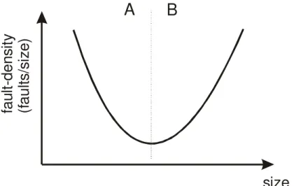
or 50-160 SLOC [2]. Card and Glass [12] note that military standards for module size range from 50 to 200 executable statements. Kan [34] plotted a curve of the relationship between LOC and fault-density for IBM’s AS/400, and concluded that there was indeed an optimal component size. This U-shaped curve is depicted in Figure 1 as it is often presented in the literature. It shows that fault-density is at a minimal value at a certain component size. Recently, Hatton [29] has articulated this theory forcefully and proposed a cognitive mechanism that would explain it. Fenton and Neil [20] term this theory the ‘Goldilocks Conjecture’.

size

fa

u

lt

-d

e

n

s

it

y

(f

a

u

lt

s

/s

iz

e

)

A

B

Figure 1: U-shaped curve relating fault-density to size that exemplifies the optimal size theory. The curve

can be broken up into two parts: A and B. The evidence that exists sometimes supports the whole curve, part A, or Part B.

Indeed, if the “Goldilocks Conjecture” is demonstrated to be an accurate description of reality, this would have wide implications on software engineering design. Designers should endeavor to decompose their systems such that most of their components are at or near optimal size. For instance, Withrow [55] has stated “software designers may decrease how error-prone their products are by decomposing problems in a way that leads to software modules that are neither too large nor too small.” and [16] “This study suggests that software engineers working with intermediate-size packages have an increased probability of producing software that is minimally defect-prone.” Kan [34] states “when an empirical optimum is derived by reasonable methods (for example, based on the previous release of the same product, or based on a similar product by the same development group), it can be used as a guideline for new module development.”

The evidence that does exist does not always support the U-shaped curve depicted above. Some studies demonstrate only part A in Figure 1. Others only support part B.

The first part of the Goldilocks Conjecture argues that smaller components have higher fault-proneness than larger components. There are number of empirical observations that demonstrate this. For example Basili and Perricone [1] observed that smaller Fortran components are likely to have greater fault-density, but did not identify an optimal component size. A similar observation was made by Davey et al. for C modules [17] and Selby and Basili [48] for routines written in a high-level language similar to PL/I used at the NASA GSFC. Shen et al. [49] analyzed data from three systems7 at IBM and found that fault density was higher for smaller components, but again did not identify a point where the fault-density would start to rise again for larger components. Moller and Paulish [39] found that components less than 70 LOC tended to have a higher fault-density than larger components. These results mean that reducing the size of components is detrimental to software quality. As noted by Fenton and Neil [20], this is counter to one

7

(6)

of the axioms of software engineering, namely program decomposition. In fact, this is one of the more explicit and controversial claims made by proponents of the optimal size theory [27][28][30].

Part B of Figure 1 illustrates another element of the Goldilocks Conjecture: that beyond a certain size, fault-proneness increases rapidly. This is in essence a threshold effect. For instance, Card and Glass [12] note that many programming texts suggest limiting component size to 50 or 60 SLOC. A study by O’Leary [40] of the relationship between size and faults in knowledge-based systems found no relationship between size and faults for small components, but a positive relationship for large components; again suggesting a threshold effect. A number of standards and organizations had defined upper limits on components size [7], for example, an upper limit of 200 source statements in MIL-STD-1679, 200 HOL executable statements in MIL-STD-1644A, 100 statements excluding annotation in RADC CP 0787796100E, 100 executable source lines in MILSTAR/ESD Spec, 200 source statements in MIL-STD-SDS, 200 source statements in MIL-STD-1679(A), and 200 HOL executable statements in FAA ER-130-005D. Bowen [7] proposed component size thresholds between 23-76 source statements based on his own analysis. After a lengthy critique of size thresholds, Dunn and Ullman [19] suggest two pages of source code listing as an indicator of an overly large component. Woodfield et al. [56] suggest a maximum threshold of 70 LOC.

The evidence for the Goldilocks Conjecture and its parts is not unequivocal, however. In fact, there exists some evidence that is completely contradictory. For instance, Card and Glass [12] re-analyze a data set using non-parametric techniques that on the surface suggested a higher fault-density for smaller components. The re-analysis found no relationship between size and fault-density. Fenton and Ohlsson [22] also found no obvious relationship between size and fault-density8 for a system at Ericsson.9

Some researchers have extended the argument for optimal component size to the object-oriented paradigm. For instance, Compton and Withrow [16] argue “We believe that the shape of the defect density curve [..] is fundamentally a reflection of optimal software decomposition, whether it was decomposed functionally or as objects.” Hatton [31] applies a memory model from cognitive psychology and concludes that there is a U-shaped relationship between fault-density and the class size of object-oriented software.

However, if smaller components are more likely to contain a fault than “medium-sized” components, this implies major problems for object-oriented programming10. The object-oriented strategies of limiting a class’ responsibility and reusing it in multiple contexts results in a profusion of small classes in object-oriented systems [54]. For instance, Chidamber and Kemerer [15] found in two systems studied11 that most classes tended to have a small number of methods (0-10), suggesting that most classes are relatively simple in their construction, providing specific abstraction and functionality. Another study of three systems performed at Bellcore12 found that half or more of the methods are fewer than four Smalltalk lines or two C++ statements, suggesting that the classes consist of small methods [54]. According to the Goldilocks Conjecture, this practice is detrimental to the quality of object-oriented applications.

Thresholds have been derived for the size of object-oriented classes. For instance, Lorenz and Kidd [36] recommend a maximum of 20 methods per class for non-UI classes13, 9 message sends per method, six LOC for Smalltalk methods, and 24 LOC for C++ methods. Rosenberg et al. [43] and French [23] present

8

This conclusion is based on the pooling of pre-release and post-release faults.

9_{Curiously, Card and Glass [12] initially examined a scatter plot of size vs. fault-density and concluded that it was misleading. They} subsequently grouped their data and based on that concluded that there was no relationship. Fenton and Ohlsson [22] on the other hand started off with the data grouped, and concluded that this way of analysis was misleading. They then examined a fault-density vs size scatter-plot, from which they concluded that there was no relationship.

10

An object-oriented component is defined as a class in this paper. 11

One system was in developed in C++, and the other in Smalltalk. 12

The study consisted of analyzing C++ and Smalltalk systems and interviewing the developers for two of them. For a C++ system, method size was measured as the number of executable statements, and for Smalltalk size was measured by uncommented nonblank lines of code.

13

(7)

a number of thresholds for class size. If the existence of thresholds can be supported through systematic empirical study, then that could greatly simplify quality management for object-oriented projects.14 However, none of these three studies demonstrated that indeed classes that exceed the thresholds are more fault-prone (i.e., the thresholds were not empirically validated).

From the above exposition it is clear that the implications of the optimal size theory on the design of object-oriented systems are significant. Even if only parts of the theory are found to be supportable, this would suggest important changes to current design or quality management practices. As noted above, however, the combination of evidence gives a confusing picture. This confusion makes acting on any of the above claims premature.

In this paper we present a theoretical and empirical evaluation of this conjecture for object-oriented applications. We first demonstrate that the claim of smaller components being more fault-prone than larger components to be a consequence of a mathematical artifact. We then test the threshold theory on three object-oriented applications. Our results provide clear evidence that there is no size threshold effect whatsoever. Hence, at least for object-oriented systems, the optimal size theory and its sub-parts are without support. We then state a simpler theory that matches our results.

In the next section we review the literature on the Goldilocks Conjecture and its parts. In Section 3 we describe in detail the research method that we used for testing the threshold effect theory, and our results are described in Section 4. We conclude the paper in Section 5 with an overall summary and the implications of our findings.

2 Background

The Goldilocks Conjecture stipulates that there exists an optimal component size,

S

. As component size increases or decreases away from

S

, the relative number of faults, or alternatively the probability of a fault, increases. This theory can be broken down into two parts that match A and B in Figure 1:

1. For any set of components with size

S

,

S

′

,

S

′′

, where

S

′′

<

S

′

<

S

, then

( )

S

D

( )

S

D

( )

S

D

′′

>

′

>

, where

D

( )

⋅

is the fault-density given the size

( )

⋅

.

2. For any set of components with size

S

,

S

′

,

S

′′

, where

S

′′

>

S

′

>

S

, then

( )

S

D

( )

S

D

( )

S

D

′′

>

′

>

, where

D

( )

⋅

is the fault-density given the size

( )

⋅

.

The evidence and arguments that support the whole of U-shaped curve phenomenon and the first part are similar, and therefore they are addressed jointly in the following subsection. We then consider the second part of the Goldilocks Conjecture.

2.1 The High Fault-Density of Small Components and The U-Shaped

Curve

A number of studies found a negative relationship between fault-density and some measure of size for

S

′

<

. For example, Basili and Perricone [1] analyzed testing and maintenance fault data for a Fortran project developed at the Software Engineering Laboratory. They found that smaller modules tended to have a larger fault density than larger modules. Size was measured in terms of executable lines of code. Davey et al. [17] found a similar pattern for C modules, Selby and Basili [48] observed the same phenomenon for routines written in a high-level language similar to PL/I, Shen et al. [49] reported the same pattern for three systems at IBM, and Moller and Paulish for systems at Siemens [39].

Other studies reported a U-shaped curve between fault-density and size. For example, Withrow [55] analyzed Ada software for command and control of a military communications system developed by a team of 17 professional programmers. Faults were logged during the test and integration phases. In total,

14

Thresholds provide a straight forward way for flagging classes that are high risk. Hence, they can be targeted for special defect detection activities, such as more extensive testing.

(8)

362 components were examined whereby a component is an Ada package. The results showed a U-shaped curve and gave a clear pattern of higher fault density for smaller components below an identified optimal component size. A subsequent study by Compton and Withrow [16] on an Ada system whereby they also collected faults during the first year post-release, found a similar pattern. Defect density tended to increase as component size decreased below the optimal size. Kan [34] plotted a curve of the relationship between LOC and fault-density for IBM’s AS/400 development, and concluded that there was indeed an optimal component size. When looking at components developed using the same programming language across releases, Moller and Paulish [39] identified the U-shaped curve for Columbus assmbler. Lind and Vairavan [35] identified the U-shaped curve for a real-time medical imaging system written mainly in Pascal and Fortran. They [35] explain the increase in fault-density after the minimal optimal value by stating that the complexity becomes too excessive for the programmers.

Size Measure N u m b e r o f F a u lts 0 4 8 12 16 20 24 Size Measure F a u lt D e n s ity (N u m b e r o f F a u lts /S iz e ) 0.00 0.01 0.02 0.03 0.04 0.05 0.06 0.07 0.08

(9)

Size Measure N u m b e r o f F a u lts 0 1 2 3 4 5 6 7 8 Size Measure F a u lt D e n s ity (N u m b e r o f F a u lts /S iz e ) 0.00 0.05 0.10 0.15 0.20 0.25 0.30 0.35 0.40

Figure 3: Relationship between component size and faults according to Hatton [29].

Fenton and Neil [20] provide an explanation for the above observations which they illustrate using a Bayesian Belief Network. They modeled a causal system of variables whereby a solution to a difficult problem was being designed. This leads to a larger design. Furthermore, their model specified that little testing effort was allocated. This means that few faults were detected during testing. Therefore, the larger the component, then the pre-release faults to size ratio will be small, and the smaller the component, the faults to size ratio will increase. This is the behavior observed in the studies above. A similar explanation can be derived for the case where testing was extensive and post-release faults. If testing was extensive then few faults will be found during operation. Therefore, the post-release faults to size ratio will be smaller for larger components, and larger for smaller components. However, this explanation fails somewhat in that the studies above were not focused solely on testing faults nor solely on post-release faults. In fact, a number of them incorporated both pre-release and post-release faults and the same effect was observed. The explanation is therefore not feasible since it is contradictory about the intensity of testing effort to explain the pre- and post-release phenomena. For example, the Selby and Basili [48] study included faults due to Trouble Reports, which are problems reported against working, released code. The studies of Basili and Perricone [1], Shen et al. [49], Moller and Paulish [39], and Compton and Withrow [16] included faults reported during the maintenance phase as well as testing. A number of further explanations for finding that smaller components have a larger fault content have been put forward:

• When just one part of a module is tested, other parts are to some degree also tested because of the connectivity of all the parts. Therefore, in a larger module, some parts may get “free testing” [55].

• Larger modules contain undiscovered faults because of inadequate test coverage [1][55], and therefore their fault density is low. Alternatively, faults in smaller modules are more apparent (e.g., easier to detect) [1].

• Interface faults tend to be evenly distributed among modules, and when converted to fault density, they produce larger values for small modules [1][55].

(10)

• In some data sets, the majority of components examined for analysis tended to be small, hence biasing the results [1].

• Larger components were coded with more care because of their size [1].

While the above explanations seem plausible, we will show that the observed phenomenon of smaller components having a higher fault-density is due to an arithmetic artifact. First, note that the above conclusions were drawn based exclusively on examination of the relationship between fault-density vs. size.

A plot of the basic relationship that Compton and Withrow [16] derived is shown in the top panel of Figure 2. If we represent exactly the same curve in terms of fault density, we get the curve in the lower panel. The top panel shows that as size increases, there will be more faults in a component. This makes intuitive sense. The bottom panel shows that smaller components tend to have a higher fault-density up to the optimal size (the lowest point in the curve), at which point fault-density is at a minima. However, by definition, if we model the relationship between any variable X and 1/X we will get a negative association as long as the relationship between size and faults is growing at most linearly. Rosenberg [42] has demonstrated this further with a Monte Carlo simulation, whereby he showed that the correlation between fault-density and size is always negative, irrespective of the distributions of size and faults, and their correlation. This is in fact a mathematical artifact of plotting a variable against its own reciprocal.

Similarly, the relationship between size15 and faults as derived by Hatton [29] is shown in the top panel in Figure 3. The bottom panel shows the relationship between fault-density and size. Again, the plotting of 1/X vs. X will, by definition, give you a negative association, whatever the variables may be.

Chayes [14] derives a formula for the correlation between 2 1

X

and

X

₂ when there is a zero correlation

between the two variables:

2 2 2 1 2 1 2 2 2 1

σ

µ

σ

µ

σ

µ

+

−

≈

r

Eqn. 1

where

µ

_i is the mean of variable

X

_i, and

σ

_i its standard deviation. It is clear that there will be a negative correlation, and possibly a large one (it depends on the variances and means of the ‘raw’ variables), even if the two ‘raw’ variables are not associated with each other. Therefore, drawing conclusions from a fault-density vs. size association is by no means an indication that there is an association at all, nor of it being a strong or weak one. On the other hand, as Takahashi and Kamayachi [51] demonstrate, if the relationship between faults and size is linear, then the association between fault-density and size will be almost zero, indicating that there is no impact of increased size when in fact there is a strong relationship between size and faults.16 Therefore, studying fault-density vs. size can actually mask and mislead us about the true relationship between size and fault content. By a medical analogy, we further show below how relationships can be easily distorted when you plot a compound measure with 1/X vs. X.

Consider a medical study whereby we want to look at the relationship between say exposure to a carcinogen and the incidence of cancer. For example, consider the data in the left panel in Figure 4. This shows the dose-response relationship between smoking intensity and mortality rates from lung cancer. It is clear that as the extent of smoking increases, the mortality rate increases. This is analogous to plotting the size versus the number of faults in our context. Now, if we plot the mortality per extent of smoking

15

The actual analysis used static path count. However, Hatton interprets the results to indicate a relationship between size and faults.

16

The unit of observation for the Takahashi and Kamayachi study was the program rather than the component. However, our interest here is with their analysis which demonstrates that not finding a relationship between fault-density and size may be simply due to a linear relationship between size and faults (not due to size have no effect on fault content).

(11)

versus the smoking intensity17, we get the right panel in Figure 4. This shows a clear U-shaped curve, suggesting, according to the practice outlined above, that there is an optimal smoking intensity of around 0.75 packs/day. It follows that low levels of smoking (around 0.25 packs/day) is associated with the highest risk of mortality from lung cancer!18

Packs/day M o rta li ty R a te p e r 1 0 0 ,0 0 0 p e rs o n -y e a rs 0 50 100 150 200 250

<0.5/day 0.5-1/day 1-2/day 2+/day

Packs/day M o rta li ty p e r S m o k in g I n te n s ity (P a c k s /d a y ) 0 50 100 150 200 250 <0.5/day (0.25) 0.5-1/day (0.75) 1-2/day (1.5) 2+/day (2)

Figure 4: Histogram showing the relationship between the intensity of smoking (packs/day) and the

mortality rate (the source of the data is [25]).

Another example is seen in Figure 5. This plots the mortality rate from lung cancer against exposure to uranium. The panel on the left shows the direct dose-response relationship, which clearly indicates the increasing mortality as exposure rises. By “normalizing” the mortality rate by the extent of exposure (as one would do by normalizing faults by size) we get exactly the opposite effect: that lower exposure is more harmful (see the panel on the right). Following the interpretation of this type of plot that is performed in the software engineering studies above, this would suggest that we should increase the exposure of people to uranium in order to reduce mortality.

17

Here, we took the mid-point of the smoking intensity variable, shown in parantheses in the histogram. 18

Note that in our curve we did not include the data for non-smokers. Including that and plotting mortality per smoking rate would give an infinite increase in lung cancer mortality for non-smokers.

(12)

WLM (mid-point) S M R 0 200 400 600 800 1000 1200 0 400 800 1200 1600 2000 2400 2800 WLM (mid-point) S R M /W L M 0.2 0.4 0.6 0.8 1.0 1.2 1.4 1.6 1.8 2.0 0 400 800 1200 1600 2000 2400 2800

Figure 5: Plots showing lung cancer risks amongst US uranium miners. The WLM is the working-level

month measure of cumulative exposure to uranium. The SMR19 is the standardized mortaility ratio. The data is obtained from [9].

As is seen from the above examples, the conclusions that are drawn defy common sense, and are clearly incorrect. This should illustrate that drawing conclusions from plots of fault-density against size is a practice that is not recommended.

The above exposition makes clear that the basic relationship is that as the size of the component grows, it will have more faults (or alternatively the likelihood of a fault increases). When one models a compound measure, such as fault density, against one of its components, meaningless conclusions can be easily drawn [42], and in fact, ones that are in exact opposition to the basic relationship.

2.2 Threshold Effect

Hatton [29] has proposed a cognitive explanation as to why a threshold effect would exist between size20 and faults. 21 The proposed theory is based on the human memory model, which consists of short-term and long-term memory. Hatton argues that Miller’s work [38] shows that humans can cope with around 7 +/- 2 pieces of information at a time in short-term memory, independent of information content. He then refers to [32] where they note that the contents of long-term memory are in a coded form and the recovery codes may get scrambled under some conditions. Short-term memory incorporates a rehearsal buffer that continuously refreshes itself. He suggests that anything that can fit into short-term memory is easier to understand and less fault-prone. Pieces that are too large overflow, involving use of the more error-prone recovery code mechanism used for long-term storage.

19

This is computed by comparing the actual number of deaths per year with the expected number of deaths per year of people of the same age in the general population.

20

Hatton uses the term “complexity” rather than size per se. However, he makes clear that he considers size to be a measure of complexity.

21

Hatton’s model also suggests that the size of objects should fill up short-term memory in order to utilize it efficiently, and that failure to do so also leads to increased fault-proneness. However, this aspect of his model is based on the types of analyses that we reviewed in Section 2.1, and showed that the conclusions from the observations are not sound. Therefore, we will not consider this aspect of Hatton’s model further.

(13)

Hatton’s theory states that a component of some size

S

fits entirely into short-term memory. If the component’s size exceeds

S

then short-term memory overflows. This makes the component less comprehensible because the recovery codes connecting comprehension with long-term memory break down. He then suggests a quadratic model that relates component size greater than

S

with the incidence of faults. In fact, Hatton’s explanation has some supporters in earlier software engineering work. For instance, Woodfield et al. [56] state “we hypothesize that there is a limit on the mental capacity of human beings. A person cannot manipulate information efficiently when its amount is much greater than that limit.”

Not all studies that looked at the relationship between size and faults found a threshold effect. For instance the studies by Basili and Perricone [1] and Davey et al. [17] mentioned above did note that the components for which they had data tended to be small, and therefore they could not observe the effect at large component sizes. One can consider the U-shaped curves identified by Withrow [55], Compton and Withrow [16], Moller and Paulish [39], Kan [34] as identifying a threshold effect. However, as shown in the previous section, plotting fault density against size does not make too much sense.

In a subsequent article, Hatton [31] extends this model to object-oriented development. He argues that the concept of encapsulation, central to object-oriented development, lets us think about an object in isolation. If the size of this object is small enough to fit into short-term memory, then it will be easier to understand and reason about. Objects that are too large and overflow the short-term memory tend to be more fault-prone.

There is ample evidence in the software engineering literature that the size of object-oriented classes is associated with fault-proneness. The relationship between size and faults is clearly visible in the study of [13], where the Spearman correlation was found to be 0.759 and statistically significant. Another study of image analysis programs written in C++ found a Spearman correlation of 0.53 between size in LOC and the number of errors found during testing [26], and was statistically significant at an alpha level of 0.05. Briand et al. [11] find statistically significant associations between 6 different size metrics and fault-proneness for C++ programs, with a change in odds ratio going as high as 4.952 for one of the size metrics. None of these studies, however, was concerned with size thresholds, and therefore did not test for them.

There has been interest in the industrial software engineering community with establishing thresholds for object-oriented measures. This was not driven by theoretical concerns, or a desire to test a theory, but rather with pragmatic ones. Thresholds provide a simple way for identifying problematic classes. If a class has a measurement value greater than the threshold then it is flagged for investigation.

Lorenz and Kidd present a catalogue of thresholds [36] based on their experiences with C++ and Smalltalk projects. Most notable for our purposes are the thresholds they propose for size measures. For example, they set a maximum threshold of 20 methods in a class, and three variables for non-user-interface classes. Rosenberg et al. [43] present a series of thresholds for various object-oriented metrics, for instance, they suggest a size threshold of 40 methods per class. French [23] presents a procedure for computing thresholds and applies it to object-oriented projects in Ada95 and C++. In none of the above three works was a systematic validation performed to demonstrate that classes that exceeded the threshold size were indeed more problematic than those that do not, e.g., that they were more likely to contain a fault.

2.3 Summary

To our knowledge, there have been no studies that compute and validate size thresholds for object-oriented applications. This means that the human memory model proposed by Hatton and the practical thresholds derived by other researchers have not been empirically validated. Therefore, the purpose of our study was to test the size threshold effect theory.

It should be noted that if the size threshold theory is substantiated, this could have important implications. Given that its premise is cognitive, it would be expected that similar thresholds will hold across professional programmers and designers, and hence have broad generalizability.

(14)

3 Research Method

3.1 Measurement

3.1.1 Size Measures

The size of a class can be measured in a number of different ways. Briand et al. [11] have summarized some common size measures for object-oriented systems, and these consist of:22

• Stmts: The number of declaration and executable statements in the methods of a class. This can

also be generalized to a simple SLOC count.

• NM (Number of Methods): The number of methods implemented in a class.

• NAI (Number of Attributes): The number of attributes in a class (excluding inherited ones). Includes

attributes of basic types such as strings and integers

As noted earlier, our initial study was performed on one C++ telecommunications system and replicated twice; once on another C++ system and once on a Java application. The studies were performed seperately over a period of 18 months, and were performed under different constraints. We were therefore not able to collect all of the size measures for all systems. For instance, for the Java system the objective was to focus on measures that could be collected at design time only, which excludes Stmts and SLOC. For each of the three systems, we present the subset of size measures that we collected.

3.1.2 Fault Measurement

In the context of building quantitative models of software faults, it has been argued that considering faults causing field failures is a more important question to address than faults found during testing [6]. In fact, it has been argued that it is the ultimate aim of quality modeling to identify post-release fault-proneness [21]. In at least one study it was found that pre-release fault-proneness is not a good surrogate measure for post-release fault-proness, the reason posited being that pre-release fault-proneness is a function of testing effort [22].

Therefore, faults counted for all the systems that we studied were due to field failures occuring during actual usage. For each class we characterized it as either faulty or not faulty. A faulty class had at least one fault detected during field operation. Distinct failures that are traced to the same fault are counted as a single fault.

3.2 Data Sources

Our study was performed on three object-oriented systems. It was initially done on C++ System 1, and then replicated on the subsequent two. These data sources are described below.

3.2.1 C++ System 1

This is a telecommunications system developed in C++, and has been in operation for approximately seven years. This system has been deployed around the world in multiple sites. In total six different developers had worked on its development and evolution. It consists of 83 different classes, all of which we analyzed.

Since the system has been evolving in functionality over the years, we selected a version for analysis where reliable fault data could be obtained.

Fault data was collected from the configuration management system. This documented the reason for each change made to the source code, and hence it was easy to identify which changes were due to faults. We focused on faults that were due to failures reported from the field. In total, 53 classes had one or more fault in them that was attributed to a field failure.

22

(15)

3.2.2 C++ System 2

Our data set comes from a telecommunications framework written in C++ [45]. The framework implements many core design patterns for concurrent communication software. The communication software tasks provided by this framework include event demultiplexing and event handler dispatching, signal handling, service initialization, interprocess communication, shared memory management, message routing, dynamic (re)configuration of distributed services, and concurrent execution and synchronization. The framework has been used in applications such as electronic medical imaging systems, configurable telecommunications systems, high-performance real-time CORBA, and web servers. Examples of its application include in the Motorola Iridium global personal communications system [47] and in network monitoring applications for telecommunications switches at Ericsson [46]. A total of 174 classes from the framework that were being reused in the development of commercial switching software constitute the system that we study. A total of 14 different programmers were involved in the development of this set of classes.23

For this product, we obtained data on the faults found in the library from actual field usage. Each fault was due to a unique field failure and represents a defect in the program that caused the failure. Failures were reported by the users of the framework. The developers of the framework documented the reasons for each delta in the version control system, and it was from this that we extracted information on whether a class was faulty. A total of 192 faults were detected in the framework at the time of writing. These faults occurred in 70 out of 174 classes.

3.2.3 Java System

This system is a commercial Java application. The application implements a word processor that can either be used stand-alone or embedded as a component within other larger applications. The word processor provides support for formatted text at the word, paragraph, and document levels, allows the definition of groupings of formatting elements as styles, supports RTF and HTML external file formats, allows spell checking of a range of words on demand, supports images embedded within documents or pointed to through links, and can interact with external databases.

This application was fielded and feedback was obtained from its users. This feedback included reports of failures and change requests for future enhancements. The application had a total of 69 classes. The size measures were collected from an especially developed static analysis tool. No Java inner classes were considered. For each class it was known how many field failures were associated to a fault in that class. In total, 27 classes had faults.

3.2.4 Size Measures

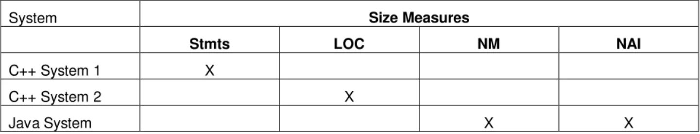
The size measures that were collected for each of the above three systems are summarized in Table 1.

System Size Measures

Stmts LOC NM NAI

C++ System 1 X

C++ System 2 X

Java System X X

Table 1: Table showing which size measures were collected for the different systems.

Across the three systems we covered different types of size measures. The measures STMTS and LOC are commonly only available from the source code. However, NM and NAI can be easily obtained from design documents. If we obtain consistent results across the systems and measures, then we can have greater confidence in the generalizability of our conclusions.

23

(16)

3.3 Analysis Method

The method that we use to perform our analysis is logistic regression. Logistic regression (LR) is used to construct models when the dependent variable is binary, as in our case. The general approach we use is to construct a LR model with no threshold, and a LR model with a threshold, and then compare the two models. This is the standard technique for evaluating LR models [33].

3.3.1 Logistic Regression

The general form of an LR model is:24

(

size

)

e

0 1

1

β β

π

₋ ₊

+

=

Eqn. 2

where

π

is the probability of a class having a fault. The

β

parameters are estimated through the (unconditional)25 maximization of a log-likelihood [33].

3.3.2 Diagnosing Collinearity

Collinearity is traditionally seen as being concerned with dependencies amongst independent variables. The models that we build in our study all involve only one independent variable, namely size. However, it is known that collinearities can exist between the independent variables and the intercept [50].

Previous studies have shown that outliers can induce collinearities in regression models [37][44]. But also, it is known that collinearities may mask influential observations [3]. This has lead some authors to recommend addressing potential collinearity problems as a first step in the analysis [3], and this is the sequence that we follow.

Belsley et al. [3] propose the condition number as a collinearity diagnostic for the case of ordinary least squares regression26 First, let

ß

ˆ

x be a vector of the parameter estimates, and

X

is a

n

×

(

k

+

1 )

matrix

of the

x

ij raw data, with

i

=

1 K

n

and

j

=

1 K

k

, where

n

is the number of observations and

k

is the number of independent variables. Here, the

X

_{matrix has a column of ones to account for the fact that}

the intercept is included in the models. The condition number can be obtained from the eigenvalues of the

X

T

X

_{matrix as follows:}

min max

µ

η =

Eqn. 3

where

µ

max

≥

L

≥

µ

min are the eigenvalues. Based on a number of experiments, Belsley et al. suggest that a condition number greater than 30 indicates mild to severe collinearity.

Belsley et al. emphasize that in the case where an intercept is included in the model, the independent variables should not be centered since this can mask the role of the constant in any near dependencies. Furthermore, the

X

_{matrix must be column equilibrated, that is, each column should be scaled for equal}

24

We also evaluated log and quadratic models in the logit. The conclusions were the same, and therefore we present the results for the linear model only.

25

Conditional logistic regression is used when matching of observations was performed during the study and each matched set is treated as a stratum in the analysis [8].

26

Actually, they propose a number of diagnostic tools. However, for the purposes of our analysis with only one independent variable we will consider the condition number only.

(17)

Euclidean length. Without this, the collinearity diagnostic produces arbitrary results. Column equilibration is achieved by scaling each column in

X

_,

j

X

_{, by its norm [4]:}

j

X

_.

This diagnostic has been extended specifically to the case of LR models [18][53] by capitalizing on the analogy between the independent variable cross-product matrix in least-squares regression to the information matrix in maximum likelihood estimation, and therefore it would certainly be parsimonious to use the latter.

The information matrix in the case of LR models is [33]:

( )

ß

X

V

X

I

ˆ

=

T

ˆ

_{Eqn. 4}

where

V

ˆ

is the diagonal matrix consisting of

π

ˆ

_ii

(

1 −

π

ˆ

_ii

)

where

π

ˆ

_ii is the probability estimate from the LR model for observation

i

. Note that the variance-covariance matrix of

ß

ˆ

_{is given by}

I

ˆ

−1

( )

ß

ˆ

_{. One can}

then compute the eigenvalues from the information matrix after column equilibrating and compute the condition number as in Eqn. 3. The general approach for non-least-squares models is described by Belsley [5]. In this case, the same interpretive guidelines as for the traditional condition number are used [53].

3.3.2.1 Hypothesis Testing

The next task in evaluating the LR model is to determine whether the regression parameter is different from zero, i.e., test

H

₀

:

β

₁

=

0

. This can be achieved by using the likelihood ratio

G

statistic [33]. One first determines the log-likelihood for the model with the constant term only, and denote this

l

0 for the ‘null’ model. Then the log-likelihood for the full model with the size parameter is determined, and denote this

l

_S. The

G

statistic is given by

2 (

l

_S

−

l

₀

)

which has a

χ

2 distribution with 1 degree of freedom.27 In previous studies with object-oriented measures another descriptive statistic has been used, namely an

2

R

statistic that is analogous to the multiple coefficient of determination in least-squares regression [10][11]. This is defined as 0 0 2

l

R

=

−

S

and may be interpreted as the proportion of uncertainty

explained by the model. We use a corrected version of this suggested by Hosmer and Lemeshow [33]. It should be recalled that this descriptive statistic will in general have low values compared to what one is accustomed to in a least-squares regression. In our study we will use the corrected

R

2 statistic as a loose indicator of the quality of the LR model.

3.3.2.2 Influence Analysis

Influence analysis is performed to identify influential observations (i.e., ones that have a large influence on the LR model). This can be achieved through deletion diagnostics. For a data set with

n

observations, estimated coefficients are recomputed

n

times, each time deleting one of the observations28 from the model fitting process. Pergibon has defined the

∆

β

diagnostic [41] to identify influential groups in logistic regression. The

∆

β

diagnostic is a standardized distance between the parameter estimates when a group of observations with the same

x

i values is included and when they are not included in the model.

27

Note that we are not concerned with testing whether the intercept is zero or not since we do not draw substantive conclusions from the intercept. If we were, we would use the log-likelihood for the null model which assigns a probability of 0.5 to each response.

28

(18)

We use the

∆

β

diagnostic in our study to identify influential groups of observations. For groups that are deemed influential we investigate this to determine if we can identify substantive reasons for them being overly influential. In all cases in our study where a large

∆

β

was detected, its removal, while affecting the estimated coefficients, did not alter our conclusions.

3.3.3 Model With A Threshold

A LR model with a threshold can be defined as [52]:

(

) (

)

(

β

τ

)

π

₋

₊

₋

+

=

_size

_I

_size

e

0 1

1

Eqn. 5 where:

( )







>

≤

=

+

0

1

0

0 z

if

z

if

z

I

Eqn. 6

and

τ

is the size threshold value. The difference between the no-threshold and threshold model is illustrated in Figure 6. For the threshold model the probability of a fault only starts to increase once the size is greater than the threshold value,

τ

.29

Size

π

(Size)

threshold

Figure 6: Relationship between size and the probability of a fault for the threshold and no-threshold

models.

To estimate the threshold value,

τ

, one can maximize the log-likelihood for the model in Eqn. 5. Ulm [52] presents an algorithm for performing this maximization.

Once a threshold is estimated, it should be evaluated. This is done by comparing the no-threshold model with the threshold model. Such a comparison is, as is typical, done using a likelihood ratio statistic (for example see [33]). The null hypothesis being tested is:

size

H

0

:

τ

≤

(1)

=

min

Eqn. 7

29

This type of model has been used in epidemiological studies, for example, to evaluate the threshold of dust concentrations in coal mines above which miners develop chronic bronchitic reactions [52]. In fact, the general approach can be applied to investigate any dose-response relationship that is postulated to have a threshold.

(19)

where

size

(1) is the smallest size value in the data set. If this null hypothesis is not rejected then it means that the threshold is equal to or below the minimal value. In the latter case, this is exactly like saying that the threshold model is the same as the no-threshold model. In the former case, the threshold model will be very similar to the no-threshold model since only a small proportion of the observations will have the minimal value. Hence one can conclude that there is no threshold. The alternative hypothesis is: ) 1 ( 1

:

size

H

τ

>

_{Eqn. 8}

which would indicate that a threshold effect exists.

The likelihood ratio statistic is computed as

−

2 (

ll

( ) ( )

H

0

−

ll

H

1

)

, where

ll

( )

⋅

is the log-likelihood for the given model. This can be compared to a

χ

2 distribution with 1 degree of freedom. We use an

α

level of 0.05. Ulm [52] has performed a Monte Carlo simulation to evaluate this test and subsequently recommended its use.

It should be noted that if

τ

ˆ

is equal or close to

size

(n) (the largest size value in the data set), this would mean that most of the observations in the data set would have a value of zero, making the estimated model parameters unstable. In such a case, we conclude that no threshold effect was found for this data set. Ideally, if a threshold exists then it should not be too close to the minimum or maximum values of size in the data set.

4 Results

4.1 Descriptive Statistics

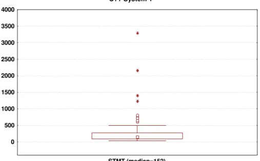
The plots in Figure 7, Figure 8, and Figure 9 show the dispersion and central tendency of size for the three systems. One thing that is noticeable from these plots is that C++ System 1 tends to have larger classes than C++ System 2. This is further emphasized when we consider that a statement is sometimes over multiple source lines. Hence, if we measure size for both systems on the same scale, it would become more obvious that System 1 is much larger.

Another point to note is that for each of the three systems there are extreme outliers. Although the outliers are not necessarily influential observations, they do provide support for being prudent and performing diagnostics for influential observations.

(20)

C++ System 1 0 500 1000 1500 2000 2500 3000 3500 4000 STMT (median=152)

Figure 7: Dispersion and central tendency of the size measure for C++ System 1.

C++ System 2 0 100 200 300 400 500 LOC (median=41.5)

(21)

Java System 0 10 20 30 40 50 60 70 80

NM (median=9) NAI (median=7)

Figure 9: Dispersion and central tendency of the size measure for the Java system.

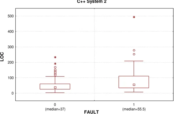
The box and whisker plots in Figure 10, Figure 11, Figure 12, and Figure 13 contrast the size of faulty and not-faulty classes. It is clear from these plots that faulty classes tend to be larger than not-faulty classes. In some cases, as in the Java system, more substantially so.

C++ System 1 FAULT S T M T 0 500 1000 1500 2000 2500 3000 3500 0 (median=129.5) 1 (median=168)

(22)

C++ System 2 FAULT L O C 0 100 200 300 400 500 0 (median=37) 1 (median=55.5)

Figure 11: Dispersion and central tendency for faulty (1) and non-faulty (0) classes in C++ System 2.

Java System FAULT N M 0 10 20 30 40 50 60 70 80 0 (median=7) 1 (median=13)

Figure 12: Dispersion and central tendency for faulty (1) and non-faulty (0) classes in the Java System

(23)

Java System FAULT N A I 0 10 20 30 40 0 (median=1) 1 (median=9)

Figure 13: Dispersion and central tendency for faulty and non-fault classes in the Java System and the

NAI size measure

4.2 Testing For Threshold Effects

The results of testing for threshold effects are presented in Table 2, Table 3, Table 4, and Table 5 for the four size measures across the three systems. The tables show the parameters for the no-threshold model (Eqn. 2), the threshold model (Eqn. 5), and their comparison. The bottom row shows the estimated threshold value, the chi-square value from comparing the two models, and its p-value. Even though a threshold value was estimated, the threshold model must have a statistically significant difference from the no-threshold model in order to reject the null hypothesis.

A number of general trends can be observed from these tables. First, that for all the threshold and no-threshold models, size has a positive parameter and is always statistically significant. However, this is not surprising and is consistent with previous results. Second, the condition number is always below 30, indicating that there are no collinearity problems in any of the models. Third, The R2 measures tend to run low. However, as noted earlier for logistic regression this is common, and also one should not expect that a simple model with only size will provide substantial explanatory power (for our purposes of testing the threshold hypothesis, however, this size only model is all that is required). Finally, that in none of the comparisons performed was there a difference between the threshold and no-threshold models. This indicates that there are no threshold effects.

(24)

STMT

No Threshold Model R2

LR

η

β1 Coefficient (s.e.) p-value

0.040 2.446 0.001915 (0.001261) 0.036 Threshold Model R2 LR

η

0.061 1.011 0.1061

(0.3743)

0.01

Comparison of Models

Estimated Threshold Value Chi-Square p-value

671 2.256 0.133

Table 2: Threshold and no-threshold model results and their comparison for C++ System 1 and the STMT

size measure.

The models for the C++ System 2 using SLOC (Table 3), the estimated threshold is the minimal value and therefore by definition there will be no difference between the two models. The same is true for the Java System with the NM measure (Table 4). In such a case the comparison of the two models does not provide any information.

(25)

SLOC

LR

η

0.0578 2.766 0.01075

(0.003274)

0.00022

Comparison of Models30

3

--

--Table 3: Threshold and no-threshold model results and their comparison for C++ System 2 and the LOC

size measure.

NM

LR

η

0.07 2.729 0.0571

(0.02464)

0.0103

Comparison of Models31

1 --

--Table 4: Threshold and no-threshold model results and their comparison for Java System and the NM

size measure.

30

For the threshold model, the threshold value is equal to the minimum class size. Therefore there will be no difference between the threshold and no-threshold model.

31

The threshold value is equal to the minimum value for NM, therefore there is essentially no difference between the threshold and no-threshold models.

(26)

NAI

LR

η

0.037 2.252 0.04347 (0.02423) 0.0631 Threshold Model32 R2 LR

η

0.0416 1.008 7.3956

(31.1326)

0.0499

Comparison of Models

39 0.39 0.53

Table 5: Threshold and no-threshold model results and their comparison for Java System and the NAI

size measure.

4.3 Discussion

The results that we have presented above are unambiguous. We obtained consistent results across three different industrial object-oriented systems developed by different teams in different locations. Furthermore, the results were for four different measures of class size.

It is clear from the evidence that there is no class size threshold effect on post-release fault-proneness. Therefore, the theory that states that the fault-proneness of classes remains stable until a certain size, and then increases due to limitations in short-term memory is without support. The only evidence that we can present is that there is a continuous relationship between size and fault-proneness. This means that as class size increases, so will its fault-proneness.

This latter conclusion needs to be qualified, however. It has been argued that the relationship between size and post-release faults is a function of test intensity [22]. If components that are larger are subjected to more testing, then there will be a positive relationship between size and pre-release faults. However, the larger components will have few faults post-release, suggesting that relationship between size and post-release faults would be considerably weakened.

For the three object-oriented systems studied we found a consistent positive relationship between size and post-release fault-proneness (as evidenced by the positive regression parameters for the no-threshold models). The same positive association was found in a recent study [13]. Therefore, we can only speculate that for these systems extra care was not given to large classes during development and testing. To the contrary, due to their size, it was not possible to attain high test coverage for the larger classes.

Our results should not imply that size is the only variable that can be used to predict fault-proneness for object-oriented software. To the contrary, while size seems to be an important variable, other factors will undoubtedly also have an influence. Therefore for the purpose of building comprehensive models that predict fault-proneness, more than size should be used.

Furthermore, we do not claim that the existing size thresholds that have been derived from experential knowledge, such as those of Lorenz and Kidd [36] and Rosenberg et al. [43], are of no practical utility in

32

For this model, the threshold of 39 was very close to the maximum value of NAI such that there were only two observations that were non-zero. Therefore, this model is rather unstable.

(27)

light of our findings. Even if there is a continuous relationship between size and fault-proneness as we have found, if you draw a line at a high value of size and call this a threshold, classes that are above the threshold will still be the most fault-prone. This is illustrated in the left panel of Figure 14. Therefore, for the purpose of identifying the most fault-prone classes, such thresholds will likely work. But it will be noted that class size below the threshold can still mean high fault-proneness, just not the highest.

Had a threshold effect been identified, then class size below the threshold represents a “safe” region whereby designers deliberately restricting their classes within this region can have some assurance that the classes will have, everything else being equal, minimal fault-proneness. This is illustrated in the right panel of Figure 14. Size

π

(Size) threshold Size

π

(Size) threshold

Figure 14: Different types of thresholds.

4.4 Limitations

It is plausible that the three systems we studied had class sizes that were always larger than a true threshold, and hence we did not identify any threshold effects even though they exist. While the strength of this argument is diluted because it would have to be true for all three systems developed by three different teams in different countries, it cannot be discounted without further studies.

In our study we utilized a specific threshold model. With no prior work, this seems like a reasonable threshold model to use since it captures the theoretical claims made for threshold effects. However, We encourage other researchers to critique and improve this threshold model. Perhaps with an improved model of a threshold effect, thresholds will be identified. Therefore, while our results are clear, we do not claim that this is the last word on size thresholds for object-oriented software. Rather, we hope this study will catalyze interest in size thresholds. After all, the relationship between size and fault-proneness can be considered as one of the basic ones in software engineering. We should build a solid understanding of it if we ever hope to have a science of software quality.

5 Conclusions

Every scientific discipline develops theories to explain phenomena that are observed. Theories with strong empirical support also have good predictive power, in that their predictions will match reality closely. Software quality theories are important in that they can help us understand the factors that have an impact on quality, but also they can have considerable practical utility in providing guidance for ensuring reliable software.

The theory that was the focus of our study concerned the optimal size of object-oriented classes, the so-called “Goldilocks Conjecture”. This conjecture was posited initially for procedural software based on empirical observations by a number of researchers. It states that components below the optimal size are

(28)

more likely to contain a fault, and so are those above the optimal size. In fact, the conjecture has been extended to state that this is applicable irrespective of the programming language that is used.

If true, the implications of this theory are important. First, it suggests that smaller components are more likely to contain a fault. It follows that program decomposition, an axiom of software engineering, is bad practice. Second, that designers and developers should ensure that their components are not too large, otherwise their reliability will deteriorate. So pursuasive was this conjecture, that a cognitive model was proposed to explain it. Recently, this theory has encroached into the object-oriented area.

We first showed that the claim of smaller components or classes being more fault-prone than larger ones is a mathematical artifact; a consequence of the manner in which previous researchers analyzed their data. In fact, if we apply the same logic as those who made such a claim, then our understanding of many medical phenomena would have to be reversed.

We then performed a replicated empirical study to test the claim that there exists a threshold class size, above which the fault-proneness of classes increases rapidly. The study was performed on three object-oriented systems using different size measures. Our results provide no support for the threshold theory. Perhaps most surprisingly, it is clear that even such a basic relationship as the one between size and faults is not well understood by the software engineering community. At least for object-oriented systems, our study may be considered as a contribution to help improve this understanding.

6 Acknowledgements

We wish to thank Hakan Erdogmus, Anatol Kark, and David Card for their comments on an earlier version of this paper.

7 References

[1] V. Basili and B. Perricone: “Software Errors and Complexity: An Empirical Investigation”. In

Communications of the ACM, 27(1):42-52, 1984.

[2] L. Arthur: Rapid Evolutionary Development: Requirements, Prototyping and Software Creation. John Wiley & Sons, 1992.

[3] D. Belsley, E. Kuh, and R. Welsch: Regression Diagnostics: Identifying Influential Data and Sources

of Collinearity. John Wiley and Sons, 1980.

[4] D. Belsley: “A Guide to Using the Collinearity Diagnostics”. In Computer Science in Economics and

Management, 4:33-50, 1991.

[5] D. Belsley: Conditioning Diagnostics: Collinearity and Weak Data in Regression. John Wiley and Sons, 1991.

[6] A. Binkley and S. Schach: “Validation of the Coupling Dependency Metric as a Predictor of Run-Time Fauilures and Maintenance Measures”. In Proceedings of the 20th International Conference on Software Engineering, pages 452-455, 1998.

[7] J. Bowen: “Module Size: A Standard or Heuristic ?”. In Journal of Systems and Software, 4:327-332, 1984.

[8] N. Breslow and N. Day: Statistical Methods in Cancer Research – Volume 1 – The Analysis of Case

Control Studies, IARC, 1980.

[9] N. Breslow and N. Day: Statistical Methods in Cancer Research – Volume 2 – The Design and

Analysis of Cohort Studies, IARC, 1987.

[10] L. Briand, J. Wuest, S. Ikonomovski, and H. Lounis: “A Comprehensive Investigation of Quality Factors in Object-Oriented Designs: An Industrial Case Study”. International Software Engineering Research Network technical report ISERN-98-29, 1998.

[11] L. Briand, J. Wuest, J. Daly, and V. Porter: “Exploring the Relationships Between Design Measures and Software Quality in Object Oriented Systems”. To appear in Journal of Systems and Software. [12] D. Card and R. Glass: Measuring Software Design Quality. Prentice-Hall, 1990.

[13] M. Cartwright and M. Shepperd: “An Empirical Investigation of an Object-Oriented Software System”. To appear in IEEE Transactions on Software Engineering.