Characterization of the properties of cartilage in the Hartley guinea pig spontaneous osteoarthritis model

(1)

Characterization of the Properties of Cartilage in the

Hartley Guinea Pig Spontaneous Osteoarthritis Model

by

Bryant Yenfong Lin

Submitted to the Department of Electrical Engineering

and Computer Science in partial fulfillment of the

require-ments for the degree of

Master of Engineering in Electrical Engineering and

Computer Science

at the

MASSACHUSETTS INSTITUTE OF TECHNOLOGY

June 1997

© Bryant Yenfong Lin, 1997. All Rights Reserved

The author hereby grants to M.I.T. permission to

repro-duce and distribute paper and electronic copies of this

the-sis and3 grant

ohers te

right to do so

,

A uthor

...

.. ....

". "...

..

Depart

t of Ele tel

gi ee ng and Computer Science

May 27, 1997

Certified by

...

.. ...

Cetiie bAlan

J. Grodzinsky

Professor of Electri

Mechanical, and Bioengineering

)

-)1h;esiis,ýrvisor

• Accepted by

...

-...

... ,...

Arthur C.

Smith

Chairman, Department Committee on Graduate Theses

2 .D

1997

p. •t•? "- .*. ' .. . ,

(2)

Characterization of Properties of Cartilage in the Hartley Guinea Pig

Spontaneous Osteoarthritis Model

by

Bryant Yenfong Lin

Submitted to the Department of Electrical Engineering and Com-puter Science on May 27, 1997, in partial fulfillment of the

require-ments for the degree of Master of Engineering in Electrical Engineering.

Abstract

A common cause of osteoarthritis (OA) is the degradation of the articular cartilage cover-ing the ends of the bones in joints. This study examines the characteristics of the articular cartilage tibial plateau of the Hartley guinea pig looking at the electromechanical (static

stiffness, dynamic stiffness, streaming potential) and biochemical (glycosaminoglycan, collagen) properties at three sites. The cartilage thickness was also measured. The goal was threefold. First, the ability to perform electrokinetic indentation measurements in a nondestructive manner was quantified and any differences in the electromechanical prop-erties of left and right joints in the guinea pig model examined. Second, the sensitivity of these techniques to the age-related changes in the development of OA in the guinea pig model was determined. Third, those changes in electrokinetic properties were to be com-pared to changes in biochemical ones. The indentation was found to be nondestructive. The results of the age experiments show a large variation between the properties at differ-ent sites while differences among age groups is not clear. Preliminary work on the bio-chemistry is positive. Further statistical and biochemical analyses must be performed to verify whether there are significant difference in physical properties with age.

Thesis Supervisor: Alan J. Grodzinsky

(3)

Acknowledgements

I would like to first thank Prof. Alan Grodzinsky for giving me the opportunity to learn about bio-medical research this year. It has been an educational and enlightening experience.

Everyone in this lab has been extremely helpful and supportive each in their own way. Thank you Linda, Eliot, Steve, Paula, Marc, Larry and Han-hwa. Special thanks to Beth who has been my colleague in the project this year.

Most of all, thanks to my family for always being there for me. This research was funded in part by a grant from Procter & Gamble.

(4)

Appendix C Normalization ...

63 C.1 Introduction ...

... 63

C.2 M ethods... ... 63

C.3 Results and Discussion ... ... .

...

63

C.4 Conclusion ... ... 64

Appendix D Sample Chart Recorder W aveforms ... .... 65

Appendix E Phase 2 Plots without Chart Recorder Data... ... 67

(6)

List of Figures

Figure 1.1: Lesion SEM ... 9

Figure 2.1: Mounting Chamber... 16

Figure 2.2: Indentor Probe. ... 16

Figure 2.3: Tibial Plateau Sketch... ... 17

Figure 2.4: Thickness Measurement ... 19

Figure 2.5: Static Stress, AM site ... ... 20

FIgure 2.6: Static Stress, MM and ML sites ... ... 21

Figure 2.7: Dynamic Stiffness, AM site ... 22

Figure 2.8: Dynamic Stiffness, MM and ML sites ... 23

Figure 2.9: Normalized Dynamic Stiffness, MM and AM sites ... 24

Figure 2.10: Normalized Dynamic Stiffness, ML site ... 25

Figure 2.11: Streaming Potential, AM and MM sites... 26

Figure 2.12a: Streaming Potential, ML site ... 27

Figure 2.12b: Normalized Streaming Potential, AM site ... 27

Figure 2.13: Normalized Streaming Potential, MM and ML sites ... 28

Figure 2.14: Phase 1 Thickness ... 29

Figure 3.1: Static Stress, AM site ... 35

Figure 3.2: Static Stress, MM and ML sites ... 36

Figure 3.3: Dynamic Stiffness, M L site...37

Figure 3.4: Dynamic Stiffness, MM and AM sites... .... 38

Figure 3.5: Normalized Dynamic Stiffness, ML and MM sites ... 39

Figure 3.6: Normalized Dynamic Stiffness, AM site ... .... 40

Figure 3.7: Streaming Potential, ML and MM sites ... ... 41

Figure 3.8a: Streaming Potential, AM site... ... 42

Figure 3.8b: Normalized Streaming Potential, ML site... ... 42

Figure 3.9: Normalized Streaming Potential, MM and AM sites ... 43

Figure 3.10: Phase 2 Thickness ... .. ... 44

Figure 4.1: GAG Standard Curve ... 51

Figure 4.2: Hydroxyproline Standard Curve ... ... 52

Figure A. 1: Static Load and Displacement Control... ... 57

Figure A.2: Normalized Dynamic Stiffness and Streaming Potential ... 58

Figure B.1: Static Stress, Orientation Bias ... 61

Figure B.2: Dynamic Stiffness and Streaming Potential, Orientation Bias...62

Figure C. 1: Dynamic Stiffness by Applied Displacement...64

Figure D. 1: Stress Relaxation, Chart Recorder... ... 65

Figure D.2: Dynamic Sweep, Chart Recorder ... ... 66 Figures E.1-E.15: Phase 2 Plots without Chart Recorder Data... 67-81

(7)

List of Tables

(8)

Chapter 1 Introduction and Background

1.1 Osteoarthritis

Joint and bone disorders affect over 80% of people over 55 years severely restricting their mobil-ity and qualmobil-ity of life. Osteoarthritis (OA) is the most prevalent of these disorders and society benefits greatly any time additional insight is obtained. Presently, there is no effective way to identify changes in the articular cartilage in the early progression of OA. The use of electrome-chanics in developing endpoint markers to quantify the lesion growth in OA will aid in evaluating the efficacy of pharmaceuticals created to treat it. In this project, the course of OA was studied in guinea pigs by observing the changes in electrokinetic properties of articular cartilage in order to create an evaluation tool and to gain insight on the development of the disease

The three parts of the joint, the cartilage, the synovial fluid, and the bone all change with the pro-gression of OA. The articular cartilage and the synovial fluid combine to lubricate the joint and absorb the compressive impact due to regular movement. A change in any of these three parts will cause a deformation in the shape of the joint resulting in uneven, usually painful, stresses (Collins et al. 1982).

A common cause of OA is the degradation of the articular cartilage covering the ends of the bones in the joints, most commonly the knees. Visually, the advent of osteoarthritis appears in the form of a fibrillated lesion on a central part of the cartilage. Because of the lack of available

(9)

human tissue samples, a useful model in studying the disease is the Hartley strain of guinea pigs which develops osteoarthritis at an early age. These guinea pigs begin to show signs of a lesion on the middle medial portion of the tibial articular cartilage by around 6 months (Figure 1.1).

In this thesis, we will discuss many aspects of electromechanical and biochemical testing of the articular cartilage of guinea pigs. In order to get a better understanding of the results of those tests, we must first cover the basic structure of cartilage and some of the theory behind biomechanical testing.

(10)

1.2 Cartilage Structure

The cancellous ends of bones are covered with articular cartilage, a thin, gel-like connective tis-sue. Articular cartilage consists primarily of chondrocytes, collagen, proteoglycans, and water.

1.2.1 Chondrocytes

Chondrocytes are cells which are responsible for the synthesis and maintenance of the the extra-cellular matrix. They migrate throughout the extraextra-cellular matrix (ECM) weaving collagen fibers

and the proteoglycan network. Various growth factors such as IGF-1 and TGF-B have been shown to stimulate chondrocytes to increase ECM synthesis.

1.2.2 Collagen

Collagen is not single protein but a family of proteins that all share a similar structure of three polypeptide chains wrapped in a a triple helical configuration. This family of supermolecules makes up a large portion of the ECM of connective tissue. Type II is the most prevalent kind of collagen in articular cartilage and the fibrillar nature of these molecules gives cartilage much of its tensile strength. Collagen content typically stays constant throughout the onset of OA so it is a useful measure with which to normalize GAG content. Since hydroxyproline is a constituent of collagen, collagen content is usually found by assaying for hydroxyproline.

1.2.3 Proteoglycans

Proteoglycan aggreagates (2x108 Da) are macromolecules aggrecans (PG monomers) bound to a hyaluronic acid backbone aided by link proteins. A variety of sulfated glycosaminoglycan (GAG) chains (mainly chondroitin-4-sulfate, chondroitin-6-sulfate, and keratin sulfate) are bound to the aggrecan core proteins with the relative amounts varying with the age and location of the carti-lage.

(11)

The GAGs form a network of negative fixed charges which is balanced by a slight excess of posi-tive ionic charge in the intratissue fluid (resulting in a swelling pressure). The repulsion of the negative charges in the GAG network contributes to the equilibrium modulus of the tissue. When the cartilage is compressed, the fluid and accompanying positive ions are convected past the fixed negative charge groups. The slight separation between positive and negative charge that is induced by the flow gives rise to a streaming potential gradient within and across the tissue.

1.3 Lesion Development

The primary method of assessing OA in humans has been by visual and histochemical grading of lesion development. As mentioned previously, the spontaneously occurring OA in the Hartley guinea pig strain we are studying is characterized by the appearance and growth of a lesion on the middle medial portion of the tibial articular cartilage. With time, the lesion expands in area and thickness. In our project, particular attention was paid to the electromechanical properties of the cartilage properties at the lesion site.

1.4 Objective

The goal of this project was to first quantify the ability to perform electrokinetic indentation mea-surements in a nondestructive manner;, second to determine the sensitivity of these techniques to the age-related changes in the development of OA in the guinea pig model, and third to compare those changes in electrokinetic properties to changes in biochemical ones.

1.4.1 Phase 1

1.4.1.1 Nondestructive Indentation

The nondestructive nature of the indentation test was quantified by determining the threshold of the static and dynamic strain that can be applied before damage to the cartilage results (as visual-ized by SEM micrographs).

(12)

1.4.1.2 Left/Right Differences

Using ten joints (5 animals) tested for the above mentioned electromechanical properties, we determined if a difference exists between the left and right joints. The purpose of this step was to identify if the disease intiates and develops in one limb prior to the other. Additionally in this phase, the electromechanical testing protocol was further developed, and the number of joints for obtaining statistical power in future phases studied.

1.4.2 Phase 2

Three groups (3, 8 and 12 months of age) of 15 guinea pigs each were tested for their electrome-chanical properties and will be tested for biochemical properties. Preliminary biochemical assays on hydroxyproline and GAGs were performed. We determined whether any difference in electromechanical properties existed between the age groups. The ultimate objective is to corre-late electromechanical measures with unconfined compression, histological, physiochemical, and biochemical markers and compare these measures with current methods of determining lesion severity (e.g. Evan's Blue, SEM micrograph visual grading).

1.4.3 Phase 3

In order to identify the earliest age at which electromechanical properties significantly change, more closely aged groups of guinea pig joints will be tested depending on the results of Phase 2.

1.4.4 Phase 4 (Pilot Compound Studies)

If the previous phases prove successful in determining clear markers characterizing OA, the

elec-tromechanical and biochemical properties of joints of animals treated with Proctor & Gamble compounds will be measured.

(13)

1.5 Overview

This thesis covers work done on the first two phases of the project outlined above. Chapter 2 dis-cusses the experimental protocol and the results of Phase 1. Chapter 3 covers the electromechan-ical tests done on the three age groups of guinea pigs for Phase 2. The biochemelectromechan-ical measurements for Phase 2 are now underway; chapter 4 covers preliminary work that has been done to adapt the assays normally used for bovine cartilage to be used for guinea pig cartilage. The Appendices cover some important points with regards to (A) the choice of displacement control versus load control, (B) a possible mechanical bias in our testing system, (C) justification for a normalization, and (D and E) some basic graphical data and waveform plots. In the last chapter, some new ideas for testing and some ambiguities found in Phase 1 and 2 are suggested for exploration in the future.

(14)

Chapter 2 Left versus Right Differences, Phase I

2.1 Introduction and Summary

The goal of this Phase 1 study was to lay the foundation for the next three phases by determining whether the indentor probe damages the cartilage during the experiment and whether there are differences between the progression of osteoarthritis on the left and right joints. The damage experiments were conducted in August 1996. Procter & Gamble used SEM

to determine that no damage was visible in the areas the indentor probe tested. Also, on one of our joints, we ran the experimental protocol through twice at the same site to determine whether any damage occurred after the first series of compressions. We found that the second set of data matched the first quite closely. Taken together, we feel confident that the indentor probe does not damage the cartilage during testing.

The next step of Phase 1 was to examine whether any differences exist between the left and right joints of the guinea pigs. We tested the electromechanical properties of the tibial plateau for

five animals (10 joints) at the age of eight months. Our experiments allowed us to calculate static stiffness, dynamic stiffness, streaming potential, and thickness for each joint.

The results indicate that there were no statistically significant differences between left and right joints for all the properties we tested, including static and dynamic stiffness, streaming potential and thickness. Since the number of usable samples was rather small, our standard errors were quite sensitive to outliers. This could be a result of animal to animal variations.

(15)

2.2 Materials and Methods

2.2.1 Dissection and Inhibitor Solution

Proctor & Gamble Laboratories, supplied 5 pairs of joints from 8 month old Hartley guinea pigs. These joints were shipped frozen with dry ice and then stored wrapped in gauze and aluminum foil at -80 OC. On the days of testing, we unwrapped the joint and defrosted it in PBE (phosphate buffered EDTA) for 30 minutes to 1 hour. The beaker was kept in a bath of warm tap water (approximately 30 OC) at room temperature. After defrosting, we then dissected the tibia from the knee joint. The tibia was sawed about 1 inch down from the joint surface to fit it into the mounting chamber.

To prevent enzymatic degradation of the cartilage during testing, the joint was immersed in 30 ml of a proteinase inhibitor "cocktail" (10 mmol EDTA, 1 mmol PMSF, 0.001 mmol pepstatin

A, and 0.001 mmol leupeptin).

2.2.2 Mounting Chamber and Dynastat

The tibiae were then mounted in the testing chamber (Figure 2.1). The chamber allows five degrees of freedom to position the indentor probe normal to the desired testing sites. The joint fits inside a V-groove mount which is then placed within the chamber.

Once the joint is securely mounted, then the chamber is placed in a Dynastat mechanical spectrometer. For this series of experiments, we chose displacement control mode. A desired displacement was applied and the resulting load and streaming potential was measured. These output signals were fed to a computer, which recorded and processed the signals using the program DYNSSP. The data were also measured using a chart recorder as a backup for the computer and to give us a real-time picture of the cartilage is behavior (Appendix D).

The testing probe is a Plexiglas indentor with a contact area of 0.79 m2 _{(Figure 2.2) which}

enables "traditional" biomechanical measurements to be made on the intact joint surface. In addition, a silver wire with a silver-chloride electrode tip is mounted centrally within the

(16)

Figure 2.1: Mounting chamber for the guinea pig tibia. (figure is to scale).

indentor probe. We load this probe in the Dynastat and displace it statically and then apply a sinusoidal displacement. The Dynastat measures the resulting load. The contact point contains a small silver chloride electrode. The indentor probe can thereby sense the potential difference between the cartilage surface directly under the indentor and a reference electrode in the bath. This potential difference is called the streaming potential.

Figure 2.2: Indentor probe used to measure load and streaming potential.

(17)

2.3 Electromechanical Testing Protocol

The static and dynamic responses of the tibial articular cartilage were measured at three points: the middle lateral (ML), the middle medial (MM), and the anterior medial (AM) (Figure 2.3). At each site, we used the Dynastat to compress the cartilage by a given displacement. After each static compression, we measured the static load. For applied dynamic displacements, both

the dynamic load and the streaming potential were measured.

AM

MM I I..

A1

_Nil

Figure 2.3: Representation of the tibial plateau with the tested sites label on the surface.

2.3.1 Static Stiffness

To calculate static stiffness, the static load was measured at three distinct displacements: 25 ptm, 37 pm, and 49 pm. Initially, a preload of approximately 30 grams was used to be sure the indentor probe was in contact with the cartilage surface before the experiment began. For each static offset, the displacement was set to the desired value and the ensuing stress relaxation was monitored for 15 minutes. When each step in displacement was applied, an initial peak in load occurred followed by an exponential decay in stress (Appendix D).

To calculate the static stiffness, the static stress-strain curve was plotted and a line was fit to the linear portion of the this curve. In some cases, strain-hardening of the material was observed as the displacements increased so the initial slope between the 25 pm and 37 pm displacements was used to represent the stiffness.

(18)

2.3.2 Dynamic Stiffness

After the 37 pm static compression, a dynamic strain was applied to the cartilage using a sweep of sinusoids at frequencies of 1.0, 0.8, 0.05, 0.03, 0.02, 0.01, 0.08, 0.05, 0.03, 0.01, and 0.005 Hz (Appendix D). The amplitude of the sinusoid was 5 pm. At each frequency, the amplitude of the load over four sinusoidal periods was averaged these amplitudes and used as the load for the dynamic stiffness calculation. The dynamic stiffness (equilibrium modulus) was computed as:

P/A

E-u/8

where P is the dynamic load amplitude, 8 is the thickness, A is the area of the indentor probe tip (which is in contact with the cartilage surface) and u is the dynamic displacement of 5 pm.

During each frequency sweep, the phase angle of the load and total harmonic distortion of each signal was computed. The phase angle is the angle by which the load leads the displacement (Appendix D). The total harmonic distortion (THD) is a measure of the nonlinearity of the load signal (Appendix D). Low THD indicates a more linear response.

2.3.3 Streaming Potential

The streaming potential response was measured simultaneously with the dynamic load generated

by the applied dynamic displacement amplitude of 5 pm. The cartilage was stimulated at each

frequency for five periods and the steaming potential signal from the probe was fed to the computer. The phase angle and THD were also measured for the streaming potential response (Appendix D).

(19)

2.3.4 Thickness

To calculate the engineering strain, we needed to obtain the thickness of the cartilage at each of the sites tested. The thickness was measured directly after each electromechanical test. The indentor probe was replaced by a needle probe, a 1 cm long needle soldered in a 2 cm copper cylinder.

For the thickness measurement, the level of the inhibitor solution was briefly drained below the cartilage surface. The conductance between the needle and a reference electrode in the bath was measured. The needle probe was then lowered at a constant velocity of 5 um/sec. As the needle probe first touched the cartilage, a short circuit (a sharp increase in conductance) occurred between the needle and the reference electrode. As the needle was further lowered, a relatively sharp increase in load occurred, interpreted to be the position where the needle hit the

subchondral bone. Multiplying the time interval between the increases in conductance and load

by the velocity gave the thickness of the cartilage (Figure 2.4).

1 U0V

0

8

5 -1000

o

-2000

-d

o -3000

..J

if

1 -4000

E

--- 5000

(I)

-6000

.7 nnn

C

Sample

Thickness

Measurement (Joint 151

R,

Site ML)

Load

300 Thickness, um

400

500

100

200

600

Figure 2.4: Representative thickness measurement for right joint 151 at the middle lateral site.

,Displaceine Conductance

-250

-2501 I I p p IIIACI

)

(20)

2.3 Results

2.3.1 Number of Samples

For the static and dynamic tests, we completed tests for 5 right joints and 4 left joints at the AM and MM sites. At the ML site, tests were completed for 4 right joints and 3 left joints. The data at the other sites was unable to be obtained because of an initial problem with the computer.

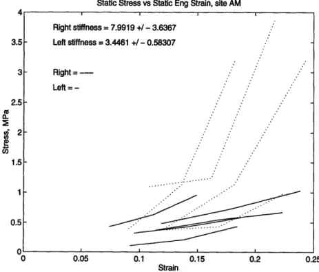
2.3.2 Static Stiffness

The static stress-strain curves are pictured in Figures 2.5 and 2.6 below for the three sites. To determine the static stiffness for the left and right joints, the slopes (i.e. the equilibrium

modulus) of these lines were calculated between the 25 um and 37 um displacements. The mean and standard error of the slopes at each site were computed and compared (Figure 2.5).

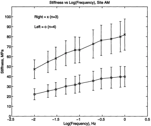
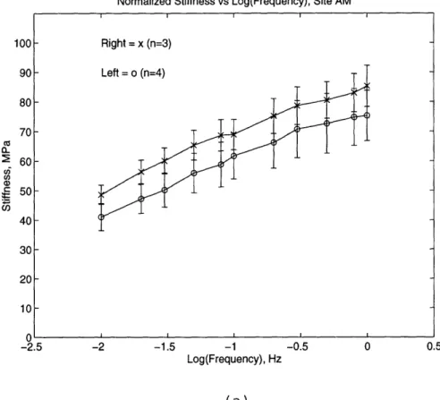
2.3.3 Dynamic Stiffness

For the dynamic stiffness (Figures 2.7 amd 2.8), the trend of left and right joints versus frequency was plotted at each site. Each line represents the mean of one subgroup, and the magnitude of the error bar is one standard deviation.

Static Stress vs Static Eng Strain, site AM

.5 1. 0. .5 5 I, 0.05 Strain 0.15 0.25

Figure 2.5 The static stress-strain curves for the anterior medial site.

Right stiffness = 7.9919 +/ - 3.6367

Left stiffness = 3.4461 +/ - 0.58307

Right =

---Left =

(21)

3. 2. 0. It 5 5 5 n 0.05 Strain 0.15 0.25

(a)

3.5 0.5

Static Stress vs Static Eng Strain, site ML

0.05

Strain

0.15 0.25

(b)

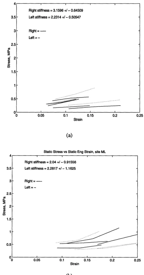
Figure 2.6: The static stress-strain curves for (a) middle medial and (b) middle lateral sites.

I

Right stiffness = 3.1596 +/ - 0.64509 - Left stiffness = 2.2314 +/ - 0.50547 Right=Left = -Right stiffness = 2.04 +/ -0.91556 Left stiffness = 2.2817 +/ - 1.1625 Right = ---Left = -... ... a .. . . .. . . . . . I I I ! E

(22)

-100 90 80 70 M 60 () • 50 40 30 20 10 n

Stiffness vs Log(Frequency), Site AM

Riaht = x (n=31

-2.5 -2 -1.5 -1 -0.5 0 0.5

Log(Frequency), Hz

Figure 2.7: The dynamic stiffness vs frequency for the anterior medial sites of the left and right joints.

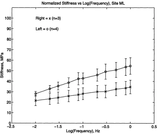
The dynamic stiffness was then normalized to the static stress upon which the dynamic load was superimposed (Figure 2.9 and 2.10). Since the thickness of the tissue varies widely from site to site and animal to animal, the static load also varied. This difference could have an effect on the dynamic load readings. Therefore, the dynamic stiffness was normalized by dividing by the static stress for each data set.

L

(23)

Stiffness vs Log(Frequency), Site MM 100 90 70 50 20 10 -2.5 -2 -1.5 -1 -0.5 0 Log(Frequency), Hz (a)

Stiffness vs Log(Frequency), Site ML

1 Aft3 120 100 -2.5 -2 -1.5 -1 -0.5 0 Log(Frequency), Hz (b)

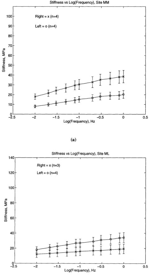
Figure 2.8: The dynamic stiffness versus frequency for the (a) MM and (b) ML sites. Right = x (n=4) Left = o (n=4) ± -.. Right = x (n=3) Left = o (n=4) U E -E - 1-E

(24)

Normalized Stiffness vs Log(Frequency), Site AM

-2.5 -2 -1.5 -1 -0.5 0 0.5

Log(Frequency), Hz

(a)

Normalized Stiffness vs Log(Frequency), Site MM

100 90 80 70 60 50 40 30 20 -2.5 -2 -1.5 -1 -0.5 0 Log(Frequency), Hz

(b)

Figure 2.9: The normalized dynamic stiffness versus frequency for the (a) MM and (b) ML sites.

Right = x (n=4) Left = o (n=4)

(25)

-Normalized Stiffness vs Log(Frequency), Site ML 100 90 80 70 2 60 Co S50 40 30 20 10 n -2.5 -2 -1.5 -1 -0.5 0 0.5 Log(Frequency), Hz

Figure 2.10: Normalized siffness versus frequency for the ML site.

2.3.4 Streaming Potential

To plot the streaming potential, the voltage was normalized by the dynamic strain. Therefore, the units of the y-axis are in milli-volts per percent strain. In Figure 2.11 and 2.12, these values are plotted for the range of frequencies tested.

As before, the streaming potential data was normalized by the static stress over which the sinusoidal displacement was applied (Figure 2.12b and 2.13).

I I

- Right = x (n=3)

- Left = o (n=4)

-2

(26)

Streaming Potential vs Log(Frequency), Site AM 0.08 0.06-, 0.04 > 0.02-cr -0.02 E -0.06 -0.08 -0.1-2.5

-2.5

-2 -1.5 -1 -0.5 0 Log(Frequency), Hz

(a)

Streaming Potential vs Log(Frequency), Site MM

-2.5 -2 -1.5 -1 -0.5 0 0.5

Log(Frequency), Hz

(b)

Figure 2.11: The streaming potential per percent strain vs frequency for the (a) AM, and (b) MM sites. Right = x (n=4) Lnft= n In=41 · · · · ,,_{... 1} Vi J

(27)

Streaming Potential vs Log(Frequency), Site ML

2.5 -2 -1.5 -1 -0.5 0

Log(Frequency), Hz

(a)

Normalized Streaming Potential vs Log(Frequency), Site AM

-2 -1.5 -1 -0.5

Log(Frequency), Hz

0 0.5

(b)

Figure 2.12: The streaming potential per percent strain versus frequency (a) for the ML site and (b) the normalized streaming potential per percent strain versus frequency for the AM site.

I I Right = x (n=3) Left = o (n=4) 0.1 0.08 0.06 C 0.04 > 0.02 E E 0 0 a. cn-0.02 .c E 2 -0.04- -0.06--0.08 -U..1 Right = x (n=4) Left = o (n=4) 0.35 0.3 0.25 0.2 0.15 0.1 0.05 -0.05 -n i 5 III

- - I

I

-7 -E -.2 -2.•

(28)

Normalized Streaming Potential vs Log(Frequency), Site MM '.5 -2 -1.5 -1 -0.5 0 0.4 0.35

0.3

0.25 0.2 0.15 0.1 0.05 0 -0.05--U.1 -2 fl4

0.35

0.3

Figure 2.13: the ML site. 0.25 0.2 0.15 0.1 0.05

0--0.05 -n1 I Log(Frequency), Hz

(a)

Normalized Streaming Potential vs Log(Frequency), Site ML

-2.5 -2 -1.5 -1 -0.5 0

-2.5 -2 -1.5 -1 -0.5 0

Log(Frequency), Hz

(b)

The normalized streaming potential per percent strain for (a)

0.5

the MM site and (b)

Right = x (n=3) Left = o (n=4)

(29)

2.3.5 Thickness

The thickness was measured for the three sites and separated into left and right subgroups (Figure 2.14). The bar represent the mean thickness for the subgroups. The magnitude of the error bars is plus and minus one standard deviation.

2.4 Discussion

2.4.1 Static Stiffness

The Student's (two-way) T-test indicated that there was no significant difference between the static stiffnesses of the left and right joints (P = 0.2061 for the AM site , P = 0.2872 for the MM

site, and P = 0.8737 for the ML site).

Thickness by Site

0 1 2 3 4 5 6 7

site

Figure 2.14: The means and standard right joints separated.

deviations of thickness for the three sites with left and · rrr

(30)

2.4.2 Dynamic Stiffness

The Student's T-test revealed no significant difference at all sites between the left and right joints for the dynamic stiffness measurements (Figures 2.7 and 2.8).

Since the experiments were performed under displacement and not load control, figures 2.7 and

2.8 represent dynamic load responses at different static stresses (possibly due to a difference in

the amount of preload applied to the joint prior to the experiment). To normalize the dynamic stiffnesses, the dynamic stiffnesses were divided by the static stresses to which the dynamic displacements were added. With the normalized data, no statistically significant left/right differences were found at any site.

2.4.3 Streaming Potential

For the streaming potential measurement, the T-test showed no significant difference between left and right joints. After static stress normalization (see 2.4.2), the T-test again showed no left/ right difference.

2.4.4 Thickness

T-tests on the thickness measurements revealed no left/right differences at any of the three sites (P = 0.44 for the AM site, P = 0.29 for the MM site, and P = 0.81 for the ML site). The

differences between the three sites were also examined. The AM and ML sites did not show statistically significant differences in thickness; however, the MM site was distinctly thicker than the AM and ML sites. Since the lesion is located at the MM site, this thickness difference warrants further examination in the future.

2.4.4 Sources of Error

For several of the tests, the standard deviation was quite high due to the low number of samples and the learning curve of the experimental protocol. In many of the plots, there is a difference between the means of the left and right joints; however, in most cases the means are within the standard deviation of the two subgroups.

(31)

One source of error is the difference in preload applied to the joint prior to the experiment. In most cases, this preload ranged from 10-30 grams. However, it is difficult to tighten up this range because we are unsure of the point at which the indentor probe begins to deform the cartilage. Also, since the cartilage is so thin, it is physically difficult and time-consuming to consistently preload before the experiment. The re-normalization of our dynamic stiffness and streaming potential values should decrease but not eliminate this error. Of course, joint-to-joint and animal to animal variability in these cartilage electromechanical properties contribute to the error.

During Phase 2, this preload value was more carefully monitored. A potential solution is to run the experiment in load control instead of displacement control (Appendix A)

2.4.5 Possible Bias in Testing

One interesting trend is that the mean static and dynamic stiffnesses are consistently higher on the left ML sites and the right AM and MM sites. This trend could indicate a bias in the testing procedure, since the joint is normally positioned in the chamber with the posterior side toward the experimenter. Since the joint chamber has five, rather than six, degrees of freedom, the left and right joints might not be positioned exactly the same when a given site is tested.

Because of this possible bias in our experimental process, we tested one of the Phase 2 joints in its normal position first, rotated the chamber 180 degrees so that the anterior site faces the experimenter and re-ran the experiment. This procedure and the results which indicated no obvious bias are discussed in Appendix B.

2.5 Conclusion

In analyzing the data from the left/right difference experiments, several weaknesses in the testing protocol have become apparent. The potential bias of our testing apparatus mentioned above in section was resolved (Appendix B). Additionally, the difficulty of maintaining a consistent preload must be eliminated, possibly by switching to load control instead of

(32)

displacement control. Changing to load control turned out not to be feasible because of the additional time constraints it imposes (Appendix A). In view of the impracticality of load control and the apparent lack of any physical bias in the system, we proceeded to Phase 2 with relatively small changes in the testing protocol.

(33)

Chapter 3 Electromechanical Differences Between Age Groups, Phase 2

3.1 Introduction

The purpose of the second phase was to determine, first, any changes in electromechanical prop-erties between different age groups of guinea pigs; second, any changes in biochemical proper-ties; and third, any correlation between the two.

After looking at the results of Phase 1, the experimental protocol was altered to make more eco-nomical use of testing time and to add more detail to the static measurements. Otherwise, the dynamic measurements of Phases 1 and 2 were taken essentially the same way. Also, during Phase 2, possibility of changing to Load Control from Displacement Control was explored and rejected. The results of that experiment are presented in Appendix A.

This chapter covers only the electromechanical testing part of Phase 2 since, as was mentioned in Chapter 1, the bulk of the biochemical assays have yet to be performed; however, preliminary bio-chemical assays are discussed in the next chapter. Overall, for the dynamic (normalized and unnormalized) and static stiffness tests, differences in site but no differences in age were found at the 95% significance level. The ANOVA revealed a statistically significant difference for both site and age for the normalized streaming potential data (P=0.043) though post hoc analysis did not show dignificance at a 95% leve. For the thickness measurement, a difference exists for both age and site.

(34)

3.2 Methods and Materials

A total of 45 legs (15 per age group of 3, 8, and 12 months) were received from Procter & Gam-ble. All joints tested were from the right legs. Procter & Gamble kept the left legs for histological

studies. The guinea pig legs were dissected and the thickness was measured in exactly the same manner described in the previous chapter. This part of the study was blind in that Procter & Gam-ble did not inform us of the groupings of the joints until the electromechanical experiments were completed.

All the physical testing apparatus and the inhibitor solutions remained constant between Phase 1 and Phase 2. The major changes were the reduction of the stress relaxation period and the addi-tion of eight more static loads to give more detail to the static compression characteristics of the guinea pig cartilage.

3.2.1 Stress Relaxation

In Phase 1 testing, the cartilage was allowed to stress relax for about 15 minutes. Because a total of 45 joints were to be tested, cutting down the stress relaxation time would allow us to test two joints a day instead of only one. After examining the exponentially decaying static load response, the time constant was determined to be approximately 30 seconds (Appendix D). This is consis-tent with the fact that the cartilage is very thin, and the relaxation time is proportional to the square of the thickness. Instead of a relaxation time of 15 minutes, the time chosen was six times the time constant or about 3 minutes.

3.2.2 Static Stiffness Tests

As can be seen in the static stiffness plots in the previous chapter, the tests did not reveal much detail since the curves consisted of only three points. In order to add more resolution and thereby get a better sense of the region where the stress-strain curve becomes non-linear, eight more static displacement points were added. Instead of displacements of 25, 37, and 42 um, the Phase 2 joints were tested for displacements of 5, 12.5, 20, 25, 20, 37.5, 45, 50, 55, 60, 65, 70, and 75 um.

The cartilage was first indented to 5 um, allowed to stress relax for three minutes, indented to 12.5 um, etc., until the displacement reached 37.5 um at which time the cartilage was dynamically

(35)

stimulated as in Phase 1. After the dynamic measure was taken, the joint was further tested at progressively increasing static displacements. After all static tests for a joint were completed, the thickness was measured at the testing site.

3.3 Results

3.3.1 Number of Samples

Although all 45 joints were electromechanically tested, due to a computer error, the electronic form of the data obtained from 14 joints was lost. Fortunately, the chart recordings of the data were always printed during the experiments and some (4 to 10 joint/site sets) of the data was retrieved from the 14 joints.

3.3.2 Age-Group Code

After the experiments were completed, the age-groupoing code was broken: G3 = 3 months, G1 = 8 months, and G2 = 12 months.

Static stress vs strain, site AM

G1 = ... n=13

G2= .. n= 11

G3= n=11

Strain, percent

Figure 3.1: The stress-strain curves at the AM site for the three age groups. ·

/

(36)

Static stress vs strain, site MM G1 stiffness = 1.5197 +/ - 0.20811 G2 stiffness = 1.5651 +/ - 0.28663 G3 stiffness = 1.3697 +/ - 0.14967 G1 = ... n = 13 G2= ._. n=12 G3 = n = 11 . I .. 0 0.1 0.2 0.3 0.4 0.5 0.6 Strain, percent 0.7 0.8 0.9 1

(a)

Static stress vs strain, site ML

Co a_ 9D G1 stiffness = 1.1685 +/ - 0.27208 G2 stiffness = 1.467 +/ - 0.26549 G3 stiffness = 1.7159 +/ -0.51111 0 0.1 0.2 0.3 0.4 0.5 0.6 Strain, percent G1 = ... n=13 G2 = ._. n = 13 G3= n=12 0.7 0.8 0.9 1

(b)

Figure 3.2: The static stress-strain curves for the (a) MM and (b) ML sites. 8 c 6 (0 4 2 (I . . ..· i I ·

(37)

3.3.2 Static Stiffness

To calculate the static stiffness in the curves in Figures 3.1 and 3.2, the first 6 points were taken, a line was fit to them (least squares method) and the slope computed. The first six points represent the stress vs strain curve between 5 um and 37.5 um displacement. The mean and standard errors of the slopes were calculated and compared at each site and for each age group.

3.3.3 Dynamic Stiffness

For the dynamic stiffnesses (Figures 3.3 and 3.4), the trend of the different age groups versus the logarithm of the frequency was plotted at each site. Each line represents the mean of each group and the magnitude of vertical bars represent plus or minus one standard error at each frequency.

The dynamic stiffness was then normalized to the static stress upon which the dynamic load was superimposed as was done in Phase 1 (Figures 3.5 and 3.6). The justification for the normaliza-tion is discussed in Appendix C.

Stiffness vs Log(Frequency), Site ML

50 40 30 20 -2.5 -2 -1.5 -1 -0.5 0 Log(Frequency), Hz

Figure 3.3: The dynamic stiffness versus frequency plot for site ML.

G1 = X; n = 13 G2= O; n= 11 G3= +; n= 12 It I · · · U _VI I I I -E

(38)

Stiffness vs Log(Frequency), Site MM

-2 -1.5 -1 Log(Frequency), Hz

-0.5 0 0.5

(a)

Stiffness vs Log(Frequency), Site AM

60 50 _ 40 30 20 10 -2 -1.5 -1 -0.5 0 Log(Frequency), Hz (b)

Figure 3.4: The dynamic stiffness versus frequency plots for the (a) MM and (b) AM sites.

G1 = X; n = 13 G2 = O; n = 12 G3= +; n= 11 60 n d& 0 'p v-B 30 U) 20 A -2.5 |1I

--E Ca E L

(39)

Normalized Stiffness vs Log(Frequency), Site ML 11 100 90 80 c 70 0 0 60 i 50 40 30 20

10A

-2.5 -2 -1.5 -1 -0.5 0 0.5 Log(Frequency), Hz

(a)

Normalized Stiffness vs Log(Frequency), Site MM

110 1 1 100- G1 = X; n = 13 G2 = O; n =12 100 GIXn13 -u -80 . 70 0 60 • 50 40 30 20 02.5 -2 -1.5 -1 -0.5 0 0.5 Log(Frequency), Hz

(b)

Figure 3.5: The normalized dynamic stiffness versus frequency at the (a) MI and (b) MM sites.

I i i I

G1 = X; n= 13 G2= O; n= 11 G3= +; n= 12

(40)

Normalized Stiffness vs Log(Frequency), Site AM 100 90 80 70 60 30 -2.5 -2 -1.5 -1 -0.5 0 Log(Frequency), Hz

Figure 3.6: The normalized dynamic stiffness versus frequency at site AM.

3.3.4 Streaming Potential

Streaming potential was plotted normalized by the dynamic strain as was done in Phase 1 (Figures 2.8 and 2.9a). As with the dynamic stiffness graphs, the streaming potential was normalized by the static stress over which the sinusoidal displacement was applied (Figures 3.8b and 3.9).

t-I--E

E

(41)

Streaming Potential vs Log(Frequency), Site ML

-2 -1.5 -1 -0.5 0

Log(Frequency), Hz

(a)

Streaming Potential vs Log(Frequency), Site MM

-2 -1.5 -1 -0.5 0

Log(Frequency), Hz

(b)

Figure 3.7: The streaming potential per percent strain at the (a) ML and (b) MM sites.

0.04 0.03 0.02 0.01 G1 = X; n = 13 G2 = O; n = 11 G3= +; n= 12 _n rt_-2.5 -2.5

K

G1 =) G2=( G3 = n 0.04 0.03 0.02 0.01 .-n n 5 n0 · · · · I I -. 2 -2.= n ~r I I E L

I

(42)

Streaming Potential vs Log(Frequency), Site AM

-2 -1.5 -1 -0.5 0

Log(Frequency), Hz

(a)

Normalized Streaming Potential vs Log(Frequency), Site ML

G1 =X;n=13 G2= O; n= 11 G3= +; n= 12 I II T -±zzir -2 -1.5 -1 Log(Frequency), Hz -0.5

Figure 3.8: The (a) streaming potential per strain versus frequency at site ized streaming potential per strain versus frequency at site ML.

AM and (b) the

normal-0.05 0.04 0.03 0.02 0.01 -- 2.5 -2.5 G1 = X; n =13 G2 = G3 = 0.08 0.06 0.04 0.02 -2.5 II· II'1 I I I I I -· · -H -00A1 E

(43)

Normalized Streaming Potential vs Log(Frequency), Site MM 0.08 0.06 0.04 0.02 -2.5 0.1 n A08 -2 -1. --. -2 -1.5 -1 -0.5 Log(Frequency), Hz

(a)

0 0.5

Normalized Streaming Potential vs Log(Frequency), Site AM

5 -2 -1.5 -1 -0.5 0

Log(Frequency), Hz

(b)

Figure 3.9: The normalized streaming potential per strain versus frequency at the (a) MM and (b) ML sites. Gi = G2=( G3=-I -n G1 =X;n=13 G2= O; n = 11 G3= +; n= 10 0. E - 0.06 0.04 E 7 0.02 A002 no

I

- - -

-I I i 7 1-I Z -2.

(44)

3.3.5 Thickness

The thickness was measured at each of the three sites on each joint (Figure 3.10). The bars repre-sent the mean thicknesses for each group and site and the vertical lines reprerepre-sent plus and minus one standard error.

Thickness by site and age group

Bars 1-3 = site AM; G1-3; n = 13, 12, and 10. Bars 4-6 = site MM; G1-3; n = 13, 12, and 12. Bars 7-9 = site ML; G1-3; n = 13, 13, and 14.

T

I

7V

T T

T

1 2 3

I

T

4 Groups of 5 6

joints by site and age

7 8 9

T

Figure 3.10: A bar graph of the cartilage thicknesses at three sites and age groups.

3.4 Discussion

3.4.1 Static Stiffness

An two-way Analysis of Variance (ANOVA) was performed by age and site for all electrome-chanical measures taken at a 95 % significance level. The results for the static stiffness data show that static stiffness varies by site, but not age (site: P = 0.2313, age: P = 0.1610) with no

interac-0UU 450 400 350 300 250 200 150 100 50 I m

11 J_

I

E T | 1 -E E -E m

(45)

tion effects (P = 0..2313). The Tukey and Student-Newman-Keuls Tests showed that the AM site was significantly stiffer than the other two sites. This result is visually apparent in Figures 3.1 and 3.2 since the curves in Figure 3.1 are so much steeper than in the other two graphs. The higher stiffness at the AM site could be due to effects from the thinner cartilage in that area.

3.4.2 Dynamic Stiffness

An ANOVA on the dynamic stiffness data showed no significant difference due to age, but a vari-ablity due to site with little interaction effects (site: P= 0.0001, age: P=0.3303, interaction:

P=0.6165). The Tukey and Student-Newman-Keuls test showed site AM with a higher stiffness.

After normalization, the ANOVA results were the same (site: P = 0.087, age: P = 0.0717, interac-tion: P = 0.8753). Post hoc analysis revealed that the ML site was stiffer.

3.4.3 Streaming Potential

The ANOVA of the streaming potential data showed a difference by site, and again, no difference by age (site: P = 0.0066, age: P = 0.0830, interaction: P = 0.0755). After normalization by static stress, there is both an age and a site difference (site: P = 0.008, age: P = 0.0427, interaction: P =

0.0643). Although the ANOVA revealed a difference, neither the Student-Newman-Keuls nor the Tukey Test showed a significant difference with age at each site at the 95% level. Clearly, from Figures 2.8 and 2.9, the ML site exhibits the lowest streaming potential as was confirmed by post hoc analysis.

The lower streaming potential at the ML site is most probably related to the relative thinness of that site to the AM and MM sites. Also, it is important to note that when retrieving the lost com-puter data from the paper plots, some of the streaming potential data was unretrievable due to an

streaming potential that was too small to be detected visually. Since most of the irretrievable streaming potential data was at the ML site, the results shown in Figures 3.7a and 3.8bcould actu-ally be skewed too high.

(46)

3.4.4 Thickness

A two-way ANOVA revealed a significant difference with both age and site with little interaction effects (age: P = 0.0079, site: P = 0.001, interaction: P = 0.5421). The Student-Newman-Keuls and Tukey Tests confirmed these results showing that age group 3 (3 months) is the thinnest and the MM site is the thickest. This comes as no surprise since from Watson's MRI experiments, the younger guinea pigs appear to have the thinnest cartilage (Watson 1996).

3.5 Conclusion

The statistical analyses performed to date did not show significant age related changes with the exception of the normalized streaming potential (by ANOVA only). The relatively large standard error may be associated with the indentor-joint geometry, the thickness of the cartilage, and the natural variations between animals. We note, however, that the data on stiffness and streaming potential should be further correlated (normalized) to the biochemical measures on a joint-by-joint basis. These biochemical assays are now in progress. Based on those results, we will be in a

better position to know whether more animals in each age or a wider range of ages may be neces-sary to best characterize the changes in physical and biochemical properties of this guinea pig car-tilage OA model.

(47)

Chapter 4 Biochemical Assays

4.1 Introduction

As mentioned in Chapter 1, Glycosaminoglycans (GAGs) play a major part in giving articular car-tilage its tensile strength. The GAG content of carcar-tilage is also strongly related to the strength of the streaming potential. In studies of the bovine cartilage of OA, small cylindrical disks of articu-lar cartilage are tested electromechanically in a geometrically simple compression chamber. The sample is then assayed for GAG content and the GAG to wet or dry weight ratio is reported. The central difficulty in replicating this technique in guinea pigs is one of joint and tissue size. The task of harvesting a uniform cylindrical plug of cartilage is virtually impossible; therefore we try to shave off with a scalpel as much cartilage from the joint surface as possible. Since the resulting sample is still very small and the tissue water content is therefore difficult to measure, it is difficult to standardize the GAG content by normalization to wet weight.

A potentially more definitive approach is to normalize GAG content in cartilage is by total col-lagen content, since the colcol-lagen content remains fairly constant. It is relatively simple to mea-sure the amount of hydroxyproline in cartilage. Since hydroxyproline is a an amino acid

constituent group unique to collagen, the resulting measure of hydroxyproline is proportional to the total amount of collagen in the assayed sample. Therefore, our solution is to assay the same samples for both GAG and hydroxyproline and normalize the former to the latter.

These biochemical assays will be performed on the 45 joints from Phase 2, but to date we have tested our methods on several joints in order to adapt the bovine protocols for use with guinea pig tissue. The ratio of GAG to hydroxyproline was from 5.2 to 5.8 which is well within the expected

(48)

range for bovine samples.

4.2 Methods

4.2.1 Harvesting Samples

After the joint has been dissected and electromechanically tested, it is placed in a -20 OC freezer in a conical vial for storage. Then the joint is removed from the conical vial and defrosted in a bea-ker of PBE at room temperature for 10 minutes.

After defrosting, the joint is placed under a steroscopic dissecting microscope in a large petri dish. The joint is held in one hand so that the tibial plateau is at about a twenty degree tilt to the focal plane of the microscope. From each joint, two samples are taken, the medial side and the lateral side. Starting with the medial side, a #10 blade scalpel is held at a slight angle to the surface of the cartilage. Then the cartilage is shaved off cutting from the outer edge of the plateau to the cen-ter line. All the cartilage from each side is removed and placed in two cryovials and frozen at -200

C.

4.2.2 Papain Digestion

The cartilage samples now must be enzymatically digested before they can be assayed. The stan-dard method is to use papain to digest the samples. After digestion, both the GAG assay and the hydroxyproline assay can be performed on aliquots from the same digest solution; hence, a useful normalization can result.

Papain is a sulfhydryl protease with a wide specificity for proteins. It remains in zymogen form until activated by cysteine. For 10 ml papain solution, 17.6 mg of cysteine is weighed and placed in a 15 ml conical vial. Using sterile technique, 10 ml of PBE is added to the conical and the new solution was sterile filtered (0.22 um) into another 15 ml conical. Finally, 20 ul papain is ali-quoted and the final digest solution mixed by inversion.

(49)

The cryovials containing the cartilage samples are removed from the -200 C freezer. After defrosting for 5 minutes, 0.5 ml of the papain digest solution is added. The cryovials are then heated in a 60 OC water bath for three hours or until the cartilage is completely digested. After incubation, the digested cartilage is again frozen at -200 C.

4.2.4 GAG Assay

This is a general assay for sulfated GAGs. Shark chrondroitin 6-Sulfate from Sigma (C4S is also present in amounts that vary with age) is used as the standard. To make a stock solution of 2 mg/ ml, 20 mg of C6S is added using sterile technique to 10 ml of PBE. We use 7 test tubes for the serial dilutions to make the samples for our standard curve. To six of those tubes, 100 ul PBE is added while the last tube will contain 200 ul of stock solution. Starting with tube containing the stock solution, the standards are serially diluted by aliquoting 100 ul from one tube to the next.

To run the assay, 20 ul of papain digested sample or 20 ul of a standard is added to a 1.5 ml cuvette. Then 2 ml of 1, 9 dimethylmethylene blue chloride (DMMB) dye is added to the cuvette. The optical density at 525 nm is then read using a Perkin Elmer, Lambda 3B spectropho-tometer. Typically, the standardards are read first, then the samples, and lastly duplicates of the standards.

4.2.5 Hydroxyproline Assay

The day before the assay, the papain digested samples are hydrolyzed in 1 ml of 6N HCI (100 ul digest into 9 ul 6N HC1) at 115 C for 16 to 24 hours in a small oven.

Six tubes are set up for the standard curve with final concentrations of hydroxyproline of 0, 0.5, 1.0, 2.0, 3.0, and 4.0 ug/ml from a stock solution of 100 ug/ml. The sample tubes are removed from the oven and cooled to room temperature under running water. The samples are vortexed and then 2 drops of methyl red are added under a fume hood. NaOH is added until neutralised (around 2.0 ml of 2.5 M NaOH). Then 0.5 M HCI is added dropwise until the pink reappears and a few drops of 0.5 M NaOH are added until the straw color returns.

(50)

To bring the salt concentration down, distilled water is added to bring the volume to 15 ml. To a new tube, 1 ml of the solution is transferred. Under a fume hood, 0.5 ml Chloramine-T is added to each tube (both standards and samples), vortexed, allowed to sit at room temperature for 20 minutes. Then 0.5 ml pDAB solution is added while vortexing. The tubes are incubated at 60 C for 30 minutes.

After incubation, the tubes are cooled in water for 5 minutes. The optical density samples and duplicates of the standards are then read at 550 nm.

4.3 Results

A total of three joints (all from 8 month old animals) were tested. Each of those joints yielded a

medial and lateral cartilage specimen for a total of six samples. We have no confidence in the weight of these samples due to varying hydration levels. The GAG assay was performed on all three joints. Only one of those joints was assayed for hydroxyproline.

4.3.1 GAG

The GAG standard curve is shown in Figure 4.1 where the points represent the average of the ODs from two duplicates. The vertical bars represent plus or minus one standard error. A line was fit using the least square method to the first five points of the curve (the linear region). The OD readings of the six samples and the total ug GAG in each sample calculated from the standard curve line are shown below in Table 4.1.

Joint Medial, OD GAG, ug Weight, g Lateral, OD GAG, ug Weight, g

1 0.535 111.0 0.0042 0.442 42.8 0.0038

2 0.514 95.8 0.0038 0.408 17.5 0.0037

3 0.569 136.0 0.0049 0.432 35.1 0.0034

(51)

Elmer, GAG standard curve 1 0.9 0.8 E 0.7 0 0.6 0.5 0.4 n03 -500 0 500 1000 1500 2000 2500

GAG concentration, ug/ml

Figure 4.1: The standard curve from the GAG assay using the spectrophotometer.

4.3.2 Hydroxyproline

The hydroxyproline standard curve is shown in Figure 4.2. Each point represents the average of the ODs from two duplicates. The vertical bars represent plus or minus one standard error. As with the GAG standard curve, a line was fit using the least squares method to the linear region of the standard curve (the first 6 points). Then the concentration of the samples was calculated from that equation and multiplied by 75 since the 0.5 ml sample is diluted 150 times when the OD is taken.

Only joint 1 was assayed (Medial: 19.0301 ug OH-Pro, Lateral: 8.2067 ug OH-Pro). The result-ing GAG to hydroxyproline ratio was 5.8344 for the medial side and 5.2125 for the lateral side. These values are within the expected range for bovine articular cartilage.

(52)

Hypro standard curve 2 1.5 C 0 LO LO 1 0.5 0 I I I I I -5 0 5 10 15 20 25

Hypro concentration, ug/ml

Figure 4.2.: The standard curve from the hypro (hydroxyproline) assay using the spectrophotome-ter.

4.4 Discussion

Although the GAG and hydroxyproline assays described above are fairly standard for use on bovine and other cartilage explants, we had little previous experience using them with smaller

guinea pig samples. Fortunately, for the sample size harvested and the papain digest volume cho-sen, we were able to get preliminary results that were within the readable range of the spectropho-tometer. Also, a reasonable ratio of GAG to hydroxyproline was found (Medial: 5.8, Lateral: 5.2) for the one joint on which both assays were tested.

(53)

One possible source of error is that in harvesting the cartilage, some bone might be included in the sample as well. Bone also contains collagen, and so the collagen normalization might be skewed.

4.5 Conclusion

The preliminary results from the biochemical assays are encouraging enough to begin testing all

45 joints from Phase 2. The protocol described in the Methods section appears to be easily repeat-able with little chance for inconsistency except at the harvesting stage. The results from the bio-chemical analysis should shed more light on the electromechanical data presented in Chapter 3.

(54)

Chapter

5 Future Testing

5.1 Introduction

Phase 1 of this OA animal study showed that no damage to the joint cartilage was produced by the indentor for a wide range of loads from the indentor apparatus. Although the tested sample size was low, the left and right joints did not appear statistically significantly different. However, the results from the electromechanical tests of the three age groups of guinea pig joints from Phase 2 are not yet conclusive. Differences in site were detected but, for the most part, differences in age were not. The biochemical assays must be completed in order to further normalize the streaming potential and stiffness data.

5.2 Phase 3

The rationale behind this step in the project is to determine the age at which the electromechanical properties change most. Conditional on the results from Phase 2 biochemistry, testing a wider range of ages instead of a smaller range might also be helpful. Since the standard errors in the electromechanical experiments were high, perhaps adding more joints at the age groups already tested would better characterize the statistical distributions of the measured parameters and so boost the confidence of the results.

Increasing the sample size should not pose a time-contraint problem since the current protocol described in Chapter 3 allows two joints a day to be tested. Between Phase 1 and 2, more static displacements were added to give more resolution to the static characteristic of the cartilage. For Phase 3, more dynamic frequency sweeps could be added at different static displacements to give more detail to the dynamic character of the joints. The procedure would be much like what was

(55)

done for the joint described in Appendix C in which the normalization method was justified. By increasing the number of dynamic tests, the dynamic stiffnesses between joints could be more easily compared without the normalization factor. Because the consistency of the electromechan-ical testing seems to be at a reasonable level, any additional change in the methods from Phase 2 to Phase 3 is not recommended.

5.3 Conclusion

Although further statistical and biochemical analyses must be performed to verify whether there are significant differences in the physical properties with age, the Phase 1 and 2 studies have developed a clear, well-defined electromechanical testing procedure for guinea pig joints. Also, the preliminary results from the GAG and hydroxyproline assays show that there is a good pros-pect for obtaining crucial biochemical data quickly from a small amount of cartilage. With addi-tional experiments (adding more joints to the three Phase 2 age groups, increasing the number of dynamic stiffness tests, completing the biochemistry), the data will hopefully add to the utility of the Hartley guinea pig OA model for evaluating pharmaceuticals for OA in the near future.

Characterization of the properties of cartilage in the Hartley guinea pig spontaneous osteoarthritis model