HAL Id: hal-01257956
https://hal.archives-ouvertes.fr/hal-01257956
Submitted on 21 Aug 2020
HAL is a multi-disciplinary open access
archive for the deposit and dissemination of
sci-entific research documents, whether they are
pub-lished or not. The documents may come from
teaching and research institutions in France or
abroad, or from public or private research centers.
L’archive ouverte pluridisciplinaire HAL, est
destinée au dépôt et à la diffusion de documents
scientifiques de niveau recherche, publiés ou non,
émanant des établissements d’enseignement et de
recherche français ou étrangers, des laboratoires
publics ou privés.
hydrothermal exit–fluid temperatures at the Lucky
Strike deep–sea vent field, Mid–Atlantic Ridge,
Thibault Barreyre, Javier Escartín, Rob Sohn, Mathilde Cannat, Valérie
Ballu, Wayne Crawford
To cite this version:
Thibault Barreyre, Javier Escartín, Rob Sohn, Mathilde Cannat, Valérie Ballu, et al.. Temporal
variability and tidal modulation of hydrothermal exit–fluid temperatures at the Lucky Strike deep–
sea vent field, Mid–Atlantic Ridge,. Journal of Geophysical Research, American Geophysical Union,
2014, 119 (4), pp.2543-2566. �10.1002/2013JB010478�. �hal-01257956�
Temporal variability and tidal modulation
of hydrothermal exit-
fluid temperatures
at the Lucky Strike deep-sea vent
field,
Mid-Atlantic Ridge
Thibaut Barreyre1,2, Javier Escartín1, Robert A. Sohn2, Mathilde Cannat1, Valérie Ballu3, and Wayne C. Crawford1,3
1
Marine Geosciences Group, Institut de Physique du Globe de Paris, CNRS, UMR 7154, Univ. Paris Diderot, Sorbonne Paris Cité, Paris Cedex 5, France,2Woods Hole Oceanographic Institution, Woods Hole, Massachusetts, USA,3LIENSs, Université
de La Rochelle, CNRS, UMR 7266, La Rochelle, France
Abstract
We deployed autonomous temperature sensors at black smoker chimneys, cracks, and diffuse flow areas at the Lucky Strike hydrothermal field (Mid-Atlantic Ridge, ~37°17’N) between summer 2009 and summer 2012 and contemporaneously measured tidal pressures and currents as part of the long-term MoMAR experiment to monitor hydrothermal activity. We classify the temperature data according to the hydrogeologic setting of the measurement sites: a high-temperature regime (>190°C) representing discharge of essentially unmixed, primary hydrothermalfluids through chimneys, an intermediate-temperature regime (10–100°C) associated with mixing of primary fluids with cold pore fluids discharging through cracks, and a low-temperature regime (<10°C) associated with a thermal boundary layer forming over bacterial mats associated with diffuse outflow of warm fluids. Temperature records from all the regimes exhibit variations at semi-diurnal tidal periods, and cross-spectral analyses reveal that high-temperature discharge correlates to tidal pressure while low-temperature discharge correlates to tidal currents. Intermediate-temperature discharge exhibits a transitional behavior correlating to both tidal pressure and currents. Episodic perturbations, with transient temperature drops of up to ~150°C, which occur in the high-temperature and intermediate-temperature records, are not observed on multiple probes (including nearby probes at the same site), and they are not correlated with microearthquake activity, indicating that the perturbation mechanism is highly localized at the measurement sites within the hydrothermal structures. The average temperature at a given site may increase or decrease at annual time scales, but the average temperature of the hydrothermalfield, as a whole, appears to be stable over our 3 year observation period.1. Introduction
The space-time variability of exit-fluid temperatures measured at deep-sea vent fields provides important information regarding the hydrogeology and subsurface circulation patterns of hydrothermalflow in young oceanic crust. This is critical for understanding thefluid-dynamical interaction between vents and the overlying ocean and to constrain associated heat, mass, and chemicalfluxes. For modeling purposes, hydrothermal systems are often conceptualized as steady-stateflow environments [e.g., Lister, 1980; Cann and Strens, 1989; Sleep, 1991] or as varying [Lowell and Burnell, 1991; Fontaine et al., 2008; Han et al., 2013] over longer time scales than those of thefield observations (e.g., discharge rates and temperatures), which also exhibit significant spatial variability [e.g. Fornari et al., 1998; Lilley et al., 2003; Scheirer et al., 2006; Sohn, 2007a; Larson et al., 2007, 2009].
Time series temperature measurements made at mid-ocean ridge hydrothermal vents have demonstrated two distinct modes of temporal variability: episodic responses to perturbations from tectonic, magmatic, or mineralization processes [e.g., Sohn et al., 1998; Johnson et al., 2000; Sohn, 2007b; Gribbin et al., 2012] and periodic oscillations related to tidal processes [e.g., Kinoshita et al., 1998; Davis and Becker, 1999; Tivey et al., 2002; Jupp and Schultz, 2004; Crone and Wilcock, 2005; Scheirer et al., 2006; Sohn, 2007a].
Crustal permeability and verticalflow velocity, which are difficult to measure in the field, are fundamental parameters of the hydrothermal system [e.g., Wilcock and McNabb, 1996; Jupp and Schultz, 2004; Crone and Wilcock, 2005] and may be constrained from the response of the system to external forcing. On this point,
Journal of Geophysical Research: Solid Earth
RESEARCH ARTICLE
10.1002/2013JB010478
Key Points:
• High-temperature outflow at deep-sea vent dominated by tidal pressure • Lucky Strike displays stability in temp-erature over three years of monitoring • Episodic temperature perturbations
are local and shallow
Correspondence to:
T. Barreyre, [email protected]
Citation:
Barreyre, T., J. Escartín, R. A. Sohn, M. Cannat, V. Ballu, and W. C. Crawford (2014), Temporal variability and tidal modulation of hydrothermal exit-fluid temperatures at the Lucky Strike deep-sea ventfield, Mid-Atlantic Ridge, J. Geophys. Res. Solid Earth, 119, 2543–2566, doi:10.1002/2013JB010478. Received 1 JUL 2013
Accepted 9 FEB 2014
Accepted article online 15 FEB 2014 Published online 2 APR 2014
however, progress has been limited by the paucity of deep-sea vent exit-fluid data and uncertainties over the nature of the perturbation processes [e.g., Lowell and Germanovich, 1994; Germanovich et al., 2000, 2001; Ramondenc et al., 2006].
The existing data also demonstrated that there are broadly two types of hydrothermal venting: focused, high-temperature discharge from chimney structures (>100°C and often between 300°C and up to ~400°C) and diffuse, low-temperature (<100°C) discharge from cracks, through the seafloor, or at mineral deposits [Corliss et al., 1979]. Temperature measurements from sites of focusedflow can be remarkably stable over time periods of up to a few years [Langmuir et al., 1997; Fornari et al., 1998; Scheirer et al., 2006; Larson et al., 2007, 2009], whereas temperature measurements from diffuseflow are much variable [Tivey et al., 2002; Scheirer et al., 2006; Sohn, 2007a]. This difference may result from the two types of discharge being associated with different circulation systems: focusedflow and venting being associated with primary (deep) circulation and diffuse venting being associated with either secondary (shallow) circulation or leaking and mixing of primary fluids. Up until now, however, there have not been enough observatory-style measurements to determine if and how geological factors (e.g., ridge spreading rate, spreading modality, substrate type) and hydrogeological differences impact the nature of hydrothermal discharge.
Long-term (up to several years) temperature measurements have only been carried out at a few, geologically distinct mid-ocean ridge hydrothermalfields: the fast-spreading and volcanically active East Pacific Rise (EPR) at 9°50′N [Fornari et al., 1998; Sohn et al., 1998; Scheirer et al., 2006], the slow-spreading, detachment fault environment of the TAG segment of the Mid-Atlantic Ridge (MAR) [Sohn, 2007a], and the intermediate-spreading Cleft Segment [Tivey et al., 2002] and Main Endeavour Field (MEF) [Larson et al., 2007, 2009] along the Juan de Fuca Ridge (JdFR). Exit-fluid temperature records from all of these experiments have spatially complex episodic variability that is attributed to local geological or hydrogeological processes, and periodic variability at tidal frequencies (which could be caused by the tides themselves or tidally induced currents). All long-term (on the order of a year or more) exit-fluid records from diffuse discharge sites exhibit some degree of periodic variability at tidal frequencies, but the details vary among sites. While poroelastic models predict tidal modulation of discharge velocity and temperature via the propagation of pressure transients into the shallow crust [e.g., Jupp and Schultz, 2004; Crone and Wilcock, 2005], discharge temperatures may also be affected by tidal and inertial bottom currents [JdFR, Tivey et al., 2002; MAR, Kinoshita et al., 1998]. Poroelastic theory predicts that periodic variability at tidal periods should be observed at sites of focused discharge, but, to date, this effect has only been reported at the MEF along the intermediate-spreading JdFR [Larson et al., 2007, 2009]. Exit-fluid temperature variations at tidal periods were observed over an
approximately 2 month observation period for some of the focused discharge sites at the MEF, which were interpreted as resulting from subsurface mixing between non-seawater end-memberfluids at, or just beneath, the interface between crustal layers 2A and 2B (i.e., 550 m under MEF [Van Ark et al., 2007]). Here we report results from a 3 yearfield program to measure exit-fluid temperatures at nine sites from the Lucky Strike hydrothermalfield on the slow-spreading MAR. This experiment benefits from contemporaneous measurements of exit-fluid temperature, bottom pressure, bottom currents, and local seismicity. First, these time series allow us to investigate the nature of temporal variability at sites of focused and diffuse outflow and to consider the hydrogeological implications for deep-sea ventfields and their interaction with the overlying water column. We apply a spectral analysis to objectively determine whether periodic variations of temperature records are forced by tidal currents or pressure. Second, these temperature records provide information regarding discharge stability at individual vent sites and at the scale of the hydrothermalfield as a whole, over a time period of 3 years. Our analysis allows us to refine the hydrothermal discharge model for the Lucky Strike hydrothermalfield, with implications for other basalt-hosted hydrothermal systems within the rift valley of slow-spreading ridge segments.
2. The Lucky Strike Hydrothermal Field
The Lucky Strike hydrothermalfield (LSHF) is located at the summit of a central volcano on the ~80 km long Lucky Strike ridge segment, which extends along the MAR between 37°03’N and 37°37’N (Figure 1a). The central volcano is underlain at 3–4 km depth by an axial magma chamber (AMC) [Singh et al., 2006; Combier, 2007], which is the presumed heat source driving hydrothermal circulation at the LSHF. The southeastern vents have significantly lower Cl/Mg and higher86Sr/87Sr than the northeastern and western vents
[Charlou et al., 2000], which could result from either two chemically distinct hydrothermal cells or phase separation of a similar sourcefluid [Pester et al., 2012]. Microearthquakes at LSHF, interpreted to have a hydrothermal origin, suggest that the maximum depth offluid penetration is ~3 km below the rift valley immediately north of the hydrothermalfield, and somewhat shallower (~2.5km) immediately to the south [Crawford et al., 2013].
(a)
(b)
Figure 1. (a) Location of the main hydrothermal sites (boxed labels) at the Lucky Strike Hydrothermal Field (LSHF), and position of different geophysical instruments installed during Bathyluck’09, MoMARSAT10, MoMARSAT11 cruises: high-temperature probes (circles), high-temperature probes associated with low-temperature probes (triangles), the two MoMAR observatory nodes SEAMON E and W (stars), the pressure gauge (diamond), and the current meter 2009–2010 (square). Names of sites: TE: Tour Eiffel, MS: Montsegur, CI: Cimendef, IS: Isabel, SI: Sintra, WC: White Castle, CY: Cypress, BC: Benchmark C, CR: Crystal, and SC: South Crystal. The contour interval is 10 m. Multibeam bathymetry data from Ondréas et al. [2009]. (b) Photomosaics of the Montsegur (MS, left) and South Crystal (SC, right) sites, and location of temperature sensors. High-temperature probes are indicated by a white square (1 year probe recording) or a white circle (cruise-long probe recording). Low-temperature probes are indicated by a white triangle. Hydrothermal outflow is indicated by white areas (bacterial mats), which allow us to ascertain the geometry offluid exit. X and Y axes are in Universal Transverse Mercator (UTM, meters). Resolution of photomosaic is up to 5 mm/pixel. Photomosaics from Barreyre et al. [2012]. Names of probes are shown“shorter” on the figure for better visibility; H is for high temperature (L for low temperature), and DXX gives year of the deployment. Sensor names corresponding to those reported in Table 2 are as follows. MS: H1D09: HW0007D09, H2D10: HW0014D10, H3D11: HW0020D11, H4D09: HW0009D09, H5D09: HN29007D09, H6D11: HN29014D11, H7D09: HN29013D09, H8D09: HN29014D09, L1D09: LW0004D09, L2D09: LW0001D09, L3D10: LW0005D10, L4D10: LW0002D10, L5D11: LW0015D11. SC: H1D10: HW0006D10, H2D11: HW0018D11, H3D11: HW0005D11, H4D09: HN29010D09, H5D11: HN30008D11, L1D11: LW0014D11, L2D10: LW0004D10.
The LSHF hosts several active hydrothermal sulfide structures, extending over an area of ~1 km2and surrounding
a lava-filled depression 1740 m beneath the sea surface, often referred to as the “lava lake” (Figure 1a) [Fouquet et al., 1995; Ondréas et al., 2009; Humphris et al., 2002; Barreyre et al., 2012]. Extensive video imagery and seafloor image mosaics have revealed that hydrothermal discharge occurs through chimneys, mounds, and surrounding areas of diffuse outflow (i.e., patches, cracks) [Barreyre et al., 2012]. Based on the videographic and photomosaic data, the total heatflux associated with the LSHF is estimated to be between ~200 and 1000 MW, with the major fraction on the east side of thefield, primarily through diffuse flow [Barreyre et al., 2012].
Throughout the LSHF, discharge tends to localize into discrete areas of both diffuse and focusedflow. Image mosaics have been used to constrain the spatial limits of each site [Barreyre et al., 2012; Mittelstaedt et al., 2012]. The discharge zones are often located along fault scarps and fractures associated with the ~1 km wide axial graben that dissects the volcano. In this experiment, we instrumented nine hydrothermally active sites between 2009 and 2012 and obtained complete temporal coverage for four sites and partial coverage for the otherfive. Below we provide a brief description of each study site and the instrumentation strategy (Figure 1a and Table 1).
2.1. Montsegur (MS)
It extends over a 24 m × 16 m area in the SE of the LSHF and features two prominent sulfide mounds. The larger mound, in the north, is 10 m × 15 m and rises>5 m above the adjacent seafloor. The smaller mound, to the south, is 5 m × 6 m and rises ~3–4 m above the seafloor. Both are conical and are emplaced on a flat hydrothermal slab [Langmuir et al., 1997; Cooper et al., 2000; Humphris et al., 2002; Ondréas et al., 2009; and Barreyre et al., 2012] composed of consolidated volcaniclastic material and hydrothermal minerals [Gribbin et al., 2012]. We identified at least seven high-temperature vents in addition to extensive diffuse low-temperature discharge through cracks and the moundsflanks. This site was continuously monitored for outflow temperatures between 2009 and 2012.
2.2. Tour Eiffel (TE)
Located in the SE of the LSHF, it extends over a 24 m × 20 m area. A detailed description of this site and the heatfluxes associated with both diffused and localized flow is available in Mittelstaedt et al. [2012]. TE is dominated by a massive hydrothermal structure that rises ~20 m above surrounding seafloor [Langmuir et al., 1997], located at the edge of a small fault scarp. Diffuseflow is mainly observed both on the walls of the edifice and around a crack network at the base of the hydrothermal structure. During our experiment, the hydrothermal edifice displayed at least eight clearly identified high-temperature vents, in addition to widespread diffuseflow through its surface and cracks. We continuously monitored this site for outflow temperatures between 2009 and 2012.
2.3. Cimendef (CI)
Located ~30 m west of Montsegur in the SE part of the LSHF, this site is emplaced on a hydrothermal slab and covers an area ~5 m in diameter. We identified only one small active chimney (~1 m high) and an associated
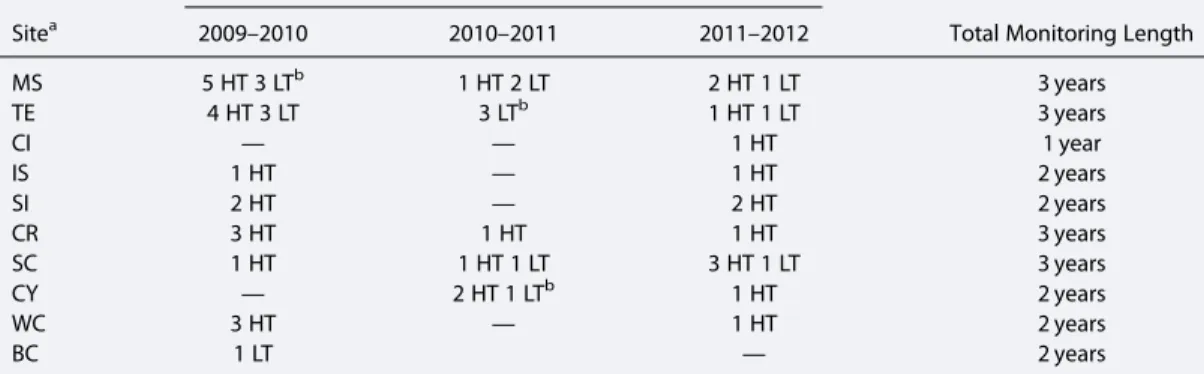
Table 1. Summary of Autonomous Temperature Probe Deployments at Each Site for the 3 Years of Monitoring Deployment Period
Sitea 2009–2010 2010–2011 2011–2012 Total Monitoring Length
MS 5 HT 3 LTb 1 HT 2 LT 2 HT 1 LT 3 years TE 4 HT 3 LT 3 LTb 1 HT 1 LT 3 years CI — — 1 HT 1 year IS 1 HT — 1 HT 2 years SI 2 HT — 2 HT 2 years CR 3 HT 1 HT 1 HT 3 years SC 1 HT 1 HT 1 LT 3 HT 1 LT 3 years CY — 2 HT 1 LTb 1 HT 2 years WC 3 HT — 1 HT 2 years BC 1 LT — 2 years a
Location and names of sites are given in Figure 1 and Table 2, and geological settings and characteristics of the sites are given in section 2.
b
high-temperature vent, in addition to extensive diffuseflow and cracks around the structure. We monitored this site for outflow temperatures in 2011–2012.
2.4. Isabel (IS)
Located ~160 m west of Tour Eiffel in the SE part of the LSHF, this site covers an area ~5 m wide × 8 m long. We identified two small active chimneys (<1 m high) at the base of the edifice and three associated high-temperature vents, in addition to diffuseflow on the flank of the edifice, which is emplaced on hydrothermal slab. We monitored this site for outflow temperatures in 2009–2010 and in 2011–2012.
2.5. Sintra (SI)
This is a massive sulfide complex located in the north of the LSHF extending over an area ~7 m wide × ~5 m high [Langmuir et al., 1997]. High-temperature discharge mainly occurs along the top of a ridge formed by the complex. We identified at least four high-temperature vents, in addition to pervasive diffuse flow through most of the edifice’s surface, which is largely covered by mussel beds. The high-temperature vent Sintra is the only active site in this NNE area of LSHF, and visual inspections suggest that it may be waning (observations from the yearly 2009 through 2012 cruises). We monitored outflow temperatures at this site in 2009–2010 and 2011–2012.
2.6. Crystal (CR)
Located in the west of the LSHF, this site extends over an area ~5 m in diameter. We identified at least three high-temperature vents on two parallel ridges, in addition to limited diffuseflow on these two ridges [Von Damm et al., 1998; Humphris et al., 2002]. A zone of remobilized hydrothermal deposits is located in between the ridges (observations from the yearly 2009 through 2012 cruises). We continuously monitored outflow temperatures from 2009 to 2012.
2.7. South Crystal (SC)
A ~2 m high conical hydrothermal complex located ~25 m SW of Crystal in the west part of the LSHF, it covers an area ~2 m diameter. We identified two high-temperature vents, in addition to an extensive diffuse flow zone and crack network about 7 m south of the mound (observations from the yearly 2009 through 2012 cruises). We continuously monitored outflow temperatures from 2009 to 2012.
2.8. Cypress (CY)
Located in the SW border of the lava lake in the central part of the LSHF, this site extends over an area ~5 m wide × ~10 m long. It includes a diffuseflow zone and several small (<1 m) high-temperature chimney structures. We identified at least three high-temperature vents, in addition to an extensive diffuse flow (observations from the yearly 2009 through 2012 cruises). We continuously monitored outflow temperatures from 2010 to 2012.
2.9. White Castle (WC)
Located in the SW part of the LSHF, this site extends over an area of 5 m × 6 m. We identified four high-temperature vents on the main active ridge, in addition to limited diffuseflow on both flanks, which are mainly composed of remobilized hydrothermal deposits (observations from the yearly 2009 through 2012 cruises). We monitored outflow temperatures between 2009–2010 and 2011–2012.
2.10. Benchmark C (BC)
This site corresponds to the ENE border of the lava lake, where a pressure gauge is installed over a benchmark. Temperature is measured in association with a geomicrobiological colonizator. There are no bacterial mats associated with hydrothermal activity at this site, and these data are used as a reference.
3. Instrumentation, Deployment Strategy, and Data Records
3.1. Instrumentation for Temperature Monitoring
We used four sets of instruments to monitor hydrothermal outflow temperature throughout the LSHF: MISO high-temperature probes, MISO low-temperature probes, NKE S2T6000 probes, and Starmon probes (Figure 2). The instrument-independent consistency of temperature measurements (i.e., repeatability) was assured by both factory and laboratory calibrations.
WHOI MISO high-temperature probes (HW) consist of a titanium body (~10 cm diameter × ~20 cm long), equipped with a ~75 cm-long titanium (Ti) rod. The housing hosts two Omega data loggers connected to a J-Type thermocouple located at the rod tip [Fornari et al., 1994, 1996, 1998]. These instruments can record temperatures of up to 450°C with a precision and resolution of ±1.1°C and 0.21°C, respectively. The sampling interval was typically 24 min for our yearlong records. Each probe contained two loggers for redundancy, with the sampling times offset by 12 min to provide complementary temperature records (see Table 2).
10/14/2010
(a) South Crystal (b) South Crystal 07/03/2011
(d) South Crystal 07/03/2011
(c) South Crystal 10/14/2010
(f ) Cypress 14/10/2010
(e) Montsegur 22/09/2009
Figure 2. ROV dive video frames of probes deployed in 2010 (MoMARSAT10, left) and recovered in 2011 (MoMARSAT11, right) for Figures 2a–2d. (a) Example of high-temperature Woods Hole MISO probe deployment in black smoker at the South Crystal sulfide mound. (b) Video frame of the recovery of this high-temperature probe. Note that the vent orifice where HT probe was installed in 2010 has grown a 1 m chimney while probe is still recordingfluid temperatures (see record in Figure 3). (c) Example of low-temperature Woods Hole probe deployment in diffuse crack hosted by South Crystal crack network. (d) Video frame of the recovery of this low-temperature probe. Note that the LT probe is still at the same place as in 2010 during its deployment. (e) Example of a low-temperature Starmon probe (associated to a colonizer) deployment on diffuse outflow at the Montsegur site in 2009. (f) Other example of a low-temperature Starmon probe (associated to a colonizer) deployment on diffuse outflow at the Cypress site in 2010. In Figures 2c, 2d, 2e, and 2f, white bacterial mats and mussels are visible in 2010 and are still present in 2011, indicating continuous outflow through a crack (c and d), and diffuse flow through the seafloor and bac-terial mat (e and f ), as indicated by the corresponding temperature records (Figure 3).
T able 2. Summa ry of Tempe ratu re Records Used in This Study, Deplo ymen t D e tails , A verag e Tempe rature , and Tren ds a Sites Loca tion XUTM/Y UTM (m) Name of Vent/Cr ack T empe rature Reco rd Na me Deplo yement Date (mm/d d/aa) Reco rd Leng th (days) Sampl ing Inter va l (s) MeanT (°C) stdT (°C) Tren d (°C/yr ) MS 564 214 / 4 1 27075 V01 MS_V01_ 090 906_1010 04_HW00 07A* 6/9/2 009 392.795 14 40 312.353 1.384 0.96 MS_V01_ 101 010_1107 06_HW00 14A* 10/10/ 2010 268.967 14 40 310.885 2.195 6.09 MS _V01_ 11070 6_120717 _HW0020 B* 6/7/2 011 376.329 14 40 312.300 2.309 7.34 V02 MS_V0 2_090906 _101004_ HW 0009A 6/9/2 009 392.909 14 40 299.972 1.500 0.92 V03 MS _V03_ 09092 2_10100 4_HN29 007 09/22 /09 106.394 9 0 310.188 2.604 1 0.36 MS_V03 _110710_ 120 717_HN 2901 4* 10/7/ 2011 372.488 9 0 307.817 0.580 1.24 V04 MS _V04_ 09090 6_09092 2_HN29 014 6/9/2 009 16.324 1 0 316.835 0.508 MS _V04_ 09092 2_10100 4_HN29 013 09/22 /09 36.664 9 0 313.755 0.695 C01 MS_C0 1_090907 _101004 _LW00004 * 7/9/2 009 390.824 90 1 67.037 2.710 5.77 C02 MS_C0 2_090907 _101004 _LW00001 * 7/9/2 009 391.326 90 0 29.232 1 4.400 41.70 C03 MS_C0 3_101011 _110706 _LW00005 * 11/10/ 2010 268.450 14 40 11.979 9.388 18.91 C04 MS_C0 4_101011 _110706 _LW00002 * 11/10/ 2010 268.333 14 40 8.642 6.111 2.02 MS_C0 4_110710 _120716 _LW00015 * 10/7/ 2011 293.171 14 40 13.195 8.449 18.19 INC MS_INC_ 09 0922_101 004_LS028 83* 09/22 /09 374.767 18 0 5.337 0.773 0.13 TE 564 216 / 4 1 27184 V02 TE_V02_ 090 905_1010 03_HW00 10B 5/9/2 009 277.674 14 40 318.792 6.175 8.38 V03 TE _V03_ 09090 6_090922 _HN29 006 6/9/2 009 10.764 1 0 304.934 7.037 V04 TE _V04_ 09090 6_090922 _HN29 017 6/9/2 009 16.680 1 0 312.368 0.671 AIS TE _AIS_0909 23_10101 0_HN2 9016b 09/23 /09 40.540 9 0 289.934 7.487 TE_AIS _110720_ 120 716_HN 3001 5 07/20 /11 36.488 18 0 297.122 1.071 C01 T E_C01_ 0909 07_1010 03_LW000 02 7/9/2 009 390.701 90 0 16.753 1 3.939 2 4.64 TE_C0 1_101015 _110702 _LW00001 * 10/15 /10 259.853 14 40 7.670 2.813 6.63 C02 T E_C02_ 0909 07_1010 03_LW000 03 7/9/2 009 297.664 90 0 96.467 1.219 4.17 T E_C02_ 1010 11_1107 02_LW000 03 11/10/ 2010 65.216 14 40 83.067 1 0.139 TE_C0 2_110720 _120716 _LW00011 * 07/20 /11 361.471 14 40 68.633 2 1.454 5 9.37 C03 TE_C0 3_090907 _101003 _LW00005 * 7/9/2 009 389.304 90 0 40.997 3 3.921 6 4.68 INC TE_SEN _101010 _110702_ LN2600 4* 10/10/ 2010 264.817 18 0 5.177 0.340 0.03 CI 564 185 / 4 1 27070 V01 CI_V01_ 1107 10_1207 16_HW001 2A 10/7/ 2011 37.201 14 40 308.814 1.948 IS 564 059 / 4 1 27247 V01 IS_V01 _090923 _101004_ HW 0012B 3/9/2 009 376.111 14 40 297.611 3.574 0.31 V01 IS_V02 _110712_ 12 0718_HW0 001A* 12/7/ 2011 371.745 14 40 303.099 0.229 0.20 SI 564 263 / 4 1 27529 V01 SI_V01 _090906_ 10 1010_HW0 002A* 6/9/2 009 398.178 14 40 207.982 1.155 1.90 SI_V01 _110704_ 12 0714_HW0 009A* 4/7/2 011 374.903 14 40 205.215 1.483 2.65 V02 SI_V02_ 090 923_101 010_HN 29012 b* 09/23 /09 381.974 9 0 207.186 1.218 0.49 V03 SI_V03_ 11070 4_120713 _HN300 09* 4/7/2 011 374.959 9 0 199.966 1.158 1.63 CR 563 640 / 4 1 27384 V01 CR_ V01_09 0907_101 004_HW0 006A* 7/9/2 009 391.176 14 40 331.429 0.548 1.14 CR_ V01_10 1014_110 703_HW0 010B 10/14 /10 31.617 14 40 317.910 2.833 V02 CR_V 02_0909 07_09092 2_HN2 9012 7/9/2 009 14.111 1 0 329.266 1.398 CR_V 02_1107 03_12071 6_HW001 9B* 3/7/2 011 378.272 14 40 331.492 0.906 1.66 V03 CR_ V03_09 0907_101 004_HW0 008A* 7/9/2 009 166.822 14 40 323.971 2.647 1 6.19 SC 563 619 /41 27368 V01 SC_V 01_1010 14_11070 3_HW000 6B* 10/14 /10 261.733 14 40 339.318 0.854 3.19 SC_V0 1_11070 3_110716 _HW0018 A 3/7/2 011 12.433 14 40 339.195 0.188 SC_V 01_1107 16_12071 6_HW000 5B* 07/16 /11 365.977 14 40 334.848 3.226 5.95 V02 SC_V02 _090922 _101010_ HN290 10* 09/22 /09 383.197 9 0 330.375 0.401 1.11 SC_V 02_1107 16_12071 8_HN3 0008 07/16 /11 29.216 9 0 335.682 2.667
WHOI MISO low-temperature minilog probes (LW) have a smaller Ti housing (~2.5 cm diameter × ~11 cm long) and a ~13 cm Ti rod. These instruments are equipped with a single data logger connected to a thermistor located at the rod tip. These low-temperature instruments can record temperatures of up to 125°C with a precision and a resolution of ±0.22°C and 0.025°C, respectively. The sampling frequency was set to 15 min for instruments deployed in 2009 and 24 min for those deployed in 2010–2011 (Table 2). NKE S2T6000 high-temperature probes (HN) consist of a cylindrical Ti housing (12.8 cm length and 2.3 cm in diameter) and a 40 cm long rod. The data logger is connected to a P-T thermistor at the rod tip and can record temperatures ranging between 0°C and 450°C with a precision and a resolution of ±0.5°C (at less than 100°C) and 0.1°C, respectively. Sampling intervals were set at either 90 s or 3 min for the yearlong records, and at 10 s for the weeklong records (see Table 2).
Starmon low-temperature sensors (LS), which were designed to measure ambient bottom water temperature in the proximity of diffuse outflow, have a cylindrical (2.5 cm diameter × 10.8 cm long) Ti housing with a thermistor located at the tip of a 1.9 cm long rod. These sensors were installed within microbiological colonizers placed on bacterial mats. The probes are equipped with one data logger, recording temperature at a sampling rate of 3 min and over a temperature range of 0°C to 100°C with a precision and a resolution of ±0.05°C (at less than 40°C) and 0.013°C, respectively.
3.2. Bottom Pressure and Current Monitoring
The pressure and near-bottom current (speed and direction) were monitored during the deployment of the temperature sensors. A Seabird 53BPR pressure gauge was installed, as part of a larger seafloor geodesy experiment to monitor vertical deformation at Lucky Strike volcano [Ballu et al., 2009], on the lava lake near the SEAMON-W EMSO (European
Multidisciplinary Subsea Observatory) observatory node (Figure 1a). The site is near the foot of the western fault scarp bounding the axial graben. The sampling interval was 30 s for the entire observation period (2009–2012), and the accuracy and repeatability are, respectively, 0.01% and 0.005% of full scale (i.e., 4000 m). A NORTEK Aquadopp current meter was deployed 14 m above the seafloor at a site ~60 m E of the TE site in 2009–2010, ~450 m SSE of the TE site in
T able 2. (con tinued ) Sites Loca tion XUTM/Y UTM (m) Name of Vent/Cr ack T empe rature Reco rd Na me Deplo yement Date (mm/d d/aa) Reco rd Leng th (days) Sampl ing Inter va l (s) MeanT (°C) stdT (°C) Tren d (°C/yr ) C01 SC_C 01_10101 4_110703 _LW0000 4* 10/14 /10 261.617 14 40 14.806 1.238 2.20 SC_C 01_11070 3_120716 _LW0001 4* 3/7/2 011 378.590 14 40 13.606 0.865 0.62 CY 563 725 / 4 1 27379 V01 CY_V0 1_101015 _110703_ HN300 08* 10/15 /10 129.014 18 0 292.873 0.977 5.46 CY_V0 1_110704 _120716_ HN300 01* 4/7/2 011 378.139 9 0 300.312 2.383 6.09 V02 CY_V 02_1010 14_11070 3_HN3 0010 10/14 /10 73.625 18 0 291.048 2.721 INC CY_IN C_101 014_1107 05_LN2 7010* 10/14 /10 261.816 18 0 4.873 0.492 0.40 WC 563 717 / 4 1 27255 V01 W C_V01 _090915_ 10 1010_HW0 004B 09/15 /09 30.851 14 40 316.110 0.834 V02 WC_V 02_0909 08_0909 21_HN2 9002 8/9/2 009 13.925 1 0 306.805 0.740 WC_V 02_0909 21_1107 04_HN2 9020 09/21 /09 43.763 9 0 309.458 0.867 V03 WC_V0 3_110704 _120717_ HN300 03* 4/7/2 011 379.477 9 0 311.834 0.237 0.06 BC 563 760 / 4 1 27466 INC BC_I NC_ 09091 5_110701 _LS02886* 09/15 /09 653.519 18 0 4.237 0.078 0.01 a The name of the recor d inclu des the initials of hydrothe rmal site s (see F igur e 1), the date and time of deplo yment, the sens or type (LW, H W ,HN, L N ,LS), a nd serial number .A sterisk behi nd probe names deno tes pro bes tha t wer e used for coh erence cal culat ion sho wn in Figur e 11. R a w te mperat ure records are pub licly availa ble as doi:1 0.1594/P AN GA EA.820 343.
2010–2011, and ~900 m SSE of the TE site in 2011–2012 (Figure 1a). Sampling intervals for the 3 years were set at 10, 3, and 6 min, respectively. Nominal velocity uncertainties are 1.4 cm/s in the vertical direction and 0.9 cm/s for the horizontal direction. Both pressure and current measurements instruments are serviced yearly for calibration.
3.3. Monitoring Strategy
We obtained exit-fluid time series data from 54 probes between September 2009 and July 2012, with record lengths varying from several weeks to about a year (Tables 1 and 2). Temperature sensors were deployed and recovered using the ROV Victor during annual cruises: Bathyluck’09, MoMARSAT’10, MoMARSAT’11, and MoMARSAT’12 (Figure 2). We targeted high-temperature vents (>190°C and up to ~350°C), cracks discharging lower-temperature, shimmeringfluids (<100°C), and bacterial mats associated with low-temperature diffuse fluids (typically <10°C). Fifteen additional instruments were deployed but failed to return data because they were either burned by high-temperaturefluids or lost due to chimney collapse or growth of hydrothermal deposits. Successful deployments yielding data and reported in Tables 1 and 2 are used in this study and represent a combined total of ~36.5 years of recording. Four sites (TE, MS, SC, CR) were instrumented for all 3 years of the monitoring experiment,five sites (IS, SI, CY, WC, BC) were instrumented for 2 years, and one site (CI) was instrumented for only the year 2011–2012 (see Table 1 for details). The raw temperature data are publicly available (doi:10.1594/PANGAEA.820343).
We conducted a nested monitoring approach in order to investigate variability across a spectrum of length scales (field scale, site to site, and site scale) and to provide redundancy in case of instrument failure or loss. At high-temperature vents, the HW and HN sensors were deployed with the sensor tip placed up to 10–15 cm inside the vent orifice in order to minimize variability associated with turbulent mixing of hydrothermal fluids with ambient seawater (Figures 2a and 2b). In lower temperature outflows, the tips of the LW sensors were placed within cracks discharging shimmering water (Figures 2c and 2d). At the microbial mat sites (TE, MS, BC, CY), the tips of the LS were placed in shimmering water at the surface of the mats (Figures 2e and 2f ). Whenever possible, probes were redeployed in the same orifice or crack at each measurement site during the annual site visits (see Table 2 for details).
Instrument installation and temperature record interpretation are coupled with seafloor images derived from photomosaics [Barreyre et al., 2012; Mittelstaedt et al., 2012], allowing us to better understand the spatial relationships among temperature records, and with the overallfluid outflow throughout the site (Figure 1b). Seafloor imagery provides a complete view of actively venting areas, which allow us to determine the association of temperature records with specific venting structures to properly place our observations at the scale of the site, and to evaluate their representativeness.
3.4. Data Preprocessing and Time Series
The autonomous clocks for each probe were synchronized to GPS time before deployment and after recovery, and the timing of each temperature record was corrected assuming a linear drift. The average clock drift for HW probes was ~15 min over 1 year, which is comparable to one sampling interval. Each temperature record was visually inspected and trimmed to remove data acquired after the probe was dislodged from its deployment site. In most cases this corresponds to recovery by the ROV, but in some cases the probes became dislodged (e.g., fell out of the chimney or crack) prior to recovery, as verified by ROV video. A few probes became cemented within the wall of hydrothermal structures or chimneys, and these records display a gradual decay, likely associated with the migration of the hydrothermal conduit (i.e.,flow) away from the probe tip. In such cases we terminated the record prior to the gradual decrease in temperature. In this paper we only present and analyze those portions of the temperature records that faithfully measured exit-fluid temperatures for a period of 10 days or more. The bottom pressure and current-meter records were handled in a similar fashion to the exit-fluid records. The timing was corrected assuming a linear clock drift during the duration of deployments, and the records were inspected for spurious data. While the pressure sensor returned 3 years of continuous data (with yearly services), the current meter returned a complete record for thefirst year (2009–2010) and partial records (~110 days) for the second and third years of monitoring (2010–2011 and 2011–2012), due to data logging issues.
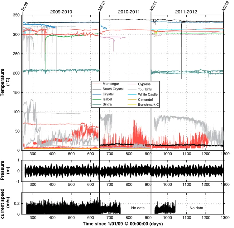
The ensemble set of the 54 temperature records, the bottom pressure record, and the current-meter data used in our analyses are shown in Figure 3. The number of temperature records available for a given time window varies depending on yearly instrumentation strategy, logistical deployment issues, loss of sensors, and truncation of records (see Table 2).
4. Results
The temperature records we acquired from the LSHF can be divided into three categories corresponding to the average temperature and the hydrogeological setting (Figures 3 and 4): (1) High-temperature records acquired from chimneys of focused discharge display average temperatures>195°C; (2) Intermediate-temperature records acquired from cracks discharging shimmeringfluids at average temperatures ranging between ~10°C and 100°C; and (3) Low-temperature records acquired from diffuse discharge zones populated by microbial mats, with average temperatures<10°C (Table 2 and Figures 4a and 4b).
300 400 500 600 700 800 900 1000 1100 1200 1300 0 50 100 150 200 250 300 350 300 400 500 600 700 800 900 1000 1100 1200 1300 0 1 300 400 500 600 700 800 900 1000 1100 1200 1300 0 0.2 -1
Time since 1/01/09 @ 00:00:00 (days)
Temperature (°C) Pressure (m) current speed (m/s) No data No data 2009-2010 2010-2011 2011-2012 BL09 MS10 MS11 MS12 Montsegur South Crystal Crystal Isabel Sintra Cypress Benchmark C White Castle Cimendef
Figure 3. (Top) Plot showing all exit-fluid temperature records from the Lucky Strike hydrothermal field. Vertical lines correspond to the instrument recovery and deployments during cruises: Bathyluck09 (BL09), MoMARSAT10 (MS10), MoMARSAT11 (MS11), and MoMARSAT12 (MS12). (Middle) Pressure data for the monitoring period (conversion from dbars to meters is made using the matlab function sw_dpth, which is based on Fofonoff and Millard Jr. [1983] algorithms). (Bottom) Current-meter speed data for the same time window. The current meter failed between days ~775 and ~900 and between days ~1050 and ~1300.
Figure 4c illustrates differences in behavior for selected temperature records in each of these three categories. High-temperature (HT) records are overall stable and display a low variability; one out of 22 high-temperature records longer than 100 days displays a standard deviation>4°C, while 14 display instead standard deviations of<2°C (<1% of the average temperature). These records typically exhibit unimodal temperature histograms with small (a few °C) deviations (Figure 4c). Intermediate-temperature (IT) records display more complex patterns, with higher standard deviations overall (with a maximum of>30°C), and episodic changes in discharge temperature. This is illustrated in Figure 4c (middle panel), where changes in both the average temperature and the standard deviation appear, yielding a multimodal histogram. Low-temperature (LT)
0 50 100 150 200 250 300 350 0 20 40 60 80 100 0 50 100 150 200 250 300 350 0 1 2 3 4 5 6 7 Count Std % LT regime HT regime IT regime LT regime HT regime IT regime 250 300 350 400 450 500 550 600 650 326 328 330 332 334 Temperature, (¡C) 250 300 350 400 450 500 550 600 650 20 40 60 Temperature, (¡C) 250 300 350 400 450 500 550 600 650 5 10 15 Temperature, (¡C)
Time since 1/01/09 @ 00:00:00 (days)
0 0.1 0.2 0 0.005 0.01 0.015 0 0.05 0.1 0.15 Frequency mean = 330.37 std = 0.40 mean = 29.23 std = 14.40 mean = 5.33 std = 0.77 326 328 330 332 334 20 40 60 5 10 15 High-T Intermediate-T Low-T (a) (b) (c) SC, HN29010 MS, LW00001 MS, LS02883
Figure 4. (a) Histogram of the mean of each of the 54 temperature records, defining the high-, intermediate-, and low-temperature regimes (HT, IT, and LT respectively). (b) Standard deviation normalized by the mean low-temperature in %, calculated for each record, plotted against mean temperature. (c) Examples of high-, medium-, and low- temperature records (top, middle, and bottom, respectively) and their corresponding histograms of temperature, with the frequency normalized by the total number of observations. The mean and standard deviation (std) for each temperature records is also indicated. Sites and names of the probes used as example are given on the top of each panel.
records display average temperatures that are close to that of ambient seawater with low-amplitude (standard deviations of<1°C) continuous variability. While the absolute value of temperature deviations is lower than that observed for intermediate and high-temperature records, they represent up to 25% of the average temperature, compared to<3% for the high-temperature records. LT temperature histograms are unimodal and typically asymmetric (skewed to lower temperatures) (Figure 4c). As described below, these temperature records provide information on the temporal evolution of the LSHF at time scale of months to years (section 4.1) and both episodic and periodic variability on shorter time scales (sections 4.2 and 4.3, respectively).
4.1. Long-Term Evolution of Effluent Temperature
Table 2 reports the long-term temperature trends for all the records used in this study estimated using least squares linear regression. For the 38 records longer than 100 days, the annual trends vary between 65 and +41°C/yr, although most of them (20 out of 38) display trends less than 3°C/yr in magnitude. For the high-temperature records, the range in trends, shown in Figure 5a, is significantly reduced ( 16 to +8°C/yr, 13 out 22 records with trends<3°C/yr in magnitude), with an average of 0.62°C/yr (Figure 5a and Table 2). We
300 400 500 600 700 800 900 1000 1100 1200 1300 0 -2 -4 2 4 300 400 500 600 700 800 900 1000 1100 1200 1300 0 2 4 6 8 10 Number of probes
Time since 1/01/09 @ 00:00:00 (days)
Temperature, (°C) 2009-2010 2010-2011 2011-2012 BL09 MS10 MS11 MS12 0 -20 -15 -10 -5 5 10 15 20 0 1 2 3 4 5 6
Temperature trends (°C/year)
Count
mean = -0.62 °C / year (a)
(b)
(c)
Figure 5. (a) Histogram of temperature trends calculated from high-temperature records spanning over 100 days or more. Vertical black line shows the mean value. (b) Composite average temperature for HT records longer than 100 days and corresponding standard deviation (thin light gray lines) for the 3 year monitoring period and (c) number of temperature records contributing to the composite temperature record. Only composite record sections calculated from six instruments or more, shown in black, are used to infer long-term temperature gradients, while the rest (thick dark gray line) are not considered.
find that the magnitude and even the sign of the temperature trends can vary for records obtained from individual vent sites. For example, the temperature record acquired from vent #1 at Montsegur in 2009 exhibits a positive trend of 0.96°C/yr, whereas the record acquired from vent #2, located 6 m away (Figure 1b), exhibits a negative trend of 0.92°C/yr. Furthermore, vent #1 in Montsegur (Figure 1b, MS), displayed average temperatures and trends for each of the deployments of 312.35°C and 0.9°C/yr in 2009–2010, 310.88°C and 6° C/yr in 2010–2011, and 312.30°C and 7°C/yr in 2011–2012, respectively (Table 2).
Given the variability in long-term trends at individual sites and throughout the wholefield, we have generated a composite temperature record at the scale of the LSHF for each of the deployments. We have selected the HT records from nine studied sites with durations of>100 days (Table 2). We have discarded intermediate- and low-temperature records, which exhibit complex patterns and changes in outflow regime (e.g., Figure 4c). To generate this composite record, we applied a 14 day running medianfilter to each record to remove short-term perturbations. We then removed the mean from each smoothed record. Finally, we average these resulting records to obtain a zero-mean composite temperature record and the corresponding standard deviation (Figure 5b). We note temporal variations in the number of sensors contributing to these composite records (Figure 5c), particularly during recovery and re-deployment. We consider that robust and meaningful estimates of temperature trends can only be obtained from composite records derived from six instruments or more (black line, Figure 5b, black circles, Figure 5c); the remaining records (thick dark gray line in Figures 5b and 5c) are not considered in this analysis. Note that some of the temporal variations of the composite record clearly correspond to changes in the number of instruments (e.g., temperature changes around days 360 and 410 in Figure 5a). The trends obtained for 2009–2010 and 2011–2012 are 0.1 and 0.7°C/yr, and within the observed standard deviation of<2°C (Figure 5b). These values are comparable to the average of individual trends reported in Table 2, which yield 1.6 and 0.6°C/yr for 2009–2010 and 2010–2011 respectively. While it is not possible to derive a continuous composite record for the 3 years of monitoring, the average of trends from individual HT records is<1°C/yr (Figure 5a).
Temporal variability in temperature at longer time scales (up to two decades) can only be derived from historical, discrete temperature measurements from different sites throughout the LS hydrothermalfield. The highest temperatures measured at any given year for each of the sites reported in the literature or measured during recent cruises to the LSHF are given in Table 3. We have excluded anomalously low values, with temperatures of several tens to more than a hundred degrees below historical values, and that we attribute to
Table 3. In Situ Measurements of High-Temperature Outflow at Selected Hydrothermal Vents (see Ondréas et al. [2009] and Barreyre et al. [2012] for Sites Locations) From the Lucky Strike Field (Temperatures in °C)a
1993b 1994c 1996d 1997e 2008fg 2009g 2010g 2011g 2012g Average ± Stdh
Tour Eiffel 325 324 323 324 184g 317 296 325 322 322.8±2.8
Sintra 212 215 222 176 200f 196/217 – 209 203 211.1±7.8
Y3 333 324 328 – 319f 321 – 325 326 325.1±4.6
Statue of Liberty 202 185 – – – Extinct –
Crystal – – 281 – – 327 327 335 – 329.7±4.6 M.7/Cimendef 302 310 – 306 – – – 308CI – 306.5±3.4 South Crystal – – – – – 340 – 342 340 340.7±1.1 White Castle – – – – – 310 313 317 319 314.7±4.0 Isabel – 175 – – – – – 305.6 304 304.8±1.1 Montsegur 303i 310j 318j 294j – 296k 306k 316k 322k 308.1±10.2 a
Numbers in italics correspond to values significantly lower than the average, and that we attribute to measurements within the mixing zone of seawater and hydrothermalfluids.
b
FAZAR cruise [Langmuir et al., 1997].
c
DIVA 1 cruise [Charlou et al., 2000].
d
LUSTRE cruise [Von Damm et al., 1998].
e
Flores cruise [Charlou et al., 2000; Donval et al., 1997].
f
KNOX18RR cruise (data from WHOI Deep Submergence database, JASON VirtualVan available at http://4dgeo.whoi. edu/jason/).
g
This study, from cruises MoMAR (2008), Bathyluck (2009), MoMARSAT (2010, 2011, and 2012).
h
Average and standard deviation do not include the temperatures in italics, which are considered anomalously low.
i, j, k
: Sites at Montsegur: M6 (i), M4(j), and vents measured during MoMAR cruise, reported as Montsegur (k) and that may be distinct from M4 and M6, see Barreyre et al. [2012].
temperature measurements performed within the mixing zone and thus cooler than the high-temperature fluids. At sites monitored for ~20 years (TE, SIN, Y3, SL, CI, and MS), temperatures are very stable and display no apparent or significant decline or increase over time (trends in magnitude <1°C/yr). In the case of Montsegur (MS), this temporal evolution may not be well constrained, as there is ambiguity regarding sites of measurements (M4/U.S.4 and M6/U.S.6 vents, both at Montsegur mounds, see Langmuir et al. [1997]; Von Damm et al. [1998]; Barreyre et al. [2012]). For sites inspected since 2009 and with temperature measurements in the same vent (SC and WC), the temperatures are stable within<5°C of the mean.
4.2. Episodic Variability: Stochasticity of Abrupt Temperature Excursions 4.2.1. High Temperature
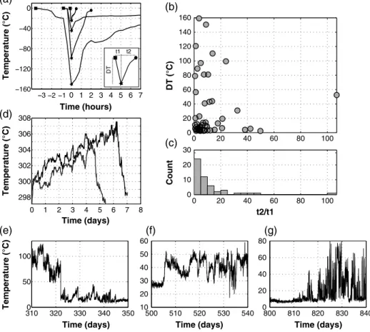
As mentioned above, some of the HT records and most of the IT records exhibit abrupt, episodic, temperature excursions. Episodic perturbations observed in HT records consist primarily of abrupt temperature drops followed by a gradual recovery to the original exit temperature. Figure 6a shows four representative examples from the set of 52 episodic events observed in the HT records, with temperature drops (DT) ranging from 3 to ~160°C from the initial temperature T0. We characterize the events by identifying the time required
to reach the minimum temperature (t1) and then the time required for the temperature to recover 95% of
temperature drop DT (t2). The HT episodic events have typical durations of a few hours (with a few lasting up
to ~2–3 days) with t2/t1typically<20 (70% of t2/t1<10, Figures 6b and 6c). We do not observe any correlation
between the magnitude of the temperature drop with neither the event duration nor t2/t1.
The HT records also display a few temperature increases, as shown in Figure 6d for the Montsegur site in the 2009–2010 deployment. These events are markedly different from the cooling events, and displaying temperature increases of up to 10°C spanning over 4–6 days. In contrast, the temperature drop is sudden and
0 20 40 60 80 100 0 20 40 60 80 100 120 140 160 DT (°C) 0 20 40 60 80 100 0 10 20 30 t2/t1 Count (a) (b) 3100 320 330 340 350 50 100 500 510 520 530 540 10 20 30 40 50 60 800 810 820 830 840 0 20 40 60 80
Time (days) Time (days) Time (days) Temperature (°C) (e) 0 1 2 3 4 5 6 7 8 298 300 302 304 306 308 0 1 2 3 4 5 6 7 0 t1 t2 DT Time (days) Time (hours) Temperature (°C) Temperature (°C) (d) (f) (g) (c)
Figure 6. (a) Four selected examples of cooling events, with the Y axis showing the temperature minus the temperature (T0) before the drop. (b) Plot showing the ratio between the time of recovery to the 95% of the temperature drop (t2)
and the time of the temperature drop (t1) and the corresponding drop of temperature (DT). (c) Corresponding histogram of
the ratio t2/t1. (d) The two warming events that have been observed in HT records. (e, f, g) Three different panels zooms
spans over ~1 day, with the temperature returning to that at the start of the event. Owing to the scarce number of such events, it is not possible to statistically characterize them.
4.2.2. Intermediate Temperature
In Figures 6e, 6f, and 6g, we show examples of 40 day-long IT records displaying both warming and cooling events. Exit-fluid temperatures in the IT records exhibit rapid increases and decreases of up to several tens of °C but with no subsequent recovery to pre-event levels. In Figure 6e, following a sharp drop of ~80°C (black line), there is a succession of warming events with excursions of several tens of degrees and of a shape that is similar to that observed in the HT records (Figure 6d). Figure 6f shows in contrast a warming event followed up by temperature variations spanning over ~20°C, where no clear baseline can be defined. Finally, Figure 6g, a third type of variability in IT records is characterized by recurrent temperature peaks above background seawater temperature (baseline).
4.2.3. Site and Inter-Site Variability and Link With Microseismicity
We illustrate the lack of intra- and inter-sites correlation in the episodic temperature perturbations by showing a ~25 day interval of records from the Montsegur (Figure 7a) and Tour Eiffel sites (Figure 7b). Although the records from each site were acquired from closely spaced sensors at different outflows, there is no relationship
HW010B HW007A HW009A HN29016b LW0005 LW0003 LW0002 LW0001 LW0004 280 285 290 295 300 305 0 50 285 335 T (°C) 280 285 290 295 300 305 0 100 200 300
Time since 1/01/09 @ 00:00:00 (days)
T (°C) Mw=-0.9 Mw=-0.8 Mw=-0.8 Mw=0.1 Mw=-0.6Mw=-0.9 Mw=-0.7Mw=-0.8 (a) (b) MS TE
Figure 7. Examples of high- and low-temperature records installed in MS (a) and TE (b) over a 27 days time window. Names of probes are indicated at the right of the records. Earthquakes with magnitude> 1 and occurring below the field are shown by black stars and dashed lines, together with their magnitude. Note that there is no correlation between variations in the temperature offluid outflow among records, nor with seismicity.
1210 1212 1214 1216 1218 1220 1222 1224 1226 190 192 194 196 198 200 202 204 206 Temperature, (°C)
Time since 1/01/09 @ 00:00:00 (days)
(a) (b) (c)
Figure 8. (a) ROV video frames of two probes (HW0009 at the top of the chimney and HN30009 at the base of the chimney) installed in two different vents from the same chimney structure and deployed in 2011 (MoMARSAT11) and recovered in 2012 (MoMARSAT12, right). (b) Sketch of (a) to indicate the measure points and placement of instruments. (c) Temperature records of probes HW0009 (gray, top of chimney) and HN30009 (black, bottom of chimney).
between the observed variations in discharge temperature. We note that the numerous temperature drops in HT record HN29016b (TE, Figure 7b) are not correlated with any events in the other HT and IT records acquired nearby (horizontal distances of<10 m) at this site. The HT records at the MS site (Figure 7a) are very stable and lack any temperature excursions during this period of time that may be correlated with those observed at TE. Figure 8 illustrates the only instance where we observed correlation of temperature events between two records, one at its summital vent, and the other at a vent a few meters below on theflank of the same chimney at Sintra (Figures 8a and 8b). These records show a periodic, tidal variability of ~0.5–1°C. Over-imposed, there are cooling and warming events that are anti-correlated, and with excursions of up to ~5°C and ~2°C
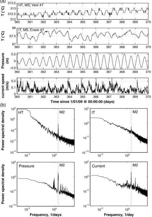
360 361 362 363 364 365 366 367 368 369 370 312 312.5 313 313.5 T (°C) 360 361 362 363 364 365 366 367 368 369 370 67 67.5 68 T (°C) 360 361 362 363 364 365 366 367 368 369 370 5 0 0.5 Pressure (m) 360 361 362 363 364 365 366 367 368 369 370 0 0.1 0.2 current speed (m/s)
Time since 1/01/09 @ 00:00:00 (days)
HT, MS, Vent #1 IT, MS, Crack #1 M2 Pressure Current M2 10 10 100 102 10 10 100 105 (a) (b)
Power spectral density
Frequency, 1/days
Power spectral density
Frequency, 1/day HT M2 IT M2 10 100 10 100 10 100 10 100 10 10 100 105 10 10 10 100 102
Figure 9. (a) Tidal signature illustrated over a 10 day time window on HT and IT records at Montsegur hydrothermal mound (top two plots), and the corresponding variations in bottom pressure and current speed (bottom two plots). (b) Corresponding power spectra for the pressure, current, HT, and IT records shown. Spectral analysis was made by using the multi-taper method described by Thomson [1982]. The frequency of the main semi-diurnal tidal harmonic M2 is shown as gray dashed line. Note that the M2 frequency peak is clearly visible in both temperature spectra but exhibits less power in the intermediate-temperature one.
in amplitude, respectively (Figure 8c). A more pronounced cooling of up to 10°C is observed in both temperature records at day ~1215. This more pronounced cooling event likely represents a perturbation taking place below the two sensors and affecting both of them.
We also document an apparent lack of correlation between temperature events and microseismicity recorded by Ocean Bottom Seismometer (OBS) network deployed contemporaneously [Crawford et al., 2013]. Figure 7 shows the origin time for the eight largest microearthquakes (Mw> 1) observed
in the study area above the melt lens for this time window. None of the microearthquakes affected discharge temperatures at the measurement sites, even taking into account a delay response to the temperature records (4–5 days delay following a seismic event at the EPR [Sohn et al., 1998]). Several HT records lack any temperature excursions and therefore demonstrate that the observed seismicity did not impact the outflow at these sites (Figure 7). Thus, wefind that the episodic temperature variations in the HT and IT records are uncorrelated between measurement sites atfield and inter-site length scales, and they are also uncorrelated with microearthquake activity underlying LSHF.
4.3. Periodic Variability at Tidal Frequencies
All of the temperature records exhibit periodic variability at tidal frequencies as shown in selected HT and IT time series data and spectral estimates (Figures 9 and 10). While the full range of tidal frequencies (fortnightly, diurnal, semi-diurnal, etc.) are found in the pressure and current records, the temperature records only exhibit variability at semi-diurnal frequencies (Figure 9b). We also note the lack of power in the inertial or 4 cpd bands in both current and temperature records. The detailed frequency response at semi-diurnal periods is shown in Figure 10, including the principal lunar semi-diurnal (M2), the major lunar elliptic (N2), the
principal solar (S2), and the luni-solar declination
(K2) frequencies. The four main semi-diurnal tidal frequencies are observed in the HT records (M2, S2, N2, and
K2) and are also visible in the IT records although with an overall lower power (Figure 10). In contrast, both S2
and K2are absent from LT and current records. The amplitude of temperature variations at tidal frequencies is
<0.5°C for the HT records (Figure 9a) and somewhat larger for the LT and IT records. We note that similar semi-diurnal temperature oscillations have been previously reported for IT and LT records from other hydrothermalfields (MEF at JdFR [Tivey et al., 2002]; 9°50’N at EPR [Scheirer et al., 2006]; TAG at MAR [Sohn, 2007a, 2007b]), and for HT records from an additional site (MEF at JdFR, [Larson et al., 2007, 2009]). We evaluated the relationship between tidal processes (pressure and current variations) and the temperature records by conducting cross-spectral analyses using the multi-taper method [Thomson, 1982]. Coherent variability between tidal processes (pressure and current) and the exit-fluid temperature records is restricted to the semi-diurnal band. For tidal pressure, the highest levels of coherency are observed with HT records at
10 10 10 10 10 10 10 10 10 100 101
Power spectral density
Power spectral density
100
Power spectral density
Temperature: M2 N2 S2 K2 M2 N2 S2 K2 M2 N2 S2 K2 Pressure Current HT IT 1.778 Frequency, 1/days
Figure 10. Detail of power spectral density (PSD) plots around the semi-diurnal harmonics peaks for pressure, current, and temperature (HT in solid line and IT in thick gray line). N2 (major lunar elliptic), M2 (principal lunar), S2 (principal solar), and K2 (luni-solar declination) are shown by gray solid lines. Note that S2 and K2 peaks are absent of the current power spectra and are very low amplitude or inexistent in the spectra from the intermediate-temperature record.
the M2frequency, although coherency with HT records is also observed at the N2, S2, and K2tidal frequencies
(Figure 11a, left). IT records show significantly lower coherency at the M2frequency than HT records and lack
coherency at the S2and K2tidal frequencies (Figure 11a, left). For tidal currents, the coherence for the IT
Coherence MS SC TE SI SI CY IS MS WC MS CR SC 0 0.1 0.2 0.3 0.4 0.5 0.6 0.7 0.8 0.9 1 13 14 69 200 205 300 303 308 312 312 331 335 IT Crack HT Vent Pressure Current CY TE TE MS MS SC CY MS SC 0 0.1 0.2 0.3 0.4 0.5 0.6 0.7 0.8 0.9 1 5 5 8 9 12 15 293 311 339 Coherence IT Crack HT Vent Pressure Current 2010 Coherence BC MS MS TE MS SI SI MS CR SC CR 0 0.1 0.2 0.3 0.4 0.5 0.6 0.7 0.8 0.9 1 4 5 30 40 67 207 208 312 324 330 331 IT Crack HT Vent Pressure Current 2009 Temperature vs Current Frequency, 1/days Temperature vs Pressure 0 0.2 0.4 0.6 0.8 1 Coherence 1.85 1.9 1.95 2 0 0.2 0.4 0.6 0.8 1 1.85 1.9 1.95 2 Frequency, 1/days
HT
IT
HT
IT
(a) (b) M2 N2 S2 K2 N2 M2 S2 K2 2011Figure 11. (a) Examples of coherence calculation between both high- (black) and intermediate-temperature (gray) and pressure (left) and current (right). Circles indicate coherence with pressure at the M2 frequency, while triangles indicate the coherence with current at the same frequency. Zero significant level (zsl), calculated for 90% confidence, is shown by a black dashed line on both subplots. Semi-diurnal harmonics N2, M2, S2, and K2 are shown by thin vertical lines. (b) Coherence for selected records (2009–2010, 2010–2011, and 2011–2012) with pressure (black circles) and current (white triangles). Temperature records are arranged by increasing average temperature (indicated below) with names of sites where probes were, and black lines show separation between high-, intermediate-, and low-temperature records. Records used in coherence calculations are indicated in Table 2 with an asterisk behind probe names.
records is similar to that with the pressure and lack coherency at the N2constituent (Figure 11a, right). HT
records exhibit lower coherency with currents than with pressure but display coherency peaks at the N2, S2,
and K2constituents (Figure 11a, right).
Figure 11b reports the set of coherency estimates at the M2frequency between discharge temperature and
both tidal pressure and current for different sites throughout the LSHF for each of the three annual deployment intervals (coherency estimates for 2010–2011 and 2011–2012 limited to ~110 days of data owing to logging issues, as described in section 3.4). These data demonstrate that semi-diurnal variability in the HT records is in all cases significantly more coherent with tidal pressure than tidal current.
By contrast, the results for the IT and LT records are less systematic. Coherency levels for IT records are consistently lower than those observed for HT records for both pressure and currents, with some records showing higher coherency with pressure, others with currents, and the remaining displaying indistinguishable coherency. We only have coherency estimates for four LT temperature records (installed over algal mats, Figures 2e and 2f): two from the 2009–2010 deployments at MS and BC, and two from the 2010–2011 deployments at TE and CY. The LT records from MS and BC in 2009 are clearly more coherent with tidal currents compared to pressure, while the LT records from TE and CY in 2010 are equally or more coherent with pressure. We consider the 2009 estimates to be more robust because they are derived from a full year of data (compared to ~110 days of data for 2010), but it is clear that we do not have enough records (4) to establish systematic LT behavior at tidal periods.
5. Discussion
Our results provide new information regarding the impact of tidal processes on exit-fluid temperatures at deep-sea ventfields, and they also provide new constraints on the nature of episodic excursions observed in the temperature records. We discuss these topics and the overall implications for hydrothermal circulation and discharge at the LSHF, below.
5.1. Temperature Records and the Subseafloor Circulation System at Lucky Strike
Hydrothermal circulation in young oceanic crust at MORs is typically conceptualized as consisting of a primary system, which extracts heat from a deep-seated, likely magmatic heat source (i.e., AMC) (Figure 12a),
(a) (b)
Figure 12. (a) Conceptual model of the Lucky Strike hydrothermal plumbing system structure at depth, with the upwelling of a single plume above the AMC that is focused along high-porosity areas associated with the main faults bounding axial graben. Figure 12b is a zoom at the hydrothermal edifice (black box on Figure 12a), showing our interpretation of the origin of the LT, IT, and HT regimes. With HT outflow directly fed by the high-temperature upflow zone (here represented as an anastomosing, interconnected series of conduits), IT outflow fed from leakage from the HT pipe and mixed with cold water into the porous matrix (i.e., hypothesis (1)) and LT outflow fed from either hypothesis (1) or conductively heated bottom water drawn into the seafloor as part of the secondary circulation system (i.e., hypothesis (2)).
and a secondary circulation system driven by conductive heat transfer across impermeable (e.g., mineralized) conduit walls from hotfluid in the primary system to cold pore fluids in the shallow subsurface [e.g., Lister, 1980; Cann and Strens, 1989; Lowell et al., 1995, 2007; Van Dover, 2000; 2007; Germanovich et al., 2011]. A model of hydrothermal circulation and discharge at the seafloor for the Lucky Strike hydrothermal field, based on the temperature records analyzed here and prior work on photomosaics, is illustrated on Figure 12. Analysis of seafloor mosaics has shown that hydrothermal outflow is clustered into two major zones, east and west of LSHF (Figure 12a) [Barreyre et al., 2012]. Based on the association of individual outflow zones to fault scarps, this clustering of sites is consistent with the axial graben faults acting as permeable pathways for ascendingfluids [Barreyre et al., 2012]. Primary hydrothermal fluids in a mature hydrothermal system such as Lucky Strike are believed to rise essentially unmixed and nearly adiabatically from a water-rock reaction zone above the roof of the magmatic heat source to the shallow crust [Bischoff and Rosenbauer, 1989; Wilcock, 1998]. Some of thesefluids may pass through the shallow, permeable crust along a zone of anastomosing conduits or a single one that is isolated from the host rock, discharging at the seafloor at high temperatures with essentially no mixing. The rest of the fluids may leak into fractures and porosity within the rock hosting the plumbing system of the hydrothermalfield. This geometry may promote mixing with cold porefluids (seawater) prior to discharge. Based on the overall stability of some of the HT records acquired at the LSHF (Figure 4c, top, and Table 2), we attribute these to the unmixed, primaryfluids. Mixing in the upper crust is likely to lead not only to lower outflow temperatures but also to a more unstable and variableflow pattern, consistent with the characteristics of the IT records. Fluid temperatures in the IT records may thus be controlled by the mixing proportions of primary hydrothermal fluid and cold fluid (either pore fluids or seawater). The proportion of hydrothermal end-member fluid may range from ~30% to<5% (assuming temperatures of ~350°C and ~4°C for hydrothermal end-member fluid and seawater, respectively), consistent with prior estimates of<10% of hydrothermal end-members in the area [Cooper et al., 2000].
The LT records, acquired over bacterial mats, display tidal modulated temperature variations associated with the interaction between currents and the seepage of warmfluids through the seafloor, thus strongly controlling the environmental condition where bacterial mats develop [e.g., Crépeau et al., 2011]. These temperature variations are associated with the evolution of the thermal boundary layer formed by these warmerfluids, which can have two different origins. The warmfluids could represent mixing of primary, high-temperature fluids with cold pore fluids due to near-surface leaks in primary conduits (hypothesis (1) in Figure 12b). Alternatively, they could represent conductively heated bottom water drawn into the seafloor as part of the secondary circulation system (hypothesis (2) in Figure 12b) [Lowell et al., 2007, 2013; Cooper et al., 2000].
5.2. Tidal Modulation of Exit-Fluid Temperature
All of the temperature records that we acquired at the LSHF exhibit variability at tidal frequencies and lunar semi-diurnal periods, in particular. This is consistent with previous results from other deep-sea ventfields [e.g., Tivey et al., 2002; Scheirer et al., 2006; Sohn, 2007a; Larson et al., 2007, 2009]. In addition, and in contrast with these previous studies, we contemporaneously measured bottom pressure, bottom currents, and discharge temperatures, allowing us to distinguish between the competing effects of tidal pressure and current as forcing functions for the temperature records.
Our cross-spectral analyses demonstrate that there are systematic relationships between tidal forcing and exit-fluid temperature that vary according to the hydrogeology of the measurement site (Figure 11). The most striking result is the systematic relationship between tidal pressure and exit-fluid temperature in the HT records. All of the HT records are significantly more coherent with tidal pressure than tidal currents at semi-diurnal frequencies, providing strong evidence that the poroelastic effects of tidal loading modulate discharge temperatures, and therefore verticalflow velocities [Jupp and Schultz, 2004; Crone and Wilcock, 2005]. Our cross-spectral analyses represent thefirst time that this relationship has been unequivocally established for a deep-sea ventfield.
In contrast to the HT records, the IT and LT records exhibit more complex behaviors at tidal periods, with overall lower coherencies between discharge temperature and tidal forcing and no systematic behavior relative to tidal pressure vs. current. The IT records exhibit a transitional type behavior, with some correlating more strongly with tidal pressure, others correlating more strongly with tidal current, and the remaining displaying a control by both tidal currents and pressures. Although the data available from the LT sites is limited,