HAL Id: tel-02191561
https://tel.archives-ouvertes.fr/tel-02191561
Submitted on 23 Jul 2019HAL is a multi-disciplinary open access archive for the deposit and dissemination of sci-entific research documents, whether they are pub-lished or not. The documents may come from
L’archive ouverte pluridisciplinaire HAL, est destinée au dépôt et à la diffusion de documents scientifiques de niveau recherche, publiés ou non, émanant des établissements d’enseignement et de
Physical properties of a thermally cracked andesite and
fluid-injection induced rupture at laboratory scale
Zhi Li
To cite this version:
Zhi Li. Physical properties of a thermally cracked andesite and fluid-injection induced rupture at laboratory scale. Earth Sciences. Université Paris sciences et lettres, 2019. English. �NNT : 2019PSLEE003�. �tel-02191561�
Préparée à [Ecole Normale Superieure]
Physical properties of a thermally cracked andesite and
fluid-injection induced rupture at laboratory scale
Soutenue par
ZHI LI
Le 22 March 2019 Ecole doctorale n°560Sciences de la terre et de
l’environnement et physique
de l’univers, Paris
SpécialitéGéophysique
Composition du jury : Frédéric Pellet Siavash Ghabezloo
CR, Ecole des Ponts Paristech Rapporteur Sergio, Vinciguerra
Professor, Vinciguerra Rapporteur Frédéric Pellet
Professor, Ecole des mines de Paris Examinateur
Sophie, Violette
MCF, Ecole Normale Supérieure Examinateur
DianSen, Yang
Professor, Chinese Academy of science Examinateur
Aurelien, Nicolas
Ingénieur de recherche, Eurofins invité Jérome, Fortin
CR-CNRS, Ecole Normale Supérieure Directeur de thèse Yves, Guéguen
Professor, Ecole Normale Supérieure Co-Directeur de thèse
Abstract
The physical properties and mechanical behavior of andesite are of interest in the context of
geothermal reservoir, CO2 sequestration and for several natural processes.
The effects of thermal crack damage on the physical properties and rupture processes of
andesite were firstly investigated under triaxial deformation at room temperature. Thermal
cracking was induced by slowly heating and cooling samples. The effects of heat treatment
temperatures ranging between 500°C and 1100°C on the P-wave velocities and on the
microstructure were investigated. Then, the mechanical properties of andesite samples
heat-treated at 930°C were investigated under triaxial stress at room temperature using constant
strain rate tests and confining pressures ranging between 0 and 30 MPa. Similar triaxial
experiments were conducted on non-heat-treated samples. Our results show that 1) for heat
treatments at temperatures below 500°C, no significant changes in the physical properties are
observed; 2) for heat treatments in the temperature range of 500-1100°C, crack density
increases; and 3) thermal cracking has no influence on the onset of dilatancy but increases the
strength of the heat-treated samples. This last result is counterintuitive but seems to be linked
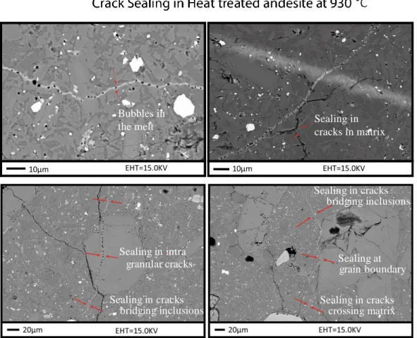
with the presence of a small fraction of clay (3%) in the intact andesite. Indeed, for heat
treatment above 500°C, some clay melting is observed and contributes to sealing the longest
cracks.
Secondly, we present samples artificially altered at different levels after heat-treatment. We
report results of hydrostatic and triaxial loading experiments performed on untreated, unaltered
heat-treated and artificially altered samples, all originally from the exact same lithology. The
evolution of the mineralogy with both the heat treatment and the artificial alteration was
heat treated andesite. The weakening is stronger as alteration is higher. (3) Smectite is observed
to precipitate in cracks in artificially altered samples. (4) A decrease of the friction coefficient
in cracks due to the presence of smectite might explain the mechanical weakening of altered
sample.
At last, a series of experiments were performed in order to investigate the effect of fluid
pressure variation i) on the mechanical behavior of andesite samples and ii) on acoustic
emissions activities. Fluid pressure was raised in a sample submitted to a stress state close to
the onset of dilatancy (which corresponds to the critical stress state in field), and the injection
was continued until the rupture (the axial stress and confining pressure were kept constant).
Fault propagation was monitored by the acoustic emissions. Our results show that (1) A time
dependent behavior was observed in the fluid-injection induced rupture experiment. (2) Spatial
heterogeneity of crack development was observed before rupture. More cracks were developed
at downstream while upstream remains silent and the rupture began from the downstream end.
(3) Critical crack length is inverted and estimated to be in the range of 129μm~223μm. Finally,
in a second series of experiments, we employed optic fiber sensors to measure the fluid pressure
at different positions in the sample during the pressure diffusion process. Axial strain and radial
strain were recorded during the whole process. After experiment, CT-scan was performed on
the sample after fluid injection experiment to observe the fractures network. Our results show
that (1) permeability heterogeneity is observed during the fluid-injection experiment. (2)
Subcritical crack growth influences the permeability and pore pressure spatial temporal
distribution.
Résumé
Comprendre et connaitre les propriétés physiques et le comportement mécanique de l'andésite
est important pour des applications industrielles comme la géothermie ou le stockage de CO2
mais aussi pour comprendre différents processus naturels.
Dans une première partie, on étudie l’effet des fissures d’origine thermique sur les propriétés physiques et les processus de rupture de l'andésite. Le comportement mécanique est étudié via
des tests triaxiaux à taux de déformation constante et à température ambiante. La fissuration
thermique a été induite en chauffant et en refroidissant lentement des échantillons. Les effets
de des traitements thermiques pour des amplitudes comprises entre 500 ° C et 1100 ° C sur la
vitesse des ondes P et sur la microstructure ont été étudiés. Ensuite, les propriétés mécaniques
des échantillons d'andésite traités à 930 ° C ont été étudiées sous contrainte triaxiale et à
température ambiante en utilisant des tests à taux de déformation constant et à des pressions de
confinement comprises entre 0 et 30 MPa. Nos résultats montrent que 1) pour les traitements
thermiques inférieures à 500 ° C, aucun changement significatif des propriétés physiques n’est observé; 2) pour les traitements thermiques dans la plage de températures de 500-1100 ° C, la
densité de fissures augmente; et 3) la fissuration thermique n'a pas d'influence sur l'apparition
de la dilatance mais augmente la résistance mécanique des échantillons traités thermiquement.
La présence d'une petite fraction d'argile (3%) dans l'andésite intacte peut expliquer ce résultat.
En effet, pour les traitements thermiques supérieurs à 500°C, une partie de l'argile fond et
colmate les fissures les plus longues.
Deuxièmement, nous avons effectué des recherches sur les effets de l'altération sur le
comportement mécanique et sur la minéralogie. Nos résultats montrent que (1) les modules élastiques de l’andésite altéré au laboratoire augmentent en fonction du degré d’altération. (2)
L'affaiblissement est d'autant plus fort que l'altération est élevée. (3) On observe que la smectite
précipite dans les fissures pour les échantillons altérés au laboratoire. (4) Une diminution du
coefficient de frottement dans les fissures en raison de la présence de smectite pourrait
expliquer l'affaiblissement mécanique de l'échantillon altéré.
Enfin, une série d'expériences a été réalisée afin d'étudier l'effet de la variation de la pression
du fluide i) sur le comportement mécanique des échantillons d'andésite et ii) sur les activités
d'émissions acoustiques.. La pression du fluide a été augmentée dans un échantillon soumis à
un état de contrainte proche du seuil de dilatance (ce qui correspond à l'état de contrainte
critique sur le terrain), et l'injection a été poursuivie jusqu'à la rupture (la contrainte axiale et
la pression de confinement ont été maintenues constantes). Nos résultats montrent qu’un (1)
comportement dépendant du temps est observé dans l'expérience de rupture induite par
injection de fluide. (2) Une hétérogénéité spatiale du développement de la fissuration est
observée avant la rupture. (3) La longueur critiques des fissures est inversée et estimée entre
129 µm et 223 µm. Dans une seconde série d’expérience, nous avons utilisé des capteurs à fibres optiques pour mesurer la pression du fluide à différentes positions de l'échantillon
pendant le processus de diffusion de la pression. Après l'expérience, un scanner a été réalisé sur l'échantillon pour observer le réseau de fractures. Nos résultats montrent qu’(1) une hétérogénéité spatiale de la perméabilité est observée au cours de l'expérience d'injection de
fluide. (2) La croissance de la fissure sous-critique influence la perméabilité et la distribution
spatio-temporelle de la pression interstitielle.
Acknowledgement
I am deeply grateful for my three supervisors: Dr. Jerome Fortin, Prof. Yves Gueguen, Prof.
Chunhe Yang for their support and patience at all times. Jerome is always happy, optimistic,
and with a lot of ideas, he gives me a lot of confidence and valuable advices in the long
uncertain research process. It has been a pleasure to work with him. He helped and supported
me so much both in academic and in life that I can finish my PhD smoothly in a foreign country.
Yves is like a big detective, he provided visions and philosophical concepts in research, and he
is always patient with young researchers. He is a real gentleman and I learned more from him
except from research. I give my deep gratitude to Prof. Yang who supported me a lot and gave
me opportunity to go abroad.
I would like to thank Dr. Aurelien Nicolas who has given me a lot of help on doing experiments
and processing data, and discussion during my PhD. Many thanks to Lea levy, Sissmann,
Cedric Bailly, Jan Borgomano, Chao Sun for their help on microstructure analysis and model
construction. I wish to thank Dr. G. Blocher, C.Kluge, and Dr. H. Milsch in GFZ for their kind
help in the experiments and discussion. I express my gratitude to Prof. Chopin, Dr. Thomas
Ferrand and Dr. Sarah Incel for their discussion with me, and Damien Deldicque for his help
in SEM and XRD analysis. My special thanks to Fredric Pellet and Dominique Bruel for
attending my committee during my PhD.
I would like to thank Mr. Stephane Richard and Mr. Phillipe who helped me a lot in the
administrative procedures and visa issues. I’m sincerely grateful for Laure Meynadier, Helene
Lyon-caen, and Clement Narteau who have given me a lot of encouragement and teach me to
balance between life and academic.
Alexandre Schubnel, Christophe Vigny, Harsha Bhat, Manuel Pubellier, Matthias Delescluse,
Matio, Romain Jolivet, Luce Fleitout and Cedric Bulois. Deep thanks to my dear friends,
Paoline Prevost, Eva Kanari, Sungping Chang, Hanjn Yin, Gianina,Valentin Tschannen,
Lavynia Tunini, Chao Sun, Louise Cordrie, Samanul Chapman, Yao Liang, JB, JD, Manon
Dlsn, Kurama Okubo, DJ, Juan Martin de Blas, Thomas Chartier, Arefeh Mrf, Amin Kahrizi,
Menglan He, Wei Wei, Ying Zhu, Yue Jiang, Alice Wang, Zhikai Wang, Zhiyi Qiu, Zhi Geng,
Jialan Wang, Yijing Wu, Jingjing Lu, Guanglei Cui, Qi He, Jingtian Xu, Xiaoping Yuan, Lei
Wang, Zhenkun Hou, Shuai Heng, Yunlong Wei, Mingjie Gao. My special thanks to my
landlady Madame Chiffert and Mr. Olivier Chiffert, and Sichelle Chiffert.
This research is sponsored by China Scholarship Council and GEOTREF France, my special
thanks to them and to ENS and ISRM, Chinese Academy of Sciences, which gave me the
chance to do PhD.
I wish to greatly appreciate the help and support of Dr. Fei Zheng for being with me at best
times and worst times.
At last to my beloved family, I am deeply grateful that my younger brother and my parents are
Table of Contents
Abstract ... I
Résumé ... III
Acknowledgement ... V
Table of Contents ... VII
Introduction ... 1
Research background ... 1
Scientific problems addressed in this thesis... 2
Geodynamic setting: La Guadeloupe ... 4
Research Outline ... 7
Chapter Ⅰ Methodology and Theoretical Background ... 10
1.1 Methodology ... 10
1.1.1 Experiment apparatus... 10
1.1.2 Strain and ultrasonic measurements ... 10
1.1.3 The brittle regime: definition of the stress states C’ and D’ ... 13
1.1.4 Ultrasonic measurements and acoustic emission (AE) ... 15
1.1.5 Velocity model for AE hypocenter location ... 16
1.1.6 Acoustic location algorithm ... 17
1.1.7 Permeability measurement ... 20
1.2.2 Effective Medium Theory ... 23
1.2.3 Wing crack model ... 27
1.2.4 Subcritical crack growth ... 30
1.2.5 Stress-dependent permeability ... 31
1.2.6 Construction of a nonlinear diffusion equation ... 31
Chapter Ⅱ Physical and Mechanical Properties of Thermally Cracked Andesite Under Pressure ... 34
2.1 Introduction ... 35
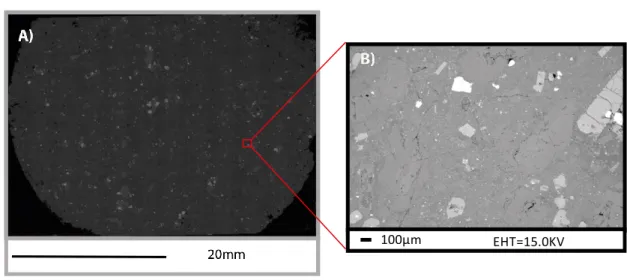
2.2 Material & Methods ... 37
2.2.1 Materials ... 37
2.2.2 Experimental Methods ... 39
2.3 Results ... 41
2.3.1 Properties of samples heat-treated at different temperatures ... 41
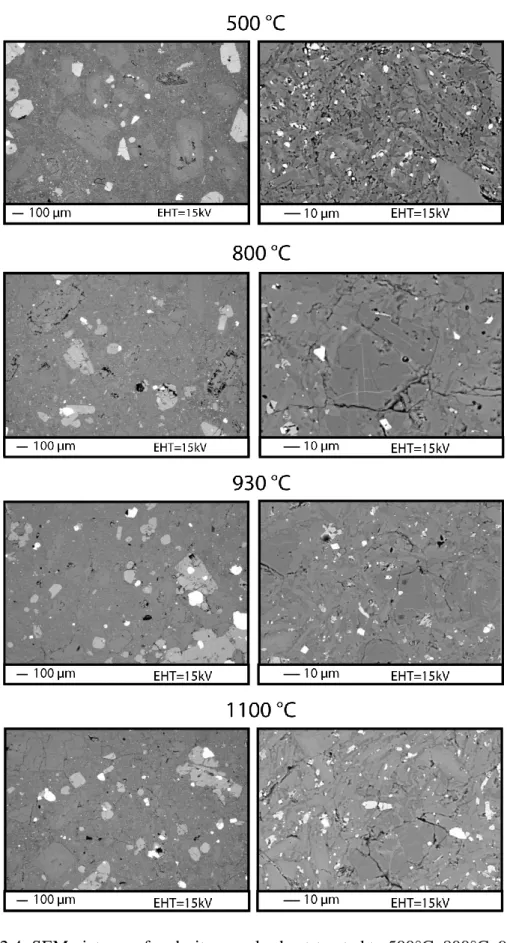
2.3.2 Mineralogical effects of heat treatment on andesite ... 45
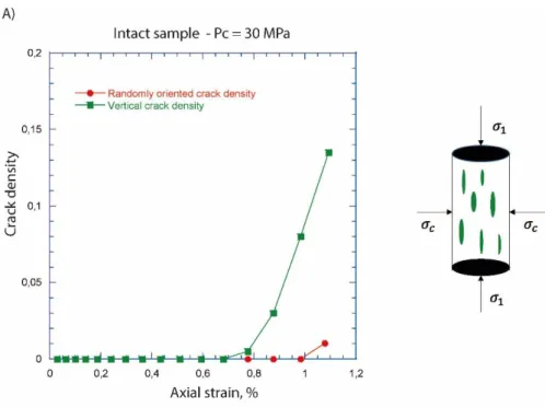
2.3.3 Tri-axial deformation of non-heat-treated andesite and heat-treated andesite ... 48
3.3.4 Ultrasonic velocity evolution of heat-treated andesite... 54
2.4 Discussion ... 56
2.4.1 Effect of the heat treatment on the crack density ... 56
2.4.2 Effect of heat treatment on the microstructure: partial melting ... 59
2.4.3 Effect of heat treatment on mechanical strength... 60
Chapter Ⅲ Influence of Hydrothermal Alteration on The Elastic Behavior and Failure
of Heat-Treated Andesite from Guadeloupe ... 69
3.1 Introduction ... 70
3.2 Material and methods ... 71
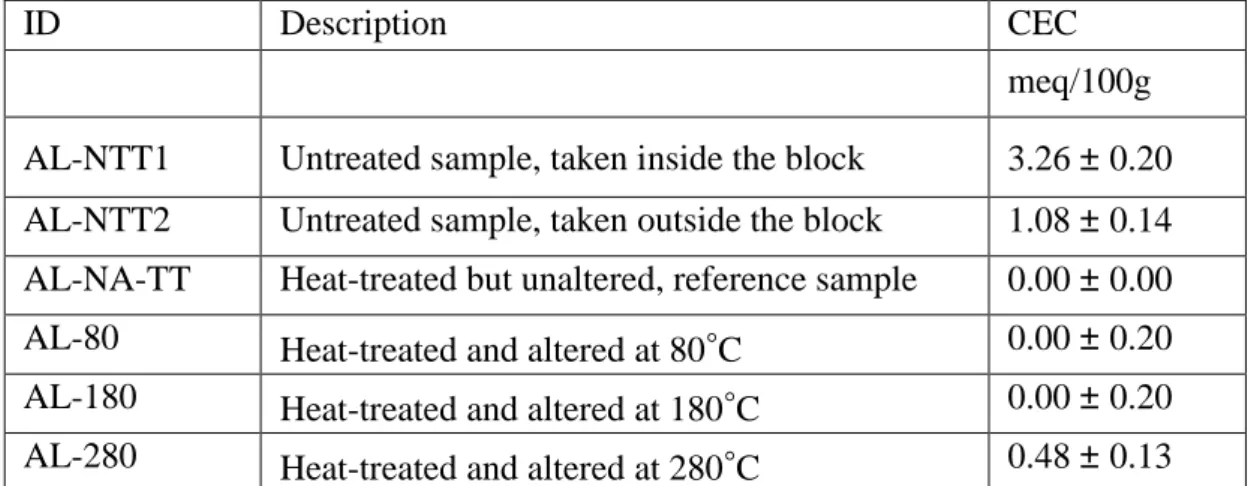
3.2.1 Starting material, heat-treatment and artificial alteration ... 71
3.2.2 Characterization of mineral sand chemical contents ... 72
3.2.3 Petrophysical properties ... 73
3.2.4 Experimental Apparatus ... 74
3.3 Results ... 75
3.3.1 Evolution of mineralogy with heat-treatment and alteration ... 75
3.3.2 Evolution of petrophysical properties with heat-treatment and alteration ... 81
3.3.3 Evolution of the elastic behaviour under hydrostatic stress with heat-treatment and alteration ... 82
3.3.4 Evolution of the mechanical behaviour during triaxial loading and failure with heat-treatment and alteration... 85
3.4 Discussion ... 91
3.4.1 Alteration, porosity and density ... 91
3.4.2 Can smectite precipitation in cracks explain the mechanical behaviour? ... 91
3.4.3 Modelisation ... 93
3.4.4 Implications... 96
Chapter Ⅳ Fluid-Injection Induced Rupture in Thermally Cracked Andesite at
Laboratory Scale ... 99
4.1 Introduction ... 100
4.2 Material & Methods ... 102
4.2.1 Materials ... 102
4.2.2 Experiment Methods ... 104
4.3. Results ... 105
4.3.1 Mechanical properties of heat-treated andesite under hydrostatic loading ... 105
4.3.2 Differential loading of heat-treated andesite sample under saturated condition. .. 108
4.3.3 Fluid injection induced rupture on heat-treated andesite sample ... 111
4.4 Discussion ... 124
4.4.1 Crack density inverted from hydrostatic loading under dry condition ... 124
4.4.2 Aspect ratio/crack length/crack aperture inverted from hydro-loading under saturated conditions ... 125
4.4.3 Fluid injection into heat treated saturated andesite sample ... 126
4. 5 Conclusions ... 130
Chapter Ⅴ Permeability Evolution and Its Effect on Fluid Pressure Temporal Spatial Distribution during Fluid Injection ... 132
5.1 Introduction ... 132
5.2 Methodology ... 134
5.2.1 Sample preparation ... 134
5.2.3 Optical Fibers ... 136
5.3 Results ... 140
5.3.1 Fluid pressure temporal spatial distribution ... 140
5.3.2 Permeability variation space & time ... 142
5.3.3 A clear heterogeneity of crack development (CT images) ... 143
5.4 Discussion ... 144
5.4.1 boundary condition ... 145
5.4.2 Equation setup ... 145
5.4.3 Solution of pore pressure at different positions and time ... 146
5.5 Conclusions ... 149 Conclusions ... 150 References ... 152 Chapter I References ... 152 Chapter Ⅱ References... 158 Chapter Ⅲ References ... 164 Chapter Ⅳ References ... 173 Chapter Ⅴ References ... 178
Introduction
Research background
In geothermal systems, the physical properties and mechanical behavior of andesite are of
interest for the understanding of several natural processes and for engineering design. Natural
processes include ground deformation due to magma rising below volcanoes (Jaupart,1998;
Costa et al. 2009; Heap et al.2014), eruption activity and formation of dikes (Gudmundsson,
2006,2011; Browning et al. 2015), or fault activity (Rowland and Sibson, 2001). Industrial
contexts are geothermal reservoir engineering (Siratovich et al., 2014) and CO2 sequestration
(Trias et al. 2017).
As geothermal fields usually locate in tectonically active areas, crustal stresses are near to
critical stress. In addition, tectonically active areas mean “fractured rock reservoir”. Several
authors have investigated the effect of micro-fracture on mechanical strength, porosity, elastic
wave velocities, and elastic moduli of rocks (Wu et al. 2000; Guéguen and Schubnel 2003;
Smith et al. 2009, Pereira and Arson 2013; Faoro et al. 2013; Pola et al. 2014; Heap et al. 2014).
The link between micro-fractures and permeability (Nara et al. 2011) has been also investigated,
with micro-fractures proving to enhance permeability.
Fluid pressure variation has influence on different aspects of geothermal systems. Fluid
pressure variation can be associated with seismicity observed in natural processes such as
seasonality of ground water recharge (Hainzl et al. 2006; Saar and Manga, 2003), water level
fluctuations in water reservoirs (Chander, 1997; Talwani 1997), petroleum exploration (Davies
et al., 2013; Rutqvist et al., 2013) , geothermal field (Baisch et al., 2010; Deichmann and
Giardini, 2009; Brodsky et al., 2000; Prejean et al. ,2004; Giardini 2009), wastewater disposal
(Zoback and Gorelick, 2012; Mazzoldi et al., 2012; Cappa and Rutqvist, 2011). Note that fluid
pressure variation could trigger earthquake (Yamashita 1998; El Hariri et al., 2010) in long
space and time scales (Hummel and Müller, 2009; Shapiro et al., 1997, 2003;).
Scientific problems addressed in this thesis
1. Thermal effect on mechanical properties of geothermal/volcano systems
In volcanic areas, where hot fluids circulate, temperature is a parameter that should be taken
into account when investigating mechanical behavior. Temperature variations can induce
intragranular cracks and intergranular cracks or even melting of the rock (Friedman et al. 1979,
Wong 1989), leading to large changes in the microstructure.
Many studies have been performed on the role of thermal effects on the mechanical behavior
of igneous rocks, including intrusive and extrusive rocks (Heap et al. 2014, 2015, 2016;
Vinciguerra et al. 2005; Fortin et al.2011; Stanchits et al. 2006; Meredith et al. 2005; Wang et
al. 2013). Note that, in contrast to intrusive rocks, extrusive rocks have a different
microstructure resulting from fast cooling: a fine groundmass and phenocrysts.
Increasing temperature can modify fluid transport properties (Vinciguerra et al. 2005, Nasseri
2009, Faoro, 2013, Darot, 1992, Geraud 1994), elastic wave velocities (Walsh 1965, Nasseri
2007), and mechanical properties (Faulkner et al. 2003, Wang et al. 2013). Thermal cracking
has been shown to weaken different rocks, including granite (Homand-Etienne and Houpert,
1989; Chaki et al. 2008), gabbro (Keshavarz et al. 2010), calcarenite (Brotóns et al. 2013), and
carbonate (Sengun et al. 2014;). P-wave velocity changes due to thermal cracking are expected.
Such changes are important for seismic tomography inversion of volcano systems and may be
useful for investigating magma chamber activity and dike eruption. Because induced seismicity
geo-2. Hydro-thermal effect of alteration on the properties of geothermal system
In volcanic geothermal systems [e.g. Reyes, 1990; Meunier, 2005], subduction zones [e.g.
Hyndman et al., 1997;Passellegue et al., 2014] and some major faults [e.g. Chester et al., 2013;
Yamaguchi et al., 2011], where hot fluid circulates in the host rock [e.g. Adelinet et al., 2011],
the presence of alteration minerals is susceptible to significantly modify the mechanical
behaviour of rock, as compared to pure and healthy rock. Alteration results in microstructural
changes [e.g. Heap et al., 2014; Siratovich et al., 2014], which in turn modifies the physical
(porosity, open crack density, velocity of propagation of elastic waves, permeability) and
mechanical properties of the rock [Pola et al., 2012; Meller and Kohl, 2014; Frolova et al.,
2014; Wyering et al., 2014]. Small changes in microstructural parameters, such as porosity [e.g.
Vajdova et al., 2004], pore size [e.g. Zhu et al., 2010], crack density and mean length [e.g.
Keshavarz et al., 2010], significantly affect the mechanical behavior of volcanic rocks.
3. Fluid pressure variation induced seismicity
The potential risk of inducing seismicity by diffusion of elevated pore pressure is known for
decades (Ellsworth 2013). In addition, since 2008, fluid injection used for shale gas production
appears to be the trigger of earthquakes in the mid-continent of United States which has become
seismically active (Frohlich et al. 2012,2013,2014; Horton 2012; Keranen et al. 2013;
Ellsworth 2013; Justinic et al. 2013; McGarr et al. 2014,2017). As an example, a magnitude of
4.8 earthquake occurred near Timpson, Texas, a region where the seismicity was rare prior to
this earthquake event (Frohlich et al, 2014). In Europe, the Deep Heat Mining Project in Basel,
Switzerland used fluid injection to increase the permeability of the reservoir (fractures in
granite) and caused a event with a magnitude of 3.4 (Giardini 2009, McGarr et al. 2014,2017).
Geothermal systems are commonly hosted in altered and fractured rock reservoir (Wu et al.
geothermal fields usually locate in tectonically active areas, crustal stresses are near to critical
stress (Ellsworth 2013; Zoback et al. 1997), thus fluid injection in these reservoirs could induce
seismicity.
At field scale, time lag effect of induced seismicity due to fluid injection has been observed.
Shirazi et al. (2016) used INSAR data to estimate pore pressure and volumetric strain. As soon
as the injection is stopped, the authors show that the pore pressure has an inhomogeneous
spatial distribution: the areas with high permeability are associated with the largest pore
pressure decay, whereas the areas associated with low permeability are associated with high
fluid pressure.
4. Spatiotemporal pattern of seismicity related to hydraulic diffusion
Different hydraulic diffusivity and seismic criticality (mechanical property) of rocks lead to
different spatiotemporal pattern of seismicity activity (Do Nascimento et al., 2005; Shapiro et
al., 1997, 2003). Hummel and Müller, (2009) included the permeability change in the model of the fluid pressure diffusion. Yilmaz et al. (1994) investigated pore fluid pressure distribution
in fractured and compliant rocks by simulating 1-D pore-fluid pressure profiles with a
pressure-dependent permeability. Pore pressure propagation is highly influenced by the permeability
heterogeneity of the crust (Lee et al., 1998; Clifton et al., 2003; Do Nascimento et al., 2005;).
It’s important to account for geologic complexity when estimate the transmission of pore poressre while investigate seismicity (Simpson and Narasimhan, 1992; Lee et al., 1998; Do
Nascimento et al., 2005).
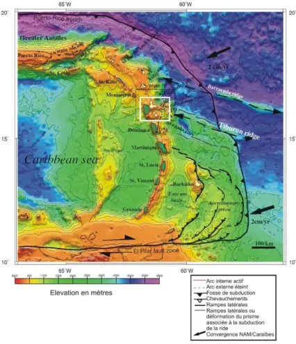
Geodynamic setting: La Guadeloupe
long between the island of Saba in the North and Grenade in the South. Most of the magmatic
products found in the island arc are related to the subduction of the North American Plate below
the Carribean plate since at least 40 Ma (Bouysse et al., 1990). Being part of the northern part
of the arc, Guadeloupe displays both the recent active volcanic arc and the old extinct arc
(Bouchot et al., 2011).
Figure 1. Geodynamical map of the Lesser Antilles showing the old extinct arc (dotted
redline) and the recent active are (plain red line). Guadeloupe Archipelago is showed within
the white box. (Feuillet et al., 2001; Bouchot et al., 2011).
Regional seismicity affecting Guadeloupe is related to the oblique subduction of the North
American plate below the Caribbean plate as well as to movements along normal faults and
has been responsible for damaging shallow-depth M ≥5 earthquakes in 1851 and 1897.
earthquakes are related to the volcanic complex (La Soufrière) formed at the western tip of a
prominent E-W oriented graben, whose normal faults extend from the prominent
Marie-Galante rift system.
Basse Terre is a volcanically active island located in the central part of the Lesser Antilles
volcanic arc. The northern part of the island is made of the NNW–SSE-elongated Northern
Chain. This part of the island is the oldest one (Davidson et al., 1983; Bouysse et al.,1990;
Samper 2008;), and is formed from high eruption rates and/or low viscosity magma that
propagated within extensional structures parallel to the volcanic front. The morphology of this
island has been substantially modified by erosion. The southern part of the island (the youngest
part) is made of volcanoes with more circular bases, formed by lower eruption rates and/or
more viscous magma that exploited the NW–SE-striking Montserrat-Bouillante fault zone.
Sample material
GEOTREF (A project aimed at improving understanding fractured geothermal reservoirs) is
planning a new geothermal project in the area from which the samples were taken. For the
purpose of our research we selected six andesitic blocks from different areas in La Guadeloupe.
Two blocks are from the quarry of Deshaio are used for the research in this thesis.
Note that the temperature of 930°C that we will used in the next chapter, for the amplitude of
the heat-treatment, corresponds to the temperature of the second magma chamber in La
Soufière (Villemant et al. 2014), which is where the dikes begin (Villemant 2014).
Figure 3. Villemant et al., 2014
Research Outline
Chapter I gives a review on methodology and theoretical background. The experimental set-up
of the tri-axial cell, strain measurements, hardware and software of acoustic survey system are
described. Theoretical models employed in this research are reviewed, including effective
medium theory, fracture mechanics, wing crack model, subcritical crack growth, nonlinear
diffusion equation.
Chapter II presents the effects of thermal crack damage on the physical and mechanical
properties of an andesite. Thermal cracking was induced by slowly heating and cooling
samples. The effect of the temperature of the heat-treatment ranging between 500 °C and
mechanical properties of andesite samples treated to 930 °C were investigated under triaxial
stress at room temperature, using constant strain rate tests and at confining pressure ranging
between 0 and 30 MPa. Similar triaxial experiments were conducted on non-heat-treated
samples. This chapter has led to a paper under press in Rock Mechanics and Rock Engineering.
Chapter III presents samples artificially altered at different levels after heat-treatment. We
report results of hydrostatic and triaxial loading experiments performed on untreated, unaltered
heat-treated and artificially altered samples, all originally from the exact same lithology.
During these experiments, evolution of P- and S wave velocities were measured to track the
evolution of cracking. Acoustic emissions were also recorded and localized. The evolution of
the mineralogy with both the heat treatment and the artificial alteration was also carefully
tracked, with a special focus on smectite and other clay minerals precipitation. This chapter has
led to a paper that will be submitted soon.
Chapter IV shows a series of experiments done in order to investigate the effect of fluid
pressure variation i) on the mechanical behavior of andesite samples and ii) on acoustic
emissions activities. In particular fluid pressure was raised in a sample submitted to a stress
state close to the onset of dilatant point (corresponds to the critical stress state in field), and the
injection was continued until the rupture (the axial stress and confining pressure were kept
constant). Fault propagation were monitored by the acoustic emissions, and their locations were
compared with the fractures observed in the sample after the experiment. The mechanism of
delayed time before the main rupture is discussed.
Chapter V investigates the fluid pressure diffusion in rock submitted to stresses closed to the
criticality. We performed a fluid injection experiment on the thermally treated andesite and
monitored pore pressure in a space-time domain. Firstly, hydrostatic loading is applied on the
constant value (35 MPa), until the whole sample reaches failure. We employed optic fiber
sensors to measure the fluid pressure at different positions of the sample during the pressure
diffusion process, axial strain and radial strain are recorded during the whole process. After
experiment, CT-scan was performed on the sample after fluid injection experiment to observe
Chapter Ⅰ Methodology and Theoretical Background
1.1 Methodology
1.1.1 Experiment apparatus
Experiments were performed using a tri-axial cell installed in Laboratoire de Geologie at Ecole
Normale Supérieure in Paris. This apparatus allows for hydrostatic and deviatoric loading, pore
pressure and temperature to be applied independently on a cylindrical specimen (diameter 40
mm length 80 mm). The hydrostatic and deviatoric stresses are servo-controlled with an
accuracy of 0.01 MPa, and oil is used to confine the whole sample within the cell. The pore
pressure, the confining pressure and the deviatoric stress can be increased respectively up to
100, 100 and 700 MPa. Temperature can be increased up to 200°C but only room temperature
data are reported in this work. Room temperature is controlled with an accuracy of ±0.5 C
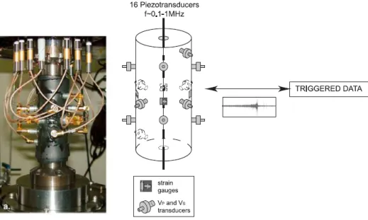
around 20°C. A schematic diagram of the setup is presented in Figure 1.1.
1.1.2 Strain and ultrasonic measurements
Eight Tokkyosokki TML FCB strain gages (four axial and four circumferential) were glued
directly onto the surface sample (Figure 1.2). Each strain gauge is used in conjunction with a
one-fourth Wheatstone bridge. The strain measurement is recorded every two seconds. An
external gap sensor using Foucault currents is employed to measure the total displacement of
the piston during axial loading and provides, once corrected, a global axial strain measurement.
The measured axial strain 𝜀1 and radial strain 𝜀3 allow for the estimation of the volumetric
strain 𝜀𝑣 = 𝜀1+ 2𝜀3 and the calculation of the static Young modulus. Axial strain 𝜀1 and radial
and the four horizontally oriented strain gauges, respectively. The compressive stresses and
strains are denoted as positive.
Figure 1.1 Tri-axial cell installed at École Normale Supérieure (Ougier-simonin et al., 2010, 2011)
Figure 1.2 Ultrasonic sensors and strain gauges glued on samples (from Ougier-Simonin et
1.1.3 The brittle regime: definition of the stress states C’ and D’
The failure of brittle rocks has been investigated by many researchers (Brace et al.,1966;
Bieniawski, 1967; Byerlee and Brace, 1968; Scholz, 1968; Wawersik and Fairhurst, 1970;
Martin and Chandler, 1994; Wong et al., 1997). They have shown that the stress-strain curves
for a brittle material can be divided into five regions (Figure 1.3) (Martin and Chandler 1994).
The initial region of the stress-strain curve represents the closure of existing micro-cracks in
the sample and may or may not be present, depending on the initial crack density and crack
geometry (Martin and Chandler 1994).
Once the existing cracks are closed, the strain-stress curve is usually linear (Figure 1.3 - region
II). The elastic properties could be determined from this part of stress-strain curves.
The onset of dilation marks the beginning of region III. Brace et al. (1966) found that dilation
begins at a stress level of about 40-60% of the peak strength. This stress level is referred to as
the crack initiation stress 𝜎𝑐 (C’ point). These cracks are stable cracks since an increase in load
is required to cause further cracking. Crack initiation is difficult to identify from the laboratory
stress-strain curves, particularly if the sample already contains a high density of micro-cracks
(Martin and Chandler, 1994; Wong et al., 1997; Brace et al., 1966; Scholz, 1968; Baud et al.
2000; Richart et al. 1928). The crack initiation stress is best determined using a plot of
volumetric strain versus axial strain (figure 1.3). First the elastic volumetric strains are
calculated using the elastic constants (𝐸, 𝜐) from the linear portion of stress-strain curves in
region II by
∆𝑉 𝑉𝑒𝑙𝑎𝑠𝑡𝑖𝑐=
1−2𝜐
𝐸 (𝜎1− 𝜎3) ,
Then, the elastic volume strain are subtracted from the total measured volumetric strains to
Figure 1.3 Martin and Christiansson, 2009
The axial stress level 𝜎𝐷 (D’ point) where the total volumetric strain reverse from compaction
to dilatancy marks the beginning of region IV (Figure 1.3) and represents the onset of unstable
crack growth, as defined by Bienawaski (1967). It generally occurs at axial stress level between
70%-90% of the short-term peak strength. It is at this stress level that the axial strain departs
from linearity (figure 1.3). Hallbauer et al. (1973) pointed out that this region is characterized
by the most significant structural changes to the sample, with the density of micro-cracks
increasing drastically.
The peak strength of the material marks the beginning of post-peak behavior, Region V, and is I II III IV V C’ I II III IV V D’ D’ C’
1.1.4 Ultrasonic measurements and acoustic emission (AE)
14 ultrasonic piezoelectric transducers (PZTS, Figure 1.2) were glued directly on the surface
of the sample. The classical ultrasonic pulse transmission technique is used for velocity
measurements between an emitting and a receiving transducer (Ougier-Simonin et al., 2011).
It consists of measuring the travel time of an elastic pulse through the rock sample for a known
travelling path length, the latter having been corrected for strains during the mechanical loading.
In active velocity survey mode, a pulse of 250 V with a rise time of 1s is generated and
transmitted successively to each transducer using a pulsing switchbox (ASC Ltd.). Each
piezo-ceramic converts this electrical pulse into a mechanical vibration that propagates into the
medium. In contrast, each receiving piezoceramic converts the received mechanical waveform
into an electrical signal that is amplified at 40 dB using 16 pre-amplifiers. Signals are recorded
using a 16 channels Cecchi digital oscilloscope. Waveforms are sampled at 50MHz. Velocity
surveys were then fully automatically processed using cross-correlation techniques so that the
error bar on wave velocity measurements are less than 2%. This specific arrangement permitted
measurements of P-wave anisotropy in our sample throughout experiment. These
measurements allowed us to identify the dynamic elastic constants.
In passive mode, each transducer signal is recorded using the ASC Ltd. MiniRichter streaming
system, which stores continuous ultrasonic waveform data onto a 1 TB hard disk (Figure 1.2).
Such continuous recording techniques at this sampling rate have been pioneered in the last
years thanks to fast development of computing systems. Signals were amplified at 40 dB as
well. In these conditions, the average electric noise was kept below 15 mV on most channels.
Discrete acoustic emissions data was obtained after the experiment using a simple triggering
technique (300 mV minimum amplitude, 5 ls time window) on waveform records. Time of the
Hypocenter locations were then determined using a collapsing grid search algorithm, assuming
an evolutive medium (from isotropy to transverse isotropy using the velocity model calculated
in active mode). The AE hypocenter location was used to determine the origin of the acoustic
signals generated during fracturing.
1.1.5 Velocity model for AE hypocenter location
(1) Homogeneous isotropic
The homogeneous isotropic velocity structure assumes a half space containing the source and
all receivers. Each raypath is calculated as a vector between the source and the receiver.
Velocity is homogeneous throughout the volume and isotropic. For isotropic symmetry, the
relation of elastic velocity and shear modulus 𝐺, bulk modulus 𝐾
𝑉𝑃 = ( 𝐾 + 4𝐺/3 𝜌 ) 0.5 𝑉𝑠 = (𝐺 𝜌) 0.5 (1-1) (1-2) (2) Transversely isotropic
For transversely isotropic velocity structure, velocity varies depending on the ray orientation
through the volume with respect to an axis of symmetry. The direction of axis is defined by a
vector a, in a North-East-Down Cartesian coordinate system using an azimuth from North and
plunge down from the horizontal (Insite Appendices). The velocity (P or S wave velocity) is
given by equation 3-1 where 𝛾 is the angle between the raypath 𝑙 and the axis of symmetry a.
𝑉𝐼 is the velocity parallel to the axis of symmetry, 𝑉− is the velocity perpendicular to the axis
Where α is the anisotropy factor. The velocity 𝑉𝑟 along the raypath 𝑙 is (Insite Appendices)
𝑉𝑟 = (𝑉𝐼+ 𝑉−
2 ) − (
𝑉𝐼− 𝑉−
2 )cos (𝜋 − 2𝛾) (1-4)
1.1.6 Acoustic location algorithm
(1) Geiger routine
The Geiger algorithm solves for the origin time t0, and source location (x0, y0, z0), such that the
sum of the square of the residuals is a minimum, where the residual r is equal to the observed
time t0 minus the calculated time at (x0, y0, z0). The algorithm iterates towards the correct
location using the magnitudes of the time derivatives. The Geiger method is an inverse least
square problem. The source location is defined by four parameters:
𝜃 = (𝑡0, 𝑥0, 𝑦0, 𝑧0) (1-5)
The time residual 𝑟𝑖 is the difference between the calculated arrival times 𝑇𝑖 and the observed
arrival times 𝑡𝑖 corrected to the time zero of the event 𝑡0:
𝑟𝑖 = 𝑡𝑖 − 𝑡0− 𝑇𝑖 (1-6)
The function relating the arrival times and the location is nonlinear since there is no single step
approach to find the best event location. The standard technique is to linearize the problem:
𝜃 = 𝜃∗+ ∆𝜃 (1-7)
Where 𝜃∗ is a source location estimate near the true location, and ∆𝜃 is a small perturbation.
Using the first term in the Taylor series expansion, the observed times may be approximated
by
𝑡𝑖 = 𝑡0∗+ ∆𝑡0+ 𝑇𝑖(ℎ∗) +
𝜕𝑇𝑖
𝜕ℎ ∆ℎ (1-8)
𝑟𝑖(ℎ∗) = ∆𝑡 0+ 𝛿𝑇𝑖 𝛿ℎ ∆ℎ (1-9) 𝑟𝑖(ℎ∗) =𝛿𝑇𝑖 𝛿𝜃 ∆𝜃 (1-10)
In matrix notation, equations could be expressed as
𝑟 = 𝐴∆𝜃 (1-11)
Following Gibowicz and Kijko [1994], the minimization of the sum of the squared time
residuals can be given by
𝑏 = 𝐵∆𝜃 (1-12)
The Geiger location is found by choosing a starting location, solving the matrix problem
(Singular Value Decomposition) for ∆𝜃, and then iterating until this adjustment parameter
reaches a user set minimum.
(2) Collapsing grid search routine
The algorithm searches a 3D space defined for the minimum misfit between the measured
travel times picked for every receiver and the theoretical travel times from the ray path and
given velocity model.
A collapsed grid has a size (volume limits) and cell dimension defined by the previous grid,
the dimension of a collapsed cell is given by
𝐷𝑐𝑖+1=𝐷𝑐𝑖
𝑅 (1-13)
Where 𝐷𝑐𝑖 is the Cell Dimension of the previous grid and R is the Collapsing Ratio. The
starting grid defined by the user can have any cuboid volume, whereas collapsed grids are
𝐷𝑔𝑖+1= 𝑁𝐷𝑐𝑖+1 (1-14)
Where N is the average number of axial cells in the starting grid. The number of axial cells
along each direction (North, East, and Down) in the starting grid is 𝐷𝑥/𝐷𝑐1 and must always
be ≥ 10. The cubic collapsed grid is defined by the user-specified Collapsing Buffer (𝐵𝑐), as
shown in figure 1.4, where 𝐵𝑐 is the half width of the new grid measured in number of
uncollapsed cells. The new grid thus has a side length of 𝐷𝑔𝑖+1 = 2𝐵𝑐𝐷𝑐𝑖 centered on a given
position in the uncollapsed grid. Thus if 𝐵𝑐 = 1 then the new collapsed grid has a volume
consisting of 8 uncollapsed cells (2×2×2) centered on the given position. If 𝐵𝑐 = 2 then the
new collapsed grid consists of 64 uncollapsed cells (4×4×4) and so forth.
Figure 1.4 Definition of a collapsed grid volume (Insite Appendices)
The Collapsing Ratio, R defines the collapsed Cell Dimension with respect to the uncollapsed
cell using first equation. The ratio is defined by
𝑅 = 𝑁
2𝐵𝑐 (1-15)
Collapsing Ratio must have a value 𝑅 ≥ 2.0 to ensure effective and efficient collapsing.
Collapsing grid search routine is applied for AE location in this thesis, it is more efficient as
an initial coarse grid is first searched for minimum misfit position. The algorithms assume that
position, then the minima is this collapsed grid will be found and another grid will be generated.
The method continues until a specified resolution is obtained.
1.1.7 Permeability measurement
For our permeability measurement we used two methods: steady state and transient pulse. The
steady state technique uses either a constant flow or a constant pore pressure gradient provided
by two servo-controlled cylinders. Two symmetrical measures of permeability were performed
by switching the flow direction in the sample. Permeability was then inferred using Darcy’s law:
𝑄
𝑆 = −
𝑘∆𝑃
𝜂𝐿 (1-16)
Where Q is the fluid flow (m3s-1), S the sample area (m2), L the sample length (m), η the
dynamic viscosity of the pore fluid (Pa·S), ∆𝑃
𝐿 is the pore fluid pressure gradient (Pa). However,
this method can only measure a permeability 𝑘 ≥ 10−18m2.
Transient pulse is used when permeability is lower (< 10−18m2). The fluid pressure on one
side of the sample is instantaneously increased by ∆𝑃. This allows us to measure the fluid
diffusion through the sample. ∆𝑃 decays exponentially with time until equilibrium pressure is
reached in the sample. Assuming the system geometry is known, the permeability could be
computed from the time it takes for this transient pressure pulse to reach the equilibrium (Brace
et al. 1968). 𝑘 = 𝛼𝜂𝛽𝐿 𝑆( 1 1 𝑉𝐴 + 1 𝑉𝐵 ) (1-17) With 𝑃 − 𝑃 = ∆𝑃 𝑉𝐴 𝑒−𝛼𝑡 (1-18)
𝑉𝐴 and 𝑉𝐵(m3) are the two cylinders reservoir volumes of the pore pressure pump respectively
(including the volume of the connecting tubes). 𝑃𝐴 is the pressure applied to 𝑉𝐴 instaneously
and 𝑃𝑓 is the final equilibrium. 𝛽 is the isothermal compressibility coefficient of the pore fluid
(Pa-1). 𝛼 is the decay exponent. According to Bernabe (1987), this method can be partly
modified by fixing the fluid pressure of the second cylinder constant. Thus the decay of the
pressure transient occurs more rapidly and the equation above is simplified to equation.
𝑘 = 𝛼𝜂𝛽𝐿
𝑆𝑉𝑝𝑢𝑙𝑠𝑒 (1-19)
𝑉𝑝𝑢𝑙𝑠𝑒 is the total fluid volume. In this case, 𝑉𝑝𝑢𝑙𝑠𝑒 = 𝑉𝐴 or 𝑉𝑝𝑢𝑙𝑠𝑒 = 𝑉𝐵, depending on whether
the pressure increment is applied on the cylinder 𝑉𝐴 or 𝑉𝐵.
1.2 Theoretical background
1.2.1 Fracture mechanics
(1) Strain energy
All materials have defects originally, Griffith, (1921) proposed that the defects concentrate the
stress, which lead with increasing stress to the final failure. Inglis, (1913) calculated the stress
concentrations around elliptical holes, but the singularity of the solution at the crack tip leads
to infinite stress. Griffith, (1921) employed an energy balance concept: the strain energy per
unit volume in a thin plate of linear elastic material submitted to an axial load and contain a
crack of radius c is 𝑈𝑒 = 𝐸𝜀 2 2 = 𝜋𝜎2𝑐2 𝐸 (1-20)
𝐸 is Young’s modulus of the material, 𝑈𝑒 is strain energy, 𝜎 is the axial stress, 𝜀 is the axial
𝑈 = −𝜎
2
2𝐸𝜋𝑐
2 (1-21)
The surface energy S associated with a crack of radius 𝑐 is
𝑆 = 4𝛾𝑐 (1-22)
𝛾 is surface energy density. The total energy associated with the crack is then the sum of the
(positive) energy absorbed to create the new surfaces, plus the (negative) mechanical strain
energy released by allowing the regions near the crack flanks to become unloaded.
(2) Unstable crack growth
In the beginning, cracks grow only with stress increasing. As the cracks grow longer, the crack
length reaches the critical crack length 𝑙𝑐, for which the crack growth is spontaneous and
catastrophic.
The critical crack length 𝑙𝑐 could be obtained by
𝜕(𝑆+𝑈) 𝜕𝑐 = 2𝛾 − 2 𝜎𝑓2 𝐸 𝜋𝑐=0 (1-23) 𝜎𝑓 = √ 𝐸𝛾 𝜋𝑐 (1-24)
𝜎𝑓 is the stress at failure. Irwin (1957) and Orawan (1949)suggested that in ductile materials
the released strain energy is absorbed not by creating new surfaces but by energy dissipation
due to plastic flow in the material near the crack tip. They suggested that the catastrophic
fracture occurs when the strain energy is released at a rate sufficient to satisfy the needs of all
these energy sinks. This critical strain energy release rate is denoted by the parameter 𝐺𝑐. The
Griffith equation can be rewritten in the form:
𝜎𝑓 = √𝐸𝐺𝑐
(3) Stress Intensity factor
Three types of cracks termed mode I, II and III are defined. Mode I is under tensile stress with
a normal-opening mode, while mode II and III are under shear stress with shear sliding modes.
Westergaard et al. (1939) gave the stress distribution at crack tip with stress intensity factors.𝐾𝐼,
𝐾𝐼𝐼, 𝐾𝐼𝐼𝐼 are stress intensity factor for mode I, II, III fractures respectively. The critical stress
intensity factor indicates the point where the material can withstand crack tip stresses up to a
critical value.
In plane stress condition for mode I:
𝜎𝑓= √ 𝐸𝐺𝑐 2𝜋𝑐= 𝐾𝐼𝑐 √2𝜋𝑐 (1-26) 𝐾𝐼𝑐2 = 𝐸𝐺 𝑐 (1-27)
where 𝐺𝑐 is the critical strain energy release rate, 𝐾𝐼𝐶 is fracture toughness, 𝐸 is elastic
modulus. In plane strain condition,
𝐾𝐼𝐶2 = 𝐸𝐺𝑐(1 − 𝜐2) (1-28)
1.2.2 Effective Medium Theory
(1) Definition of crack density and aspect ratio
When defects sizes are smaller than the wavelength, effective medium theory is an appropriate
method (Guéguen & Kachanov 2011).
The crack density 𝜌𝑐 is defined as
𝜌𝑐 = 1 𝑉∑ 𝑐𝑖 3 𝑁 1 (1-29)
Where 𝑐𝑖 is the radius of the i-th crack, N is the number of cracks in the Representative
Elementary Volume V.
The crack geometry is assumed to be penny-shaped (Bristow, 1960) and is indicated by average
aspect ratio:
𝜁 = 𝑤/𝑐 (1-30)
Where, 𝑤 is the half aperture of the crack, 𝑐 is the radius of the crack.
(2) Crack closure pressure
Defects in geo-materials are mainly cracks and pores. Aspect ratio of pores is close to 1 while
cracks have aspect ratio values < 0.01. Although cracks contribute little to porosity (<1%),
cracks dominate the effective properties of rocks (Simmons and Brace, 1965; Walsh, 1965a,
1965b; Brace et al., 1968; Gueguen et al., 2011).The closure pressure 𝑃𝑐𝑙𝑜𝑠𝑒 of cracks under
hydrostatic pressure in dry condition is (Walsh, 1965a; Jaeger et al., 2007):
𝑃𝑐𝑙𝑜𝑠𝑒 = 𝜋𝜁𝐸0
4(1 − 𝜐02)~𝜁0𝐸0 (1-31)
where, 𝐸0 and 𝜐0 are the Young modulus (GPa) and Poisson’s ratio of matrix, 𝜁0 is the initial
mean crack aspect ratio. Assuming for andesite 𝐸0 = 70 GPa, for pores 𝜁0 = 1 and crack
𝜁0=0.001, the closure pressure for pores are too high while for cracks the closure pressure is
70MPa approximately, showing a well know result that pores are stiffer to deform compared
to cracks.
(3) Non-interactive assumption in effective medium theory
The simplest method of all Effective Medium Theory is the non-interactive theory (Kachanov
effective medium theory was shown to be valid when cracks are distributed randomly and as
long as crack density do not exceed 0.3 (Kachanov, 1994; Sayers and Kachanov, 1995;
Schubnel and Gueguen, 2003; Fortin et al., 2006, 2007; Gueguen and Sarout, 2009). As a
consequence, crack density and mean aspect ratio could be inverted directly from elastic wave
velocities.
(4) Non-interactive assumption for randomly oriented cracks (including fluid effect)
In the framework of non-interaction approximation, the relation between elastic property
parameters and micro-structure parameters could be linked by (Bristow, 1960; Walsh 1965;
Fortin et al. 2006) 𝐾𝑜 𝐾 = 1 + 𝜌𝑐 ℎ 1 − 2𝜐𝑜 (1 −𝜐𝑜 2) (1-32) 𝐺𝑜 𝐺 = 1 + 𝜌𝑐 ℎ 1 + 𝜐𝑜(1 − 𝜐𝑜 5) (1-33)
𝐾 and 𝐺 are the effective bulk modulus and effective shear modulus respectively, which can
be inverted from ultrasonic velocities. 𝐾𝑜 and 𝐺𝑜 are the bulk modulus and shear modulus of
the crack-free matrix, 𝜐𝑜 is the Poisson ratio of the matrix, h is a factor given by
ℎ =16(1 − 𝜐𝑜
2)
9(1 −𝜐2𝑜) (1-34)
Under saturated condition, the equations are:
𝐾0 𝐾𝑠𝑎𝑡 = 1 + 𝜌𝑐 16(1 − 𝜐02) 9(1 − 2𝜐0)( 𝛿𝑓 1 + 𝛿𝑓) (1-35) 𝐺0 𝐺𝑠𝑎𝑡 = 1 + 𝜌𝑐[ 16(1 − 𝜐0) 15 (1 −𝜐2 )0 + 32(1 − 𝜐0) 45 ( 𝛿𝑓 1 + 𝛿𝑓 )] (1-36)
With 𝛿𝑓= 𝜋𝜁𝐸0 4(1−𝜐02)(
1 𝐾𝑓−
1
𝐾0). 𝛿𝑓 characterizes the effect of fluid pressure. 𝐾𝑓 is the fluid bulk
modulus.
(5) Non-interactive assumption for transversely isotropy symmetry
In the case of transversely isotropic distribution of crack orientation, a second rank crack
density tensor α is substituted for the scalar crack density 𝜌𝑐 (Fortin 2011; Ougier-Simonin et
al.,2011; Wang et al., 2013; Nicolas et al., 2016)
𝛼 =1
𝑉∑(𝑎
3𝒏𝒏)𝑖 (1-37)
Where 𝒏 is a unit normal to a crack and nn is a dyadic product. The linear invariant 𝛼𝑘𝑘 = 𝜌𝑐
thus 𝛼 is a natural tensorial generalization of 𝜌𝑐, 𝛽 is the fourth rank crack density
tensor(Fortin 2011; Ougier-Simonin et al.,2011; Wang et al., 2013; Nicolas et al., 2016)
𝛽 = 1
𝑉∑(𝑎
3𝒏𝒏𝒏𝒏)𝑖 (1-38)
Transversely isotropic orientation distribution of cracks is realistic for the crack induced under
a deviatoric loading (Gueguen and Sarout, 2011; Fortin 2011; Ougier-Simonin et al.,2011;
Wang et al., 2013; Nicolas et al., 2016). In this case, the total strain 𝜀𝑖𝑗 (per representative
volume V) is expressed as a summation of strain in solid matrix (𝜀𝑖𝑗0) and extra strains due to
presence of multiple cracks (∆𝜀𝑖𝑗)
𝜀𝑖𝑗 = 𝑆𝑖𝑗𝑘𝑙𝑒𝑓𝑓𝜎𝑘𝑙 = 𝜀𝑖𝑗0 + ∆𝜀𝑖𝑗 = (𝑆𝑖𝑗𝑘𝑙0 + ∆𝑆𝑖𝑗𝑘𝑙)𝜎𝑘𝑙 (1-39)
𝑆𝑖𝑗𝑘𝑙𝑒𝑓𝑓 is the effective compliance, 𝜎𝑘𝑙 is the applied stresses, 𝑆𝑖𝑗𝑘𝑙0 is the compliance of solid
matrix, ∆𝑆𝑖𝑗𝑘𝑙 is the extra compliance due to pores and cracks. ∆𝑆𝑖𝑗𝑘𝑙 for an isotropic matrix
∆𝑆𝑖𝑗𝑘𝑙 = ℎ[1
4(𝛿𝑖𝑘𝛼𝑗𝑙+ 𝛿𝑖𝑙𝛼𝑗𝑘+ 𝛿𝑗𝑘𝛼𝑖𝑙+ 𝛿𝑗𝑙𝛼𝑖𝑘) + 𝜓𝛽𝑖𝑗𝑘𝑙 (1-40)
With ℎ = 32(1−𝜐02)
3(2−𝜐0)𝐸0, and 𝐸0 and 𝜐0 are Young’s modulus and Poisson ratio of solid matrix
respectively, in addition :
𝜓 = (1 −𝜐0 2)
𝛿𝑓
1 + 𝛿𝑓− 1 (1-41)
As an example, the effective compliance of a rock containing only vertical cracks under dry
and saturated cases in the laboratory could be written as (dry condition, 𝜓 = −𝜐0/2)
𝑆1111= 𝑆11110 + ℎ𝜌𝑐(1 2+ 3𝜓 8 ) 𝑆3333= 𝑆33330 𝑆1212= 𝑆12120 + ℎ𝜌𝑐(1 4+ 𝜓 8) 𝑆2323= 𝑆1313= 𝑆13130 𝑆1122= 𝑆11220 + ℎ𝜓𝜌𝑐/8 𝑆1133= 𝑆2233= 𝑆22330 (1-42)
1.2.3 Wing crack model
Ashby and Sammis, (1990) developed the wing crack model: under compression, a population
of small cracks extends in a stable way until a critical stress state where they interact and lead
to final failure. A series of papers and reviews (Topponnier and Brace, 1976; Wawersik and
Brace, 1971; Nemat-Nasser and Horii, 1982; Ashby and Hallam, 1986; Sammis and Ashby,
Figure 1.5 From Perol, T. and Bhat, H.S., 2016.
(1) Crack initiation
The criterion for crack initiation under axisymmetric loading has the form
𝜎1 = 𝑐1𝜎3− 𝜎0 (1-43)
𝑐1 and 𝜎0 are material properties, 𝜎1 is the axial stress, and 𝜎2 = 𝜎3 are the radial stress. Cracks
initiate when (Nemat-Nasser and Horii, 1982; Ashby and Hallam, 1986):
𝜎1 = (1 + 𝜇2)1/2+ 𝜇 (1 + 𝜇2)1/2− 𝜇𝜎3− √3 (1 + 𝜇2)1/2− 𝜇 𝐾𝐼𝑐 √𝜋𝑎 (1-44)
Where 𝜇 is friction coefficient, 𝐾𝐼𝐶 is the fracture toughness of the material, and 2𝑎 is crack
length.
(2) Crack growth after initiation
This stage occurs before cracks begin to interact strongly. The stress intensity 𝐾𝐼 at the tip of
each wing crack varies with the geometry and length of the newly formed surface. In 2D case,
in an elastic medium containing cracks with a length of 2𝑎 inclined at an angle 𝜓 to the 𝜎1,
𝜏 =𝜎3− 𝜎1 2 𝑠𝑖𝑛2𝜓 (1-45) 𝜎 =𝜎3 + 𝜎1 2 + 𝜎3− 𝜎1 2 𝑐𝑜𝑠2𝜓 (1-46)
Based on the work of Nasser and Horii (1982), Ashby and Hallam (1986) and
Nemat-Nasser (1986), Kemeny and Cook (1987), 𝐹𝑤 is opening force parallel to 𝜎3(see Figure 1.5),
acting at the midpoint of the wing crack with length of 2𝑙, and
𝐹𝑤 = (𝜏 + 𝜇𝜎)2𝑎𝑠𝑖𝑛𝜓 , or
𝐹𝑤 = −(𝐴1𝜎1− 𝐴3𝜎3)𝑎
(1-47)
𝐹𝑤 creates a stress intensity tending to open the crack (Tada et al., 1985), and:
(𝐾𝐼)1 =
𝐹𝑤
√𝜋𝑙 (1-48)
The remote confining stress 𝜎3 acts on the wing crack of length 𝑙(Tada et al., 1985) and:
(𝐾𝐼)3 = 𝜎3√𝜋𝑙 (1-49)
Thus, the stress intensity factor is
𝐾𝐼 = 𝐹𝑤 √𝜋(𝑙+𝛽)+ 𝜎3√𝜋𝑙 = − 𝐴1𝜎1√𝜋𝑎 𝜋√𝐿+𝛽 + 𝜎3√𝜋𝑎( 𝐴3 𝜋√𝐿+𝛽+ √𝐿) (1-50)
Where 𝐿 = 𝑙/𝑎. The cracks extend until 𝐾𝐼 becomes equal to 𝐾𝐼𝐶. 𝐴1 and 𝐴3 are given by
Nemat-Nasser and Horii (1982), Ashby and Hallam (1986),
𝐴1 =𝜋√𝛽
√3 ((1 + 𝜇
𝐴3 = 𝐴1((1 + 𝜇 2)12+ 𝜇 (1 + 𝜇2)12− 𝜇 ) 𝛽 = 0.1 (1-52) (1-53)
In case where the interaction between cracks is unneglectable, the mean internal stress due to
crack interaction is:
𝜎3𝑖 = 𝐹𝑤
𝑑² (1-54)
Where d is the average distance between two cracks. Thus the last component of stress intensity
factor became
(𝐾𝐼)3 = (𝜎3+ 𝜎3𝑖)√𝜋𝑙 (1-55)
1.2.4 Subcritical crack growth
The subcritical crack growth is the phenomenon that taken placewhen the fracture toughness
is not reached, but the crack begins to propagate (Mallet et al., 2015). This phenomenon is
related to the presence of water and is amplified as temperature is increased.
(1) subcritical crack growth rate: exponential law
In the subcritical growth of cracks, the growth rate of crack is assumed to be thermally activated
(Johnson and Paris, 1968; Lawn and Wilshaw, 1975; Mallet et al., 2015). Crack growth rate is
(Darot and Guéguen, 1986):
𝑑𝑙 𝑑𝑡= 𝑙0𝑒 (−𝐸𝑘𝑇𝑎)𝑒[ 𝑠 𝑘𝑇( 𝐾𝐼2 𝐸0−2𝛾)] (1-56)
where T is the temperature, 𝑙0 is a characteristic crack speed, which is the product of the
intensity factor. Combining with the wing crack model (Ashby and Sammis, 1990; Deshpand
and Evans, 2008; Bhat et al., 2011) . The stress intensity factor 𝐾𝐼 at crack tip is
𝐾𝐼 = 𝐹𝑤 (𝜋(𝑙(𝑡) + 𝛽𝑐))3/2− 2 𝜋(𝜎3 ′− 𝜎 𝑖′)√𝜋𝑙(𝑡) (1-57)
Crack length evolution could be described with the two equations above. Then strain evolution
could be expressed (Deshpande and Evans, 2008) using
∆𝜖𝑖𝑗 = 𝛿𝑊
𝛿𝜎𝑖𝑗 (1-58)
Where, 𝑊 is total free energy, composed of two parts: uncracked solid strain energy density
𝑊0 and contribution of cracks 𝑁𝑐∆𝑊. For more explanation on this model, the reader can refer
to the the work of Mallet et al. 2015.
1.2.5 Stress-dependent permeability
Transport properties, (permeability and diffusivity) have been observed to be strongly
stress-dependent (Nur et al. 1980; Yilmaz et al. 1994). Gavrilenko and Gueguen (1989) developed a
model of pressure-dependent permeability, connecting permeability with statistical distribution
of crack geometry. More recently, Yilmaz et al. 1994 suggested a model in which the diffusion
coefficient 𝐷 is related to the pore fluid pressure 𝑃 by
𝐷 = 𝐷0𝑒𝜅𝑝 (1-59)
κ is the permeability compliance, defined and dicussed in 1.2.6.
1.2.6 Construction of a nonlinear diffusion equation
Assuming that the medium is homogeneous and isotropic, Darcy’s law is
𝑞 =𝑘 𝜇
𝜕𝑃
𝑞 is the is flow rate (the volumetric rate of flow per unit area), μ is the fluid viscosity, 𝑘 is the
permeability of the medium, 𝑃 is pore pressure. The mass conservation implies:
𝜕(𝜌𝜙)
𝜕𝑡 + ∇(𝜌𝑞) = 0 (1-61)
Where, 𝜌 is the fluid density, 𝜙 is the porosity, 𝑞 is flow rate.
If define 𝑐𝜙 the porosity compressibility (Geertsma 1957; Zimmerman et al. 1986), 𝑐𝑓 is the
fluid compressibility, κ is the permeability compliance. We will also assuming that 𝜇 is constant and that 𝜌, 𝜙, 𝑘 depend only on effective pressure. Under constant confining pressure,
𝑐𝜙 = 1 𝜙 𝜕𝜙 𝜕𝑝 𝑐𝑓= 1 𝜌 𝜕𝜌 𝜕𝑝 𝜅 =1 𝑘 𝜕𝑘 𝜕𝑝 (1-62)
Consider 𝑐𝜙, 𝑐𝑓, 𝜅 to be pressure invariant, this leads to :
𝑐𝜙𝑝𝑝 = ln ( 𝜙 𝜙0 ) 𝑐𝑓𝑝𝑝 = ln (𝜌 𝜌0) 𝜅𝑝𝑝 = ln (𝑘 𝑘0) (1-63)
𝜙0, 𝜌0, 𝑘0 are reference values of porosity, fluid density, and permeability respectively.
Combining Darcy law, continuity equation, considering porosity compressibility, fluid
compressibility and permeability compliance, this leads to:
𝜇𝜙 𝑘 (𝑐𝜙+ 𝑐𝑓) 𝜕𝑝 𝜕𝑡 = ∑ 𝜕2𝑝 𝜕𝑥𝑖2 3 𝑖=1 + (𝑐𝑓+ 𝜅) ∑( 𝜕𝑝 𝜕𝑥𝑖 )2 3 𝑖=1 (1-64)
The values of κ have magnitudes of one to three orders larger than values of 𝑐𝜙, 𝑐𝑓. (Dake 1978; Newman 1973; Jones 1975; Nur et al., 1980; Jones and Owens 1980), this for large 𝜅, the
non-linearity of flow essentially depends on the permeability compliance κ. In 1D flow, the equation could be written as 𝜕𝑝(𝑥;𝑡) 𝜕𝑡 = 𝐷0 𝜕 𝜕𝑥 (𝑒 𝑘𝑝(𝑥;𝑡) 𝜕𝑝(𝑥;𝑡) 𝜕𝑥 ) (1-65)
For certain boundary condition and initial condition and geometry, there are analytical
solutions for this problem. Note that these solutions have been used for field case in the work
Chapter Ⅱ Physical and Mechanical Properties of Thermally
Cracked Andesite Under Pressure
This paper has been accepted by Rock Mechanics and Rock Engineering by Zhi Li, Jérôme Fortin, Aurélien Nicolas, Damien Deldicque and Yves Guéguen
Abstract
The effects of thermal crack damage on the physical properties and rupture processes of andesite were investigated under triaxial deformation at room temperature. Thermal cracking was induced by slowly heating and cooling samples. The effects of heat treatment temperatures ranging between 500°C and 1100°C on the P-wave velocities and on the microstructure were investigated. Then, the mechanical properties of andesite samples treated at 930°C were investigated under triaxial stress at room temperature using constant strain rate tests and confining pressures ranging between 0 and 30 MPa. Similar triaxial experiments were conducted on non-heat-treated samples. Our results show that 1) for heat treatments at temperatures below 500°C, no significant changes in the physical properties are observed; 2) for heat treatments in the temperature range of 500-1100°C, crack density increases; and 3) thermal cracking has no influence on the onset of dilatancy but increases the strength of the heat-treated samples. This last result is counterintuitive but seems to be linked with the presence of a small fraction of clay (3%) in the non-heat-treated andesite. Indeed, for heat treatment above 500°C, some clay melting is observed and contributes to sealing the longest cracks.