HAL Id: insu-00842995
https://hal-insu.archives-ouvertes.fr/insu-00842995
Submitted on 10 Jul 2013
HAL is a multi-disciplinary open access
archive for the deposit and dissemination of
sci-entific research documents, whether they are
pub-lished or not. The documents may come from
teaching and research institutions in France or
abroad, or from public or private research centers.
L’archive ouverte pluridisciplinaire HAL, est
destinée au dépôt et à la diffusion de documents
scientifiques de niveau recherche, publiés ou non,
émanant des établissements d’enseignement et de
recherche français ou étrangers, des laboratoires
publics ou privés.
investigate uncertainty in applied geophysical inference:
An example using borehole geophysical logs
Anya Reading, Kerry Gallagher
To cite this version:
Anya Reading, Kerry Gallagher. Transdimensional change-point modeling as a tool to investigate
uncertainty in applied geophysical inference: An example using borehole geophysical logs.
Geo-physics, Society of Exploration Geophysicists, 2013, 78 (3), pp.WB89-WB99.
�10.1190/GEO2012-0384.1�. �insu-00842995�
Transdimensional change-point modeling as a tool to investigate
uncertainty in applied geophysical inference: An example
using borehole geophysical logs
Anya M. Reading
1and Kerry Gallagher
2ABSTRACT
Recently developed methods for inferring abrupt changes in data series enable such change points in time or space to be iden-tified, and also allow us to estimate noise levels of the observed data. The inferred probability distributions of these parameters provide insights into the capacity of the observed data to con-strain the geophysical analysis and hence the magnitudes, and likely sources, of uncertainty. We carry out a change-point ana-lysis of sections of four borehole geophysical logs (density, neu-tron absorption, sonic interval time, and electrical resistivity) using transdimensional Bayesian Markov chain Monte Carlo to sample a model parameter space. The output is an ensemble of values which approximate the posterior distribution of model parameters. We compare the modeled change points, borehole log parameters, and the variance of the noise distribution of each
log with the observed lithology classes down the borehole to make an appraisal of the uncertainty characteristics inherent in the data. Our two examples, one with well-defined lithology changes and one with more subtle contrasts, show quantitatively the nature of the lithology contrasts for which the geophysical borehole log data will produce a detectable response in terms of inferred change points. We highlight the different components of variation in the observed data: due to the geologic process (dominant lithology changes) that we hope to be able to infer, geologic noise due to variability within each lithology, and ana-lytical noise due to the measurement process. This inference process will be a practical addition to the analytical tool box for borehole and other geophysical data series. It reveals the le-vel of uncertainties in the relationships between the data and the observed lithologies and would be of great use in planning and interpreting the results of subsequent routine processing.
INTRODUCTION
The inference of geophysical properties from observed data may be represented by two end-member schools of thought: (1) “Real world” techniques, aimed at the routine processing of geophysical data to infer earth structure using commercially produced software and (2) “Demonstration algorithms,” aimed at exploring what can be gained through the inference process using a wide variety of techniques, which typically are implemented in an academic envir-onment. Although this is a sweeping simplification, it has sufficient validity to illustrate a key difference in the way that geophysical uncertainty is currently approached in practice. In most routinely applied geophysical modeling, the output is a single model that best fits the data and uncertainty is viewed as an addendum to this result
(Loke and Barker, 1996;Li and Oldenburg, 1998,2000;Zelt and Barton, 1998;Loke et al., 2010). In contrast, much of the research into demonstration algorithms addresses the nonuniqueness of models constrained by the available data as the dominant theme (Stoffa and Sen, 1991;Sen and Stoffa, 1992;Yamanaka and Ishida, 1996;Sambridge, 1999). Some algorithms also enable the investi-gation of uncertainty as part of the exploration of the parameter space (Dosso and Dettmer, 2011; Guo et al., 2011; Bodin et al., 2012b).
In an industry context, we recognize the practical need for a quick result in geophysical modeling. This need often precludes the rou-tine use of some of the more intricate demonstration algorithms. However, we advocate that any geophysical practitioner should seek information regarding the uncertainties in the data from which
Manuscript received by the Editor 15 September 2012; revised manuscript received 2 February 2013; published online 24 May 2013.
1University of Tasmania, School of Earth Sciences and CODES Centre of Excellence, Hobart, Australia. E-mail: [email protected]. 2Université de Rennes 1, Géosciences, Rennes, France. E-mail: [email protected].
© 2013 Society of Exploration Geophysicists. All rights reserved.
they are attempting to extract a model, or models, and also the uncertainties in the model(s). In this spirit, we provide an example of a recently developed method that may be used as an initial pro-cessing stage, providing the analyst with a quantitative appraisal of the uncertainties inherent in modeling lithological boundaries from borehole geophysical log data. In this situation, lithological bound-aries, or at least their geophysical signals, are treated as abrupt changes in the mean value of the signal. Analysis of the significance of a changing mean in a time series has wide implications for climate studies and a rich recent literature (e.g.,Wu et al. [2007]
and references therein). Much of this work relates to the statistically robust identification of trends, whereas the focus of our analysis is the point, or many points, where a mean changes suddenly. The locations of these discontinuities in the mean are referred to as “change points.”
The number and locations of the change points, in the general case, are not known a priori. The inference of these parameters will be influenced by the level of noise (we return to define this later) in the observations, and this may itself not be well characterized. The approach that we employ uses a transdimensional Markov chain Monte Carlo (MCMC) procedure to infer the posterior probability distributions of the number and locations of change points, the expected (or mean) values of rock properties between those change points and, importantly, the noise associated with each data set under analysis. The basic philosophy of this approach follows from
Denison et al. (2002) and the mathematical details are given by
Gallagher et al. (2011). Related methodology and applications to geophysical problems have also been described (Malinverno, 2002;Malinverno and Briggs, 2004;Agostinetti and Malinverno, 2010;Bodin et al., 2012a).
The approach we consider, and demonstrate with an application to a representative stratigraphic section, could be incorporated in a realistic workflow as a preliminary stage of log interpretation. Interpretation of borehole geophysical logs could then follow using conventional software but with explicit knowledge of the uncer-tainty inherent in the routine interpretations.
In the examples presented here, we use four data sets: geo-physical logs which cover the same depth interval recording the (a) density, (b) neutron absorption, (c) sonic interval time (the reciprocal of which is seismic velocity), and (d) electrical resistivity. For these four data sets, we show two demonstration examples: example 1 spans a depth range covering strong lithological contrasts and example 2, from the same drill hole, spans a depth range cover-ing more subtle lithological contrasts.
Transdimensional change-point modeling
The transdimensional change-point problem can be formalized as follows: given one or more data sets which consist of dependent variables fðxiÞ, j ¼ 1, N at positions xjand have a noise variance
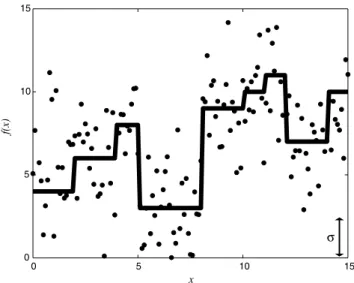
for each data set given by σ2(Figure1), can we identify partitions of
a (depth, other direction, or time) series with an underlying constant (i.e., mean) signal and so then identify the locations of the change points where the mean signal changes? We are not in a position to know in advance how many change points are appropriate, so we will estimate this from the data in the form of a transdimensional inference problem (Sambridge et al., 2006).
We may have some idea regarding the (possibly idealized) mea-surement errors for the downhole instruments, but we prefer not to make any assumptions regarding what parts of the varying data
series are signal and which are noise (Scales and Snieder, 1998). In this analysis, we initially consider all nonsignal variation in the data to be inferred as “noise,” noting that this may contain real signal, but not always the signal we are interested in. We will examine the in-terplay between different components of this variation. The total variation in the data may be expressed as
σ2T ¼ σ2 GPþ σ 2 GNþ σ 2 AN (1)
and is given by the sum of the variation due to the geologic process (GP), e.g., a dominant lithology change in which we are interested, the geologic noise (GN) due to natural variations of the observable (within a single dominant lithology) and the variation associated with errors in measurement procedures, analytic noise (AN) ( Gal-lagher et al., 2011). If we use transdimensional analysis primarily to determine a model (dominant lithology/depth structure), we would like our model to represent variations due to the GP without fitting variations internal to the dominant lithology at that depth (i.e., GN), or noise due to measurement error (i.e., AN): i.e., we do not wish to overfit the data. In this study, we are most interested in what the data themselves can tell us about the relative importance of noise due to GP, GN, and AN.
We use a Bayesian approach such that the unknowns are expressed in terms of probability density functions (Tarantola and Valette, 1982) with a simple statement of Bayes’ rule being
pðmjdÞ ∝ pðdjmÞpðmÞ; (2)
where pðmjdÞ is the posterior probability density function (PDF) of the unknown model parameter vector m, containing the unknowns, given the data vector d. The likelihood function pðdjmÞ is the prob-ability of the data being observed given the model and the prior probability density function, pðmÞ is a probability distribution
0 5 10 15 0 5 10 15 x f(x) σ
Figure 1. An example of the change-point problem for a single set of noisy data (dots), with a common noise level variance (redrawn fromGallagher et al., 2011). The noise has a normal distribution and the standard deviation (1 sigma, σ) is shown as the error bar in the bottom right. The underlying function from which the data were generated is shown by the solid line. The inference problem, using the observed data with an unknown noise level, is to estimate the distribution for the number and locations of the change points, and the variance of the noise distribution, from the noisy data.
reflecting what we think is reasonable to assume about the model parameters, in the absence of data. An accessible introductory reference for Bayesian data analysis is Sivia (1996), with more extensive reviews being provided byBernardo and Smith (1994)
andGelman et al. (2004). The approach is placed in the context of a broad survey of probability theory byJaynes (2003).
Our model vector m is such that
m¼ ðn; c; A; σÞ; (3)
where n is unknown number of change points and c is a vector of change points with ci, i¼ 1, n. There are n − 1 partitions separated
by these change points, with the mean of the data in the partition taking values given in the vector, A. The elements of A are Ailwith
i¼ 1, n − 1, and l ¼ 1, Nd, where n is the number of partitions and
Ndis the number of data sets (borehole logs in this case). Finally, for each data set, we assume the noise is random, comes from a normal distribution with a mean of zero and a variance of σ2, and the errors
are not correlated. As explained byMalinverno and Parker (2006), these assumptions lead to an error distribution with the most uncer-tainty. This variance of the noise distribution is a parameter to be inferred for each data set and again we follow the approach de-scribed inGallagher et al. (2011). Similar approaches to estimate the noise (uncorrelated and correlated) have been presented in sev-eral previous studies (Malinverno and Briggs, 2004; Malinverno and Parker, 2006;Bodin et al., 2012a).
Modeling of borehole geophysical data
Most borehole geophysical data interpretation is carried out by large petroleum companies using “in-house” software which is not in the public domain. Exceptions to this general pattern include, e.g., Petrolog (2008), Interactive Petrophysics (2010), and Log-Trans (Fullagar et al., 1999). With the increase in the use of bore-hole data for such applications as geothermal energy prospecting by junior (SME) companies, there is a growing need for the reinterpre-tation of public domain borehole geophysics data. Overviews of the common configurations of sondes, downhole geophysical data ac-quisition tools, are available (Dewan, 1983;Labo, 1987). Although these are not recent texts, they are relevant given that the public domain data which may warrant reinterpretation could have been acquired some time ago. In this case, the imperative for a robust and meaningful geophysical interpretation may be even greater if some of the matching drill core samples are now in poor condition or are otherwise unavailable.
The interpretation of observed borehole geophysics logs and in terms of lithology in commercial software, e.g., LogTrans (Fullagar et al., 1999) may be made through initial statistical characterization of a representative control data set. Discrimination of logs from si-milar formations are then made based on the nearest control class in multiparameter space. Within the Interactive Petrophysics software, there is a Monte Carlo simulation function which allows for some parameter sensitivity testing, however the user must provide error ranges. Our work here aims to add to such a practical analysis approaches. We use the data themselves to infer change points in the data series, and investigate the correlation between such change points and lithology boundaries/internal structure within lithologies. The errors are inferred from the data themselves and are not assumed before the uncertainty analysis. This may enable
additional insights to be made in data-rich environments, whereas for regions with sparse data and no control data sets, it may enable interpretations to be made which would not have been possible before. The analysis that we present in this study highlights the sensitivity of borehole geophysical logs to variations in lithology and the uncertainty inherent in using geophysical data to make predictions of lithology based on similar data.
Data and regional geologic setting
The borehole geophysical log data that we use were recorded in a well (Boyne River 2C) located in the Nagoorin Graben, in the north of the New England Orogen of East Australia (Glen, 2005;Howe, 2009;Slater, 2009). The region is prospective for hydrocarbon re-serves, with carbonaceous shales being discovered in a creek bank in 1885 and also for enhanced geothermal system style geothermal energy production. The petroleum lease is held by Arrow Energy Ltd., and the geothermal lease by Granite Power Ltd. The Nagoorin Graben is filled with a Tertiary sedimentary sequence, the Nagoorin Beds, which is almost entirely overlain by Quaternary alluvium (Henstridge and Hutton, 1987). The Nagoorin Beds comprise sand-stone with conglomerate and lignitic oil shale overlain by thick carbonaceous oil shale with intervals of mudstone, siltstone, and fine-grain sandstone. The depositional environment is interpreted to be lacustrine with some fluvial influence. The beds dip at 15° to the west and also include some later intrusive dolerite (Henstridge and Hutton, 1987;Murray and Blake, 2005;Cawood et al., 2011). Although the borehole geophysical logs and lithology logs were made for the purpose of hydrocarbon exploration, the subsequent identification of the Nagoorin Graben as a geothermal prospect has led to a reanalysis of the data on different terms. The oil shales and coal beds were of primary interest initially, with the rock ther-mal properties of the sedimentary sequence lithogies, and any inter-nal variation of these properties, now being of considerable interest. We use this combined borehole geophysical log and lithological log data set as an illustrative case: the lithology structure inferred from the change-point model can be compared and contrasted to the ac-tual lithology log, allowing us to assess the importance of different sources of variation in the data (as implied by equation1).
METHODS
We aim to generate an ensemble of values which approximate the posterior distribution of change points, expected borehole log values, and variance (although we present the square root of the variance). Because we do not know the number of change points in advance, our problem is transdimensional: that is, the number of model parameters is, in itself, an unknown which we estimate as part of the analysis. To solve this problem, we use a reversible jump MCMC sampling approach (Green, 1995,2003). There are recent applications of this technique and related approaches in earth sciences (Malinverno, 2002;Malinverno and Leaney, 2005;Jasra et al., 2006;Bodin and Sambridge, 2009;Charvin et al., 2009; Hop-croft et al., 2009; Agostinetti and Malinverno, 2010; Gallagher, 2012). In the description following, we briefly summarize the algo-rithm described byGallagher et al. (2011), which includes mathe-matical details in the supplementary material.
The MCMC sampling is an iterative process and proceeds by considering two sets of model parameters, the current and proposed models, mcand mp. The initial current model is chosen randomly
from the prior, and, at each iteration, the current model is perturbed to produce the proposed model. This step can be written as
mp¼ mcþ uσm; (4)
where σmis a scale factor vector for the model perturbation and u is
a random number vector drawn from an appropriate distribution (typically a normal distribution with a mean of zero and a variance of one). The scale factor needs to be chosen so that the sampler moves around the model parameter space in an efficient way. This proposed model is then accepted or rejected according to an accep-tance criterion, which includes a random component, such that ac-ceptance is more likely for a better data fit and rejection is more likely for a poorer data fit.
Acceptance is determined using the Metropolis-Hastings criter-ion defined as αðmp; mcÞ ¼ Min ! 1;pðmpÞpðdjmpÞqðmcjmpÞ pðmcÞpðdjmcÞqðmpjmcÞ " ; (5)
in which the first term in the ratio is the prior for each of the two models, the second term is the likelihood ratio, and the third term is the proposal function ratio. The likelihood function provides a mea-sure of the probability of the N observed data sets (d1; d2; : : : dN)
given the predictions from a given model m and is specified as
pðd1; d2: : : dNdjmÞ ¼ Y Nd l¼1 Y n i¼1 Y kil j¼1 1 ð2πσ2 lÞ 1 2 e− 1 2 # di;j;l−fi:lðxÞ σ l $2 ; (6)
where fi:lðxÞ is the predicted function value (the mean for out
pur-poses) for the data di:l, from the lth data set between the ith and the
i-lth change points with kil.
Intuitively, it may be expected that this process will lead to sam-pling progressively better data-fitting models which will tend to be more and more complex. However, the Bayesian approach avoids this, as complex models are penalized through the prior. This is a property known as “natural parsimony” (Jefferys and Berger, 1992;
Mackay, 1992;Malinverno, 2002;Jaynes, 2003).
After a number of iterations, known as the “burn-in,” the samples should then become representative of the posterior distribution (i.e., are drawn from the target posterior distribution). Accepted models from further postburn-in iterations are then used to infer the char-acteristics and uncertainties of the model ensemble. A representa-tive single model is given by the expected (or mean) model, rather than a best data-fitting model, with model parameter values at each depth x being given by a weighted mean of the posterior probability for each model parameter. When using multiple data sets, we as-sume that they all have common change-point locations, whereas the mean values between change points and the noise variance can differ for each data set. We use a uniform prior, with a limit on the number of change points between 1 and the number of data (401). The initial number of change points is taken to be 10% of the range and there is no minimum distance between change points, except that we do not allow more than one change point between any two data points, as they would not be constrained. The data are all zero-meaned and scaled to have unit variance (for each data set),
hence, a range of 0 to 1. All results are rescaled back to the appro-priate dimensions (units) for each data set for interpretation.
RESULTS
The results of the change-point modeling are shown (Figures2
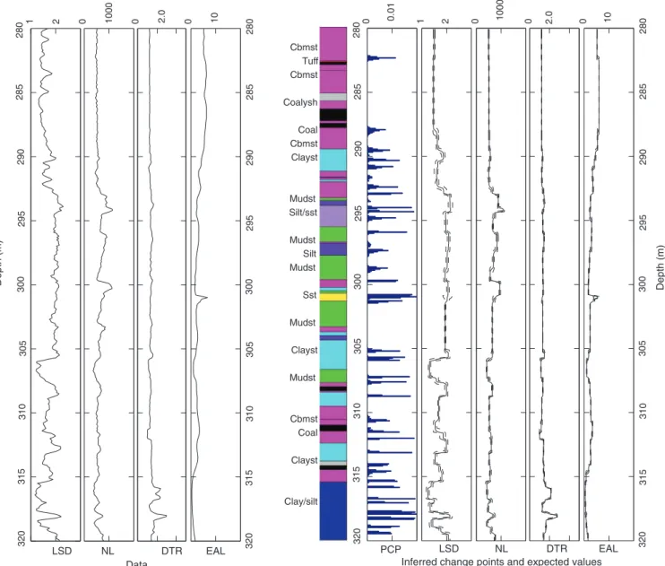
and3) together with the lithology log (center), the input data (left panels) and the expected models of the observed geophysical prop-erties and their upper and lower values (right panels). Figure 2
shows the results from the section of the borehole between 200 and 240 m, which includes intrusive igneous layers, and is charac-terized by high-contrast lithology boundaries and Figure3shows a group of lithologies from 280 to 320 m which are characterized by low-contrast lithology boundaries. The input sonic interval time log has been preprocessed to show delay time reciprocal (DTR) values which vary in the same sense as the long-spaced density (LSD) and other logs. Summary remarks on the characteristics of the interface between lithology pairs and on the internal variability of the litho-logical units (based on Figures2and3) are provided (Tables1and
2). In comparing the location and probability of the inferred change points with the recorded lithology, we can determine the informa-tion inherent in the geophysical response and anticipate strengths and shortcomings of using this information (i.e., these borehole logs) to determine lithology in other boreholes where logged core may not be available. In some cases, a peak in change-point prob-ability occurs at a lithology contact, in other cases there is a poor correspondence. Thus, we show the potential of using change-point modeling to highlight which boundaries can be identified, and which cannot, by the information contained within the bore-hole logs.
The change-point analysis highlights two properties of the lithol-ogy interfaces, as recorded in the response of the geophysical para-meters: the sharp/intermediate/broad location (i.e., resolution of the depth) of the change point and the strength of the contrast (i.e., the relative probability of a change point at a given depth). The coal layers are characterized by sharp, strong contrasts with silt and car-bonate mudstone (Table 1). Some interfaces between other sedi-mentary lithology pairs are generally broadly defined with weak contrasts, or seemingly absent in the geophysical response. Other interfaces between sedimentary lithology pairs (e.g., those with one unit being sandstone or silt) are sharply defined, and moderate or strong in contrast. Interfaces involving igneous lithologies are well-defined, with a weak contrast in geophysical response in the case of the tuff and a strong contrast in the case of the dolerite. The coal beds, coaly shale, and carbonate mudstone mostly show few internal change points (Table2), indicating low internal varia-bility at the resolution of the logging tools. There are, however, some exceptional cases such as the coal bed at 204 m which is strongly layered. Claystone, mudstone, sandstone, and silt units all show tightly defined internal change points indicating bedding which produces a strong response in the geophysical observables with no obvious change in lithology. Again, there are some excep-tions to this generalization, such as the mudstone unit between 301 and 303 m deep which shows little internal variability. The “stepped” appearance of the expected resistivity (EAL) model at the dolerite interfaces (200–205, 227–234 m on Figure 2), and the numerous implied change points, is considered an artifact of the model parameterization which we return to in the discussion section.
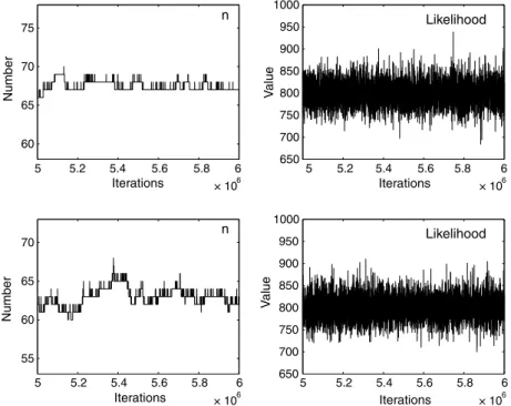
The transdimensional features of the MCMC sampling may be seen in the probability of the number of change points, n, which varies between 66 and 70 for the high contrast lithology sections and between 60 and 66 of the lower contrast section (Figure4). The variation in the number of change points, n, with iteration num-ber during the sampling, is represented (Figure 5) by the values from between five and six million iterations, well past the burn-in period of samplburn-ing, and representburn-ing part of the MCMC samplburn-ing of the posterior probability of the model parameter shown. Figure5
also shows the likelihood values along the same section of the chain. The lack of trends and the “fuzzy,” rather than “blocky,” char-acter to the likelihood value plots is an indication that the sampling
of the chain is stationary. In addition, we monitor the acceptance rates for each parameter type. For each of the four logs, we have the location of the change points, the change-point mean, and the noise variance, as well as the number of change points. Generally, an acceptance rate of 0.15–0.5 indicates that the stationary distribution has been sampled efficiently (e.g., Roberts and Rosenthal, 2001).
The distributions of the variance of the noise for each geophysical observable are shown as histograms (Figure 6). The noise is as-sumed, as for many physical problems, to be represented by a zero-mean normal distribution and the parameter that we estimate is the variance of that normal distribution. We infer a distribution on
200 205 210 215 220 225 230 235 240 0 20 0 4.0 0 1000 200 205 210 215 220 225 230 235 240 1 2 200 205 210 215 220 225 230 235 240 0 20 0 0 1000 1 2 200 205 210 215 220 225 230 235 240 0 0.01 0.02 Data Depth (m) PCP
Inferred change points and expected values EAL DRT NL LDS L A E R T D L N D S L Depth (m) 4.0 Dolerite Coal Silt Coal Coalysh Coal Cbmst Clayst Coalysh (coreloss) Sst Silt Coalysh Cbmst Dolerite Cbmst (coreloss) Cbmst Coal Cbmst Clayst x x x
Figure 2. Borehole geophysical log data from a well near Ubobo, Queensland, Australia (Boyne River 2C) and results of the change-point analysis. The depth interval, 200–240 m, is characterized by strong lithological contrasts. The observed data are the logs on the left hand side: LSD (g∕cm3), Neutron Log (NL; counts), DTR (equivalent to seismic velocity [km∕s]), and electrical array log (ohm-m). PCP¼
ðposteriorÞ probability of change point represented by the bars on the right of the lithology log. The panels on the right show the inferred structure for the expected model (the mean of the predicted values between each change-point pair) and the dashed lines represent the 95% credible intervals about the expected values. Lithology abbreviations are given in Table1. Lithologies are shown by color, with thicker units and some mixed lithology units annotated beside the log. Coal¼ black, coalyshale ¼ gray, carbonate mudstone ¼ magenta, claystone ¼ cyan, sandstone¼ yellow, silt ¼ purple, dolerite ¼ dark orange, tuff ¼ red, coreloss ¼ pale yellow (marked x).
that parameter, with a form dependent on the information in the data. The upper plots show the total noise variance distributions for the high-contrast section and the lower plots show total noise values for the low-contrast section. In plotting the total noise var-iance, we are combining the variances over different lithologies (i.e., we do not distinguish in these summary plots between strata with different GN). The plots effectively show the variance due to the high-frequency internal variability in the dominant lithology of each section and hence provide a maximum value for the AN. The x-axis values differ for each of the two sections, but the x-axis ranges (maximum value to minimum value) for each parameter are the same, to facilitate comparison between the two sets of plots. The mean value of noise variance, and also the range in this para-meter, inferred for the neutron (porosity), seismic velocity, and electrical resistivity logs (NL, DTR, and EAL) is greater for the
high-contrast section. The range in noise parameter for the LSD is slightly wider for the low-contrast section, and the mean some-what higher, due to the high density variability within some lithol-ogies. We explore further details of the inferred noise parameter values in the discussion that follows.
DISCUSSION
We first consider the likely contributions to the varying variation between the lithological structure, uncertainty and the noise inferred at different depths and for the different lithologies. Following this appraisal, we discuss practical aspects of the data collection and some possible refinements for using transdimensional inference to investigate uncertainty in applied geophysics.
Considering equation1, which separates the sources of variabil-ity in the input data into those due to GP, GN, and AN, we now
Data
Depth (m)
Inferred change points and expected values
NL EAL PCP NL EAL 0 10 0 0 1000 1 2 280 285 290 295 300 305 310 315 320 0 0.01 0 10 0 2.0 0 1000 280 285 290 295 300 305 310 315 320 1 2 280 285 290 295 300 305 310 315 320 280 285 290 295 300 305 310 315 320 Depth (m) Cbmst Tuff Cbmst Coalysh Coal Cbmst Clayst Mudst Silt/sst Mudst Silt Mudst Sst Mudst Clayst Mudst Cbmst Coal Clayst Clay/silt Depth (m) 2.0 LSD DTR LSD DTR
Figure 3. Borehole geophysical log data from a well near Ubobo, Queensland, Australia (Boyne River 2C) and results of the change-point analysis for the depth interval, 280–320 m. This part of the sedimentary sequence is characterized by lower contrasts in geophysical properties than the section shown in the previous figure. See the caption to Figure2for geophysical borehole log mnemonics, other abbreviations, and details.
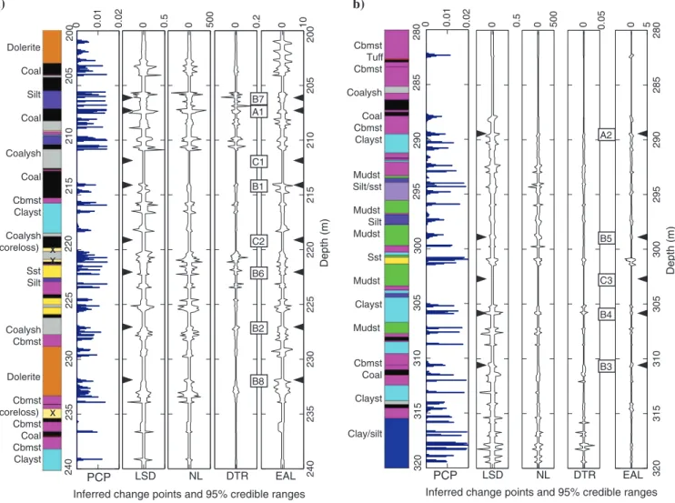
examine the noise variability with depth in our two sections of bore-hole and associated geophysical logs (Figure7). In this figure, we have plotted the 95% credible interval on the inferred mean values between partitions. Credible intervals are the Bayesian equivalent of the more well-known confidence intervals, although their interpre-tation is somewhat different, being the specified probability range of the posterior distribution for a given model parameter (seeBernardo and Smith [1994]for a discussion). The mean values can change during the sampling as the change-point structure (and so the data contained between two change points) changes. The credible inter-val range therefore reflects the resolution of the mean inter-values as a function of depth. Note that these credible intervals have been plotted after removing the expected model (i.e., zero meaned). The change points which correspond to GP variations, or lithology boundaries identified in the visual log often show relatively large 95% credible intervals where the probability distribution for a
change point is relatively diffuse, or broad. This could reflect a lack of depth resolution on a single change point, or that we are dealing with several closely spaced change points. Two examples are indi-cated for a strong and weaker contrast (e.g., A1 and A2: Table1and Figure7). In borehole geophysical analysis, such changes are the desired structural variations in the model. We wish to be able to distinguish between variations due to GP (our signal, the dominant lithological structure) and those due to GN and AN (noise or signal we are not interested in, e.g., geophysical variation within a single lithology or AN/measurement error).
Further consideration of change-point structure, and variation in the credible interval ranges, provides some insight into the likely GN variations (B1–B8: Table2and Figure7). Claystone, mudstone, sandstone, and silt lithologies clearly show that they are likely to give rise to a GN response in the geophysical logs. The magnitude of this noise is as large, and may be larger (e.g., B7) than the sought-after response reflecting the dominant GP. Table2shows represen-tative values for the GN response for all the main lithologies in this study. This is information which could be extremely valuable in preparing data for, and interpreting the results of lithology classi-fications from other software. The inferred values of the square root of the variance, σ, where there are no change points or lithology changes provide a maximum limit on the practical AN response of the geophysical logs. Two examples are given, C1 and C3, for the high- and low-contrast lithology sections (Figure7). At these points, there are neither changes in lithology identified in the visual log (i.e., no GP response) nor change points within a lithology (i.e., no strong GN response). These values are good indications of the Table 1. Summary of the characteristics of lithology
interfaces highlighted by the change-point (CP) analysis. cbmst ! carbonate mudstone, clayst ! claystone,
mudst ! mudstone, sst ! sandstone, coalysh ! coalyshale.
Lithology 1 Lithology 2
Interface characteristic Sharp/intermediate/
broad CP location Strong/moderate/weak contrast
Coal Silt Sharp Strong
Coal cbmst Sharp Moderate
coalysh Coal Absent —
coalysh cbmst Broad or absent Weak
cbmst clayst Broad or absent Weak or moderate (e.g., A2, 289 m)
clayst coalysh Intermediate Moderate
clayst mudst Absent —
mudst cbmst Sharp Moderate
sst Silt Sharp Moderate
sst mudst Sharp Moderate
Silt Coal Sharp Strong (e.g., A1,
207 m)
Silt mudst Sharp Moderate
Tuff Coal/cbmst Sharp Weak
Dolerite Coal Intermediate Strong
Dolerite cbmst Intermediate Strong
Table 2. Summary of internal variability of significant lithologies as highlighted by the change-point analysis. Lithology names are given in the caption to Table1.
Lithology Internal variability Example
Coal Most beds show low internal variability.
A few beds layered B1
coalysh Low internal variability B2
cbmst Low internal variability B3
clayst Thick, well-defined beds B4
mudst Thick, well-defined beds. Some
show low internal variability B5
sst Strongly bedded B6
Silt Strongly bedded B7
Dolerite Mostly low internal variability.
Some porosity variation B8
60 65 70 75 0 0.1 0.2 0.3 0.4 0.5 0.6 55 60 65 70 0 0.1 0.2 0.3 0.4 0.5 0.6 Probability
n, number of change points
Probability
n, number of change points
200-240 m 280-320 m Figure 4. Posterior distributions of the parameter
n, number of change points (see equation3), for the high-contrast section (200–240 m, left) and the low contrast section (280–320 m, right) of the borehole log.
effective AN response, the practical uncertainty in the measuring system, taking all factors into consideration. Example C2 shows a counterexample, where no change points are identified, but there are lithology changes in the visual log (although not extreme, the lithologies being coal or coaly shale). The values for the AN re-sponses in this case, across the four geophysical logs, are clearly greater than the example at C1. If we assume that the AN response
of the measuring systems is constant, then we can interpret these greater values of σ (C2 in comparison to C1) to include a compo-nent of GP and GN response. In this case the geologic response, be it “process” or “noise” is below the level at which our method infers a change point, reflecting the information contained in the data about such changes.
In this study, our goal is to investigate the uncertainty in the logs with a view to subsequently using similar infor-mation to infer lithology in similar boreholes which may have been drilled without preserving the core. Our analysis shows clearly which litho-logical contrasts correspond with a statistically detectable response in the geophysical logs and those which are much less likely to be in-ferred from the geophysical data. It also allows a maximum value for the AN response to be de-termined. We also provide a quantitative apprai-sal of the GN response for each lithology. We note that the GN response (e.g., B4 and B7) may be very strong, and often associated with a change point that is tightly defined in depth (showing as a narrow range in the probability of change-point depth plots). Thus, a representa-tive section of a borehole may be used to explore the uncertainties in the available data and an overall appraisal of the sensitivity of the geophy-sical response to the change in lithologies, i.e., the desired inference goal in the routine analysis of similar data from many other boreholes.
The sondes (downhole tools) used to acquire borehole geophysical log data are often 1–2 m or more in length, recording measurements, as in the data we use in this demonstration, at 0.1-m intervals. This has the advantage of redu-cing short wavelength noise, produredu-cing a re-sponse that is a more faithful representation of
× 106 60 65 70 75 × 106 650 700 750 800 850 900 950 1000 5 5.2 5.4 5.6 5.8 6 × 10⁶ 55 60 65 70 5 5.2 5.4 5.6 5.8 6 × 10⁶ 650 700 750 800 850 900 950 1000 Likelihood Likelihood n n Iterations Iterations Iterations Iterations 5 5.2 5.4 5.6 5.8 6 5 5.2 5.4 5.6 5.8 6 Number N um b er V a lue V alue
Figure 5. An example of the transdimensional sampling for the number of change points (n) and the log likelihood values (better data fitting models have higher log likelihood values) taken from a section of the Markov chain between 5 and 6 million iterations for the high contrast section (200–240 m, upper plots) and the low-contrast section (280– 320 m, lower plots) of the borehole log.
Probability Probability Probability Probability Probability Probability Probability Probability 0.1 0.2 0.3 0.1 0.2 0.3 0.4 0.5 0.1 0.2 0.3 0.08 0.09 0.1 0.11 0.1 0.2 0.3 40 50 60 70 0.1 0.2 0.3 0.06 0.07 0.08 0.09 0.1 0.2 0.3 40 50 60 70 0.1 0.2 0.3 0..08 0.1 0.12 0.1 0.2 0.3 0. 1.0 1. 1 1. 1. 0.1 0.2 0.3 LSD LSD NL NL DTR DTR EAL EAL σ (g/cm3) σ (g/cm3) σ (counts) σ (counts) σ (g/cm3) σ (g/cm3) σ (ohm-m) σ (ohm-m) 9 2 3 0.14 0.08 0.06 0.02 0.04
Figure 6. Posterior distributions of the noise parameter (shown here as the standard deviation of the noise distribution) for each borehole geophysical log observable in the high-contrast section (200–240 m, upper plots) and the low-contrast section (280–320 m, lower plots) of the borehole log. See the caption to Figure2for geophysical borehole log mnemonics.
the bulk rock property (e.g., density). The disadvantage can be that recorded values are smeared or averaged as the sonde passes over lithological contacts. The inferred σ value due to a change in lithol-ogy is influenced by the sonde length. In this work, we are not at-tempting to replicate the physics of the data acquisition process, as in a deterministic modeling process, we are using the underlying variations in the observed data, from wherever they might arise, to understand how the observed data relate to what we might want to infer. Hence, the exact mechanism of the change in σ is not im-portant, so long as similar sondes are used collecting the data sets for the transdimensional change-point uncertainty analysis and the subsequent routine processing.
In the method presented here, we have restricted the modeled values of the geophysical logs between change points (contained in the vector A, equation3) to be constant values (i.e., a zeroth order polynomial). This constraint may be relaxed through the use of a higher-order regression function (e.g., a polynomial) between change points (Gallagher et al., 2011). For example, a first-order
polynomial, rather than a constant value, would remove the multiple step structures (implying multiple, closely spaced change points) occasionally evident where there are steep gradients over a rela-tively long proportion of the data series (e.g., the EAL at 202 and 228 m). Indeed, in a more general case, the order of the poly-nomial between pairs of change points may itself be treated as a parameter to be estimated. Our emphasis in this work is the identi-fication and analysis of the way in which the noise variance changes with the visual dominant lithology log, hence, provided such multi-ple steps are not misidentified as internal change points, the simmulti-pler analysis procedure using constant values between change points re-mains appropriate. It is worth noting that the expected model is ef-fectively a smoothed version of many individual models which are all just a series of constants between change points. However, the expected model can be more complex in that it can have gradients (due to smoothing) and so potentially capture subtle transitions be-tween two lithologies better than an individual model taken from the sampled ensemble (e.g., the best data-fitting model).
PCP
Inferred change points and 95% credible ranges LSD NL DTR EAL 280 285 290 295 300 305 310 315 320 0 0.01 280 285 290 295 300 305 310 315 320 0 5 0 0 500 0 0.5 200 205 210 215 220 225 230 235 240 0 0.01 0.02 0.02 PCP
Inferred change points and 95% credible ranges LSD NL DTR EAL 200 205 210 215 220 225 230 235 240 0 10 0 0.2 0 500 0 0.5 B7 C1 C2 A1 A2 B5 B1 B2 B8 B6 B4 B3 C3 Dolerite Coal Silt Coal Coalysh Coal Cbmst Clayst Coalysh (coreloss) Sst Silt Coalysh Cbmst Dolerite Cbmst (coreloss) Cbmst Coal Cbmst Clayst x x x Cbmst Tuff Cbmst Coalysh Coal Cbmst Clayst Mudst Silt/sst Mudst Silt Mudst Sst Mudst Clayst Mudst Cbmst Coal Clayst Clay/silt Depth (m) Depth (m) 0.05 a) b)
Figure 7. Inferred change points plotted with the 95% credible interval ranges for (a) the high-contrast section (200–240 m) and (b) the low-contrast section (280–320 m) of the borehole log. Indicated by the labels between the logs DTR and EAL, A1 and A2 (also noted in Table1) are examples of variation due to GP, i.e., changes in the dominant lithology. B1–B7 (also noted in Table2) are examples of GN, i.e., variation due to internal variation in each lithology. C1–C3 are examples of log sections with no change points that provide an insight into the level of AN i.e., measurement error. See the caption to Figure2for geophysical borehole log mnemonics, other abbreviations and details.
CONCLUSION
Transdimensional change-point analysis may be used to make an appraisal of the inferred lithology, depth structure, and noise contributions from a representative section of stratigraphy and the associated geophysical logs. The appraisal provides an insight into the noise in the data due to GP (variation between dominant lithologies), GN (variation within a lithology) and analytical (mea-surement) noise. Thus, the varying sources of uncertainty in the data, and hence the ability of the geophysical data to constrain lithology in subsequent analysis, can be investigated directly as part of the inference process. This approach could be employed in the routine processing of borehole geophysical log data to gain a pre-liminary understanding, from one representative section, of the abil-ity of the data to constrain the anticipated lithology contrasts in other wells. The approach would generalize readily to any geo-physical investigation where one or more noisy data series is used to infer a model with contrasts in structure along a section, or with depth.
ACKNOWLEDGMENTS
Borehole geophysical log data and reports were sourced from the Queensland Department of Mines and Energy QDEX system, Aus-tralia. Background geologic and borehole geophysical log informa-tion were partly researched by Michelle Slater and Stephanie Howe as part of their Honours project (and/or following work) at UTAS. Granite Power Ltd. is thanked for their support of student projects at UTAS including those of M. Slater and S. Howe. We thank three anonymous reviewers for their constructive comments which im-proved the content and clarity of the manuscript.
REFERENCES
Agostinetti, N. P., and A. Malinverno, 2010, Receiver function inversion by trans-dimensional Monte Carlo sampling: Geophysical Journal Interna-tional, 181, 858–872.
Bernardo, J., and A. F. M. Smith, 1994, Bayesian theory: John Wiley and Sons Ltd.
Bodin, T., and M. Sambridge, 2009, Seismic tomography with the reversible jump algorithm: Geophysical Journal International, 178, 1411–1436, doi:
10.1111/j.1365-246X.2009.04226.x.
Bodin, T., M. Sambridge, N. Rawlinson, and P. Arroucau, 2012a, Transdi-mensional tomography with unknown data noise: Geophysical Journal International, 189, 1536–1556, doi:10.1111/j.1365-246X.2012.05414.x. Bodin, T., M. Sambridge, H. Tkalcic, P. Arroucau, K. Gallagher, and N. Rawlinson, 2012b, Transdimensional inversion of receiver functions and surface wave dispersion: Journal of Geophysical Research Solid Earth : JGR, 117, B02301, doi:10.1029/2011JB008560.
Cawood, P. A., S. A. Pisarevsky, and E. C. Leitch, 2011, Unraveling the New England orocline, east Gondwana accretionary margin: Tectonics, 30, TC5002, doi:10.1029/2011TC002864.
Charvin, K., K. Gallagher, G. L. Hampson, and R. Labourdette, 2009, A Bayesian approach to inverse modelling of stratigraphy, part 1: Method: Basin Research, 21, 5–25, doi:10.1111/j.1365-2117.2008.00369.x. Denison, D. G. T., C. C. Holmes, B. K. Mallick, and A. F. M. Smith, 2002,
Baysian methods for nonlinear classification and regression: John Wiley and Sons Ltd.
Dewan, J. T., 1983, Modern open-hole log interpretation: Pennwell Books. Dosso, S. E., and J. Dettmer, 2011, Bayesian matched-field geoacoustic in-version: Inverse Problems, 27, 055009, doi:10.1088/0266-5611/27/5/ 055009.
Fullagar, P. K., B. Zhou, and G. N. Fallon, 1999, Automated interpreta-tion of geophysical borehole logs for orebody delineainterpreta-tion and grade estimation: Mineral Resources Engineering, 8, 269–284, doi:10.1142/ S095060989900027X.
Gallagher, K., 2012, Transdimensional inverse thermal history modeling for quantitative thermochronology: Journal of Geophysical Research Solid Earth: JGR, 117, B02408, doi:10.1029/2011JB008825.
Gallagher, K., T. Bodin, M. Sambridge, D. Weiss, M. Kylander, and D. Large, 2011, Inference of abrupt changes in noisy geochemical records using transdimensional changepoint models: Earth and Planetary Science Letters, 311, 182–194, doi:10.1016/j.epsl.2011.09.015.
Gelman, A., J. Carlin, H. Stern, and D. Rubin, 2004, Bayesian data analysis, 2nd Edition: Chapman and Hall.
Glen, R. A., 2005, The Tasmanides of eastern Australia, in A. P. M. Vaugh-an, P. T. Leat, and R. J. Pankhurst, eds., Terrance processes at the margins of Gondwana: Geological Society of London Special Publications, 246, 23–96.
Green, P. J., 1995, Reversible jump Markov chain Monte Carlo computation and Bayesian model determination: Biometrika, 82, 711–732, doi: 10 .1093/biomet/82.4.711.
Green, P. J., 2003, Transdimensional MCMC, in P. J. Green, N. Hjort, and S. Richardson, eds., Highly structured stochastic systems: Oxford Statistical Science Series, 179–196.
Guo, R. W., S. E. Dosso, J. X. Liu, J. Dettmer, and X. Z. Tong, 2011, Non-linearity in Bayesian 1-D magnetotelluric inversion: Geophysical Journal International, 185, 663–675, doi:10.1111/j.1365-246X.2011.04996.x. Henstridge, D. A., and A. C. Hutton, 1987, Geology and organic
petrogra-phy of the Nagoorin oil-shale deposit: Fuel, 66, 301–304, doi:10.1016/ 0016-2361(87)90082-2.
Hopcroft, P. O., K. Gallagher, and C. C. Pain, 2009, A Bayesian partition modelling approach to resolve spatial variability in climate records from borehole temperature inversion: Geophysical Journal International, 178, 651–666, doi:10.1111/j.1365-246X.2009.04192.x.
Howe, S., 2009, Deriving rock thermal properties from wireline well logs and comparisons to values measured on drill core: Honours thesis, University of Tasmania.
Interactive Petrophysics, 2010, Senergy software,http://www.senergyworld .com/software/interactive-petrophysics, accessed 15 January 2013. Jasra, A., D. A. Stephens, K. Gallagher, and C. C. Holmes, 2006, Bayesian
mixture modelling in geochronology via Markov chain Monte Carlo: Mathematical Geology, 38, 269–300, doi:10.1007/s11004-005-9019-3. Jaynes, E. T., 2003, Probability theory, the logic of science: Cambridge
Uni-versity Press.
Jefferys, W. H., and J. O. Berger, 1992, Ockham’s razor and Bayesian ana-lysis: American Scientist, 80, 64–72.
Labo, J., 1987, A practical introduction to borehole geophysics: SEG. Li, Y. G., and D. W. Oldenburg, 1998, 3-D inversion of gravity data:
Geophysics, 63, 109–119, doi:10.1190/1.1444302.
Li, Y. G., and D. W. Oldenburg, 2000, 3-D inversion of induced polarization data: Geophysics, 65, 1931–1945, doi:10.1190/1.1444877.
Loke, M. H., and R. D. Barker, 1996, Practical techniques for 3D resistivity surveys and data inversion: Geophysical Prospecting, 44, 499–523, doi:
10.1111/j.1365-2478.1996.tb00162.x.
Loke, M. H., P. B. Wilkinson, and J. E. Chambers, 2010, Parallel computa-tion of optimized arrays for 2-D electrical imaging surveys: Geophysical Journal International, 183, 1302–1315, doi:10.1111/j.1365-246X.2010 .04796.x.
Mackay, D. J. C., 1992, Bayesian interpolation: Neural Computation, 4, 415–447, doi:10.1162/neco.1992.4.3.415.
Malinverno, A., 2002, Parsimonious Bayesian Markov chain Monte Carlo inversion in a nonlinear geophysical problem: Geophysical Journal Inter-national, 151, 675–688, doi:10.1046/j.1365-246X.2002.01847.x. Malinverno, A., and V. A. Briggs, 2004, Expanded uncertainty
quantifica-tion in inverse problems: Hierarchical Bayes and empirical Bayes: Geo-physics, 69, 1005–1016, doi:10.1190/1.1778243.
Malinverno, A., and W. S. Leaney, 2005, Monte-Carlo Bayesian look-ahead inversion of walkaway vertical seismic profiles: Geophysical Prospecting, 53, 689–703, doi:10.1111/j.1365-2478.2005.00496.x.
Malinverno, A., and R. Parker, 2006, Two ways to quantify uncertainty in geophysical inverse problems: Geophysics, 71, no. 3, W15–W27, doi:10 .1190/1.2194516.
Murray, C. G., and P. R. Blake, 2005, Geochemical discrimination of tec-tonic setting for Devonian basalts of the Yarrol Province of the New Eng-land Orogen, central coastal QueensEng-land: An empirical approach: Australian Journal of Earth Sciences, 52, 993–1034.
Petrolog, 2008, Advanced log analysis software, http://petrolog.net, ac-cessed 15 January 2013.
Roberts, G., and J. Rosenthal, 2001, Optimal scaling for various Metropolis-Hastings algorithms: Statistical Science, 16, 351–367, doi:10.1214/ss/ 1015346320.
Sambridge, M., 1999, Geophysical inversion with a neighbourhood algo-rithm — II. Appraising the ensemble: Geophysical Journal International, 138, 727–746, doi:10.1046/j.1365-246x.1999.00900.x.
Sambridge, M., K. Gallagher, A. Jackson, and P. Rickwood, 2006, Trans-dimensional inverse problems, model comparison and the evidence: Geophysical Journal International, 167, 528–542, doi: 10.1111/j.1365-246X.2006.03155.x.
Scales, J. A., and R. Snieder, 1998, What is noise?: Geophysics, 63, 1122– 1124, doi:10.1190/1.1444411.
Sen, M. K., and P. L. Stoffa, 1992, Rapid sampling of model space using genetic algorithms — examples from seismic waveform inversion: Geo-physical Journal International, 108, 281–292, doi:10.1111/j.1365-246X .1992.tb00857.x.
Sivia, D. S., 1996, Data analysis: A Bayesian tutorial: Clarendon Press. Slater, M. A., 2009, Appraisal of the enhanced geothermal system potential
of the Nagoorin Graben, Queensland: Honours thesis, University of Tasmania.
Stoffa, P. L., and M. K. Sen, 1991, Nonlinear multiparameter optimisation using genetic algorithms: Inversion of plane-wave seismograms: Geo-physics, 56, 1794–1810, doi:10.1190/1.1442992.
Tarantola, A., and B. Valette, 1982, Inverse problems = quest for informa-tion: Journal of Geophysics, 50, 159–170.
Wu, Z., N. E. Huang, S. R. Long, and C. K. Peng, 2007, On the trend, detrending and variability of nonlinear and nonstationary time series: Proceedings of the National Academy of Sciences of the United States of America, 104, 14889–14894.
Yamanaka, H., and H. Ishida, 1996, Application of genetic algorithms to an inversion of surface-wave dispersion data: Bulletin of the Seismological Society of America, 86, 436–444.
Zelt, C. A., and P. J. Barton, 1998, Three-dimensional seismic refraction tomography: A comparison of two methods applied to data from the Faeroe Basin: Journal of Geophysical Research Solid Earth: JGR, 103, 7187–7210, doi:10.1029/97JB03536.