HAL Id: halshs-00570491
https://halshs.archives-ouvertes.fr/halshs-00570491
Preprint submitted on 28 Feb 2011
HAL is a multi-disciplinary open access archive for the deposit and dissemination of sci-entific research documents, whether they are pub-lished or not. The documents may come from teaching and research institutions in France or abroad, or from public or private research centers.
L’archive ouverte pluridisciplinaire HAL, est destinée au dépôt et à la diffusion de documents scientifiques de niveau recherche, publiés ou non, émanant des établissements d’enseignement et de recherche français ou étrangers, des laboratoires publics ou privés.
What is the Role of Openness for China’s Environment?
An Analysis Based on Divisia Decomposition Method
From the Regional Angle
Jie He
To cite this version:
Jie He. What is the Role of Openness for China’s Environment? An Analysis Based on Divisia Decomposition Method From the Regional Angle. 2011. �halshs-00570491�
Fifth Chinese Economy Conference of CERDI (20-21 Oct, 2005)
WHAT IS THE ROLE OF OPENNESS FOR CHINA’S ENVIRONMENT? AN ANALYSIS BASED ON DIVISIA DECOMPOSITION METHOD FROM THE
REGIONAL ANGLE
Jie Heψ
Observing the weakness in the previous structural analyses on EKC formation, in this paper, author deepens the analysis into the detailed data of production and SO2 emission intensity of China’s 29 industrial sectors (occupying over 98% of the total industrial production) in each province during 1991-2001. With the aid of Divisia Index Decomposition method, the variation of the provincial-level industrial SO2 emission with regard to the original level of 1990 is decomposed into the contribution from its three determinants: the variations in its production scale, its composition transformation and its technique character changes. The following analysis aims to reveal regional differences in environmental impact of industrialization and to further interrogate the potential links between these region-specific environmental impacts of industrialization and development of commercial openness in each province.
Key Words: Openness, pollution, China, Decomposition, region.
1. Introduction
Most of the literatures aiming at explaining the formation of the Environmental Kuznets Curve in an economy generally agree with the Grossman (1995) decomposition and distinguish the determination role played by its scale, composition (structure) and technique characters. Although originally the composition effect is to describe the actual pollution performance of the economy’s industrial structure, constrained by data availability, most of existing literature on this topic employed the capitalistic ratio (or the capital abundance degree) calculated as the total capital employed in production divided by total labor (K/L). As generally (or traditionally) polluting heavy industries employ more capital in their production, the common sense suggests that we can use this capitalistic ratio as an approximation for environmental performance of the industrial structure of an economy and suppose higher capitalistic ratio means more intensive polluting industry concentrated in economy. However, the rise of the knowledge and high-tech industries during the last several decades obviously disrupts this assumption, since the production process of most of the capital-intensive new high-tech industries, as the information industry, are not polluting at all.
Observing the weakness in the measurement of composition effect, in this paper, author deepens the analysis into the detailed data of production and SO2 emission intensity of China’s 29 industrial sectors (occupying over 98% of the total industrial production) in each province during 1991-2001. With the aid of Divisia Index Decomposition method, the variation of the provincial-level industrial SO2 emission with regard to the original level of 1990 is decomposed into the contribution from its three determinants: the variations in its production scale, its composition transformation and its technique character changes. The following analysis aims to reveal regional differences in environmental impact of industrialization and to further interrogate the potential links between these region-specific environmental impacts of industrialization and development of commercial openness in each province.
The organization of the paper is as following, in section 2 we introduce the Grossman Decomposition and then we show in section 3 how the Grossman decomposition can be related to the Divisia index decomposition method and how we need to adapt the Divisia index decomposition method to China’s data. The decomposition results that distributed the variations of China’s industrial SO2 emission into the contribution from scale enlargement, structural transformation and technical progress during 1991-2001 are then discussed in section 4. Following in section 5, we employ the decomposed contribution of the three
structural determinants in emission variation to investigate the potential impact of international trade on industrial SO2 emission via these three determinants. Finally, we conclude in section 6.
2. Grossman Decomposition
Most theoretical explanations for EKC formation base their reasoning on the demand-side factor. These analyses generally condemand-sider the decoupling of economic growth and environmental deterioration as the result of the trade-off between utility from normal good consumption and disutility caused by pollution. However, demand-side causes are only the necessary conditions for the appearance of EKC turning point. Without satisfying certain supply-side conditions, such as technological capacities in pollution abatement or production process and the de-pollution trends in industrial structure transformation, a simple rise of public demand for a better-environment may only lead economic growth to a halt and cannot realize a win-win result. As this paper is interested in industrial SO2 emission situation in China, a developing country, whose most important objective is still to enrich its population at the moment, the analyses on the supply-side emission determination factors are actually more appropriate.
More or less, based on macroeconomic foundation, some theoretical analyses have already involved in their discussion the supply-sides pollution determinants and explored the structural explanation for the formation of EKC. The most widely accepted supply-side pollution determinants are those proposed by Grossman (1995), which regarded pollution as a by-product of production activities. According to him, the final total emission results can be calculated by equation (1).
∑
= = n 1 j t, j t, j t t Y I S E (1) Where Et means the emission in year t. j=1,2,…,n represents the different sectors in the economy, Yt is the total GDP in year t, it can also be presented by the sum of value added of the n sectors, so Yt=ΣYj,t. Ij,t is the emission intensity, the average quantity of pollution emitted for each unit of product in sector j, so Ij,t=Ej,t/Yj,;t. Sj,t=Yj,t/Yt, it represents the ratio of the value added of sector j in total GDP. According to this equation, total emission can be considered as product of the total value added of economy Yt and the average sectoral emission intensity weighted by the ratio of each sector’s GDP in total economy Σj(Ij,tSj,t).If we make total differentiation with respect to time and then divide the whole equation by total emission results, E, we reproduce the Grossman decomposition in equation (2).
∑
∑
+ + = j j j j j jS e I e Y E^ ^ ^ ^ (2)Where ej=Ej/E represents the ratio of emission from sector j in total economy and
} Y , S , I, E { X , X / ) dt / dX ( X t ^ ∈
= . This decomposition defines the famous three determinants of emission. Y denotes the scale effect, which is expected to be a pollution-increasing factor.^ “All else equal, an increase in output means an equiproportionate increase in pollution”. The composition effect is represented by S^j, the changes in Sj over time represent the influence on emission of a change in the composition of economic activities. All else equal, if the sectors with high emission intensities grow faster than sectors with low emission intensities, the composition changes will result in a upwards pressure on emission, so that total emission will grow at a faster rate than income. ^Ij represents the technique effect. The decrease in sector
emission intensities, as the results of the use of more efficient production and abatement technologies, can reduce emission increasing pressure given the same quantity of economic growth and fixed industrial composition mix.
Grossman decomposition is actually based on the decomposition principal of Divisia, in the following sector, we will explain in details about the decomposition steps.
3. Linkage between the Grossman decomposition to Divisia index decomposition method
3.1. The origin of Divisia index
The Divisia index is a continuous time index number formula due to François Divisia (1925). This index has already been widely used in theoretical discussions of data aggregation and the measurement of technical change. It is defined with respect to the time paths of set variables. For example, at given period t, the prices [P1(t), P2(t), P3(t),…, PN(t)] and commodities [X1(t), X2(t), X3(t),…, XN(t)]. Total expenditure on this group of commodities is given by:
Y(t)=P1(t)X1(t)+P2(t)X2(t)+P3(t)X3(t)+…+PN(t)XN(t). (3) Using dots over variables to indicate derivatives with respect to time, the total differentiation of (3) yields:
∑
∑
= • = • • + = N 1 i i i i i N 1 i i i i i ) t ( X ) t ( X ) t ( Y ) t ( X ) t ( P ) t ( P ) t ( P ) t ( Y ) t ( X ) t ( P ) t ( Y ) t ( Y . (4)The first summation of the right-hand side of (4) defines the Divisia index of prices and the second defines the Divisia quantity index. Both indexes are weighted averages of the growth rates of the individual Pi(t) and Xi(t), where the weights are the components’ shares in total expenditures: Pi(Yt)(Xt)i(t).The sum of equation (4) thus defines the rate of change of the aggregate price and quantity indexes. The levels of these indexes are obtainable by line integration over the trajectory followed by the individual prices and quantities over the time interval [0,T]. For the quantity index, the line integral has the following form:1
{
∫
[
∑
]
}
= • = N 1 i i i i i q ) t ( X ) t ( X ) t ( Y ) t ( X ) t ( P exp ) T , 0 ( I . (5)We note that the Divisia index is defined using time as a continuous variable. This is actually not appropriate for empirical analysis, where the data on both price and quantity typically refer to discrete points in time.
To resolve this problem, we need to approximate the continuous variables of equation (4) with their discrete time counterparts. The approach of Törnqvist (1936) suggests approximating the growth rate of prices and quantities by logarithmic differences and the continuous weights by two periods arithmetic averages. So the Törnqvist approximation to the growth rate of the Divisia quantity index can then be written as:
) XX ln( ] YX P YX P [ 5 . 0 1 -t, i t, i 1 -t 1 -t, i 1 -t, i t t, i t, i N 1 i +
∑
= (6) Equally, the Divisia price index can be calculated as:) PP ln( ] YX P YX P [ 5 . 0 1 -t, i t, i 1 -t 1 -t, i 1 -t, i t t, i t, i N 1 i +
∑
= (7) Comparing equation (6) and (7) with Grossman decomposition equation (2), we can see that Grossman decomposition is exactly following the decomposition principle of Divisia to decompose the multiplication between composition and technique effect into two independent terms.3.2 Adaptation of the Divisia index decomposition method to China’s provincial level panel data
If we agree with Grossman (1995) and consider emission as a by-product of production, Based on the decomposition idea of Grossman (1995), the industrial SO2 emission in each
province i during period t can be writen as a product of its three determinants as in equation (8). Technique it ,j it ,j 2 n Compositio it it ,j j scale it it , 2 Y ( YY SOY ) SO = ×∑ × . (8) The index j=1, …, n signifies different industrial sectors. Yit presents the total industrial GDP in province i during period t and SO2,it signifies the total industrial SO2 emission of the same province. Yj,it means the GDP created in industrial sector j of province i during period t and SO2j,it is the corresponding sector-level SO2 emission. Corresponding to equations (1) and (2), (Yj,it/Yit) gives the proportion of product of sector j in total industrial product of province I and the term (SO2j,it/Yj,it) calculates the sector-specific pollution intensity. In this equation, the term (Yit) corresponds to scale effect, the term (Yj,it/Yit) is the composition effect, and finally the term showing the emission intensity detailed in provincial and sectoral level represents the technique effect.
According to equation (8), we see that to make a thorough decomposition of the provincial level SO2 emission into the three effects, we need to possess the detailed information on production and emission intensity on both provincial and province-specific sectoral level. Although Chinese Industrial Economic Statistic Yearbook and China Energy
Databook 6.0 only provide us with detailed sectoral production mix for 13 industrial sectors
on both national and provincial level for the period of 1990s, we do not possess the related emission effluent rate for the province-specific industrial sectors during the same period.2
Given the current data condition, a provincial level complete Divisia index decomposition analysis is actually not feasible. But fortunately, the national-wide average emission intensities for different industrial sectors are reported annually since 1991, with the help of this data series, it is still possible for us to carry out a relatively “incomplete” decomposition analysis to investigate the role of scale enlargement, product structure changes and technical progress in industrial SO2 emission variation on both national and provincial levels.
To adapt the decomposition method to our data situation, we need to make following adaptation in the original Divisia decomposition method.
2The 13 industrial sectors are total mining industry, food and beverage, textile, paper, total power industry,
chemical materials, pharmacy, fiber, non-metal products, metal processing and smelting, metal products, machinery and the other industry, these data comes from China Industrial Economic Statistic Yearbook (1989-2002), and their total value added accounts up to 98% of the total industrial VA in each province. Therefore we are quite confident on the representation capacity of this indicator.
Firstly, we can express provincial and national average level emission intensity in sector j as I =jt SOYjt2jt and jit jit 2 jit SOY
I = , respectively. For the proportion of sector j in total industrial
product, its national and provincial level situation is represented by jt jtt
Y Y
S = and jit itjit
Y Y
S = .
Due to the data constraint, we only have national level average sectoral emission intensity Ijt. Therefore, we need an efficiency deflator ejit for each sector j of province i to construct the following identity equation.
∑
∑
n 1 j jit jt jit it n 1 j jit jit 2 it jit it it 2 ) Y (S I e ) Y SO Y Y ( Y SO = = × × × = × × = , with jt jt 2 jit jit 2 jit Y / SO Y SO e = . (9) For simplification, we suppose all the industrial sectors in the same province share the same emission intensity deflator eit, that means∑
∑
∑
n 1 j jit jt it it 2 n 1 j jit jt n 1 j jit jit it ) I S ( Y SO ) I S ( ) I S ( e = = = × × = × × = . (10)Replacing eit into (9) and combining (10), we have a new expression for the industrial SO2 emission in province i during period t as
∑n 1 j jit jt it it it 2 Y e (S I ) SO = × × × = . (11)
Therefore its fractional variation during period t can be written as,
∑ ∑ n 1 j jit-1 jt-1 n 1 j jit jt 1 -it it 1 -it it 1 -it 2 it 2 ) I S ( ) I S ( ee YY SOSO = = × × × × = . (12)
Applying Divisia index decomposition method introduced in last section to equation (12) and following Törnqvist continuous hypothesis, we have,
∑ ∑ ∑ ∑ n 1 j n 1 k kit kt 1 -jt jt jt jit n 1 j n 1 k kit kt 1 -jit jit jt jit 1 -it it 1 -it it 1 -it 2 it 2 ) ) I S ( ) I I ln( I S exp( ) ) I S ( ) S S ln( I S exp( ee YY SO SO = = = = × × × × × × × × × = . (13)
Transforming the rolling base year specification in (13) into fixed base year specification with the reference as the original year 0 and changing the equation (14) into logarithmic form, we have,3
3 Please note that
0 j 2 1 j 2 2 jt 2 1 jt 2 1 jt 2 jt 2 0 j 2 jt 2 SO SO SO SO SOSO SOSO = × − ×⋅⋅⋅⋅⋅⋅× − − .
) dt dt S ln( d ) I S ( I S ( ) ee ln( ) YY ln( ) SO SO ln( n 1 j ) jit n 1 k kit kt jt jit T 1 t 0 i it 0 i it 0 i 2 it 2 ∑ ∑ ∫ = = = × × × × + + = ∑ ∑ ∫ n 1 j jt n 1 k kit kt jt jit T 1 t ) dt dt ) I ln( d ) I S ( I S ( = = = × × × × + (14). A more applicable equation that we will use in decomposition step is
(
w -w)
) ln(SS )] α w ( [ ) ee ln( ) YY ln( ) SO SO ln( -1 jit jit -1 jit jit jit T 1 t n 1 j 0 i it 0 i it 0 i 2 it 2 × + + + = = = ∑ ∑ [(w β(w -w )) ln(II )] 1 -jt jt 1 -jit jit jit T 1 t n 1 j + × + = = ∑ ∑ +residualsi. (15) Where ∑n 1 k kit kt it jit jit ) I S ( I S w = × × = . We equally suppose α=β=0.5.We call the first terms ln(YYiit0) on the right-hand side of the equation (4.19) as scale
effect, the term
(
)
)]S S ln( ) w -w α w ( [ 1 -jit jit 1 -jit jit jit T 1 t n 1 j × + = =
∑∑
as structure effect and the sum of ln(eeiit0)and [(w α
(
w -w)
) ln(II )] -1 jt jt -1 jit jit jit T 1 t n 1 j + × = = ∑ ∑ as technique effect.3.3 efficiency discussion—the adapted Divisia decomposition method vs. the already existing decomposition analyses
In most of the traditional Divisia decomposition analyses that are applied to emission studies, the authors often choose to deepen their starting point from the energy input mix level of each industrial sectors, such as OECD (1991) or Torvanger (1991). This depth, however, is not possible given our currently data situation. However, to explore the very detail of each possible emission sources, these authors are also obliged to follow the the “bottom-up” logic, according to which the final total emission was often an estimated value obtained by multiplying the consumption of individual energies by their corresponding emission coefficients and then summing them up. The emission coefficients that they used were generally directly borrowed from some estimation based on developed countries’ experiences. However, considering the potential purity divergence between the energies in different countries that are officially categorized into the same type and the potential emission effluent rate differences related to different combustion technologies, we doubt about the pertinence to directly extrapolate one country’s emission result according to the emission effluent rate estimated from another one.
In this paper, as our aim is to get a better understanding on the determination mechanism of the variation of total industrial SO2 emission, we choose to follow the “top-down” logic and carry out a direct decomposition analysis starting from the actually reported
total industrial SO2 emission statistics. One of the most important advantages of our “top-down”-style decomposition method is, by simply striping the scale and composition effect from the actually happened total emission variation, it actually guarantees us with a more general but also more credible technique effect.
4. Decomposition results
Table 1 displays the total variation of industrial SO2 emission in year 2001 with respect to that of 1991 and the contributions from the three effects computed according to the equation (15). Although there are always some unexplainable residuals, by employing the Adjusted Weighted Decomposition principle combined with the rolling base year index decomposition method, we actually get relatively small residuals.
Table 1 provides the decomposition results expressed in both total and annual average percentage change forms. It seems during the last ten years, On national level, the total industrial SO2 emission in year 2001 has increased by 30%. industrial SO2 emission generally experienced an increasing tendency in most of the provinces, We observe equally the big regional differences in SO2 emission’s variations, especially the annual average percentage changes. With an annual growth rate of 2.7%, the annual variations of some provinces are up to over 5% (Guangdong, Hainan, Henan and Shanxi). While during the same period, some other provinces, such as Beijing, Liaoning, Heilongjiang, Shanghai and Jianxi, has experienced net environmental amelioration.
The decomposition result revealing the most important contributor in industrial SO2 emission is industrial production scale enlargement. Varying from 11% to almost 22%, the industrial SO2 emission increase caused by scale effect seems to follow remarkable average percentage changes each year in all the provinces.
The decomposition reveals the expansion of the industrial production scale as the most important factors to explain of the rapid increase of industrial SO2 emission. However, compared to the actual emission increase, the production scale expansion realized during the last ten years is obviously much more important, especially for some coastal and frontier provinces. (Cf. Figure 1). It is hence from the sides of composition and technique effects that we should look for the factors that help in reducing the potential emission increasing related to expansion of scale effect.
Table 1. Total and annual average changes in industrial SO2 emission and the decomposed contributions from different structural determinants
Region Changes (2001 vs. 1991, 1991=1)SO Annual average percentage changes (percent per year)
2 Scale Composition Technique Residual SO2 Scale Composition Technique
CHINA 130.439 256.639 119.618 -245.041 -0.777 2.693 9.883 1.807 -9.376 BEIJING 49.162 232.090 77.310 -259.323 -0.915 -6.854 8.784 -2.541 -9.998 TIANJIN 128.040 267.690 80.557 -216.435 -3.773 2.503 10.348 -2.139 -8.027 HEBEI 139.272 271.674 119.367 -250.521 -1.248 3.368 10.511 1.786 -9.619 SHANXI 157.026 225.890 148.945 -219.026 1.217 4.616 8.490 4.064 -8.156 INNER MONGOLIA 109.759 232.172 147.057 -268.752 -0.717 0.936 8.788 3.932 -10.391 LIAONING 72.482 214.766 118.545 -260.126 -0.703 -3.167 7.944 1.716 -10.032 JILIN 111.452 237.371 107.724 -233.034 -0.609 1.090 9.029 0.747 -8.828 HEILONGJIANG 99.522 233.792 103.433 -237.982 0.279 -0.048 8.864 0.338 -9.057 SHANGAI 87.504 247.627 118.522 -278.054 -0.592 -1.326 9.491 1.714 -10.768 JIANGSU 121.179 269.686 113.497 -260.443 -1.561 1.940 10.430 1.274 -10.045 ZHEJIANG 149.130 279.017 141.876 -270.699 -1.064 4.077 10.806 3.560 -10.471 ANHUI 108.601 239.398 124.139 -254.278 -0.658 0.829 9.122 2.186 -9.782 FUJIAN 152.592 291.408 139.658 -277.021 -1.454 4.317 11.288 3.397 -10.726 JIANGXI 92.205 212.095 144.209 -262.994 -1.107 -0.808 7.809 3.729 -10.153 SHANDONG 111.157 286.172 102.656 -276.636 -1.035 1.063 11.087 0.262 -10.711 HENAN 161.708 269.904 138.154 -245.803 -0.547 4.924 10.439 3.285 -9.410 HUBEI 109.608 249.096 97.816 -235.975 -1.329 0.922 9.556 -0.221 -8.965 HUNAN 116.016 216.396 124.157 -224.474 -0.063 1.497 8.025 2.187 -8.422 GUANGDONG 177.623 296.831 135.925 -253.895 -1.238 5.913 11.494 3.117 -9.765 GUANGXI 126.180 220.430 132.304 -225.738 -0.817 2.353 8.225 2.839 -8.483 HAINAN 165.664 263.425 143.381 -241.161 0.020 5.177 10.171 3.669 -9.202 SICHUAN 152.870 225.809 120.213 -193.033 -0.119 4.336 8.486 1.858 -7.545 GUIZHOU 138.195 216.258 159.329 -237.043 -0.348 3.288 8.018 4.768 -9.014 YUNNAN 138.670 241.519 134.817 -236.947 -0.718 3.323 9.218 3.033 -9.010 SHAANXI 106.130 232.684 135.682 -261.874 -0.361 0.597 8.812 3.098 -10.106 GANSU 111.893 220.307 131.854 -240.117 -0.151 1.130 8.219 2.804 -9.155 QINGHAI 116.915 245.187 151.676 -280.407 0.458 1.575 9.383 4.254 -10.861 NINGXIA 134.111 251.767 149.474 -268.412 1.281 2.978 9.673 4.101 -10.377 XINJIANG 116.626 273.549 137.692 -294.298 -0.317 1.550 10.587 3.250 -11.398
Note: Total change of SO2 is equal to the sum of the contribution from the changes in scale, composition and technique effect and the residual. Note that the residuals obtained
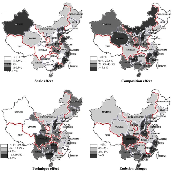
Figure 1. Divisia Decomposition results
(Annual average percentage changes)
The general positive numbers associated with the composition effect reveals the second pollution-increasing factor for most of Chinese provinces—a not surprising finding for a country in its early phase of industrialization process. There are only three exceptions, Beijing, Tianjin and Hubei, whose total composition effect appeared to be emission-reducing factor and also several other provinces whose total contribution from composition effect to emission increase is relatively small (below 2% per year), such as Shangdong, Jiangsu, Shanghai, Liaoning and Hebei. A common point between these provinces are their geographical location: they are all located in the east coast of China and their prosperous economic growth are all benefiting from high degree of commercial and capital openness. We suspect the
Technique effect <-14.110.5% -14.10.15% - -13.69.5% - 13.69.5% - -13.28.5% >-8.5%14.1% Emission changes <0% 0%-2% 2%-4% >4% Scale effect <138.5% 138.5%-159.5% 159.5%-1810.5% Composition effect <01% 01%-22.5% 22.5%-43.5% >43.5%
emission reduction contribution from composition effect in these five provinces is actually due to their participation into global production division system, in which, China, abundantly endowed with cheap labor forces, possesses actually comparative advantages in the relatively less polluting industries as textile, electronic equipment, etc. This idea can be better represented by the panel of composition effect in Figure 1, in which the pollution increase caused by composition effect is gradually reinforced when we move from east costal provinces to those located in the central and west China, especially for these northern provinces.
The regional disparity in the contribution of technique effect in emission evolves almost in the same proportion as that of scale effect. Except that this time, we observe a factor contributing to the reduction of emission. From Figure 1, we can see that it is the richer coastal provinces generally possess a higher technique effect. This result actually confirms our intuition that the technique effect increases with the income growth.
Adding up the three decomposed effects gives us the final emission variations. Clearly, the variation of the emission finally observed in the reality is actually a specific result for each province, whose formation actually depends closely on the characteristics of each province in the aspects of production scale, economic structure and technical progress. Looking carefully the six provinces whose annual average emission variation surpasses 4% in Figure 1, for the three provinces located in coastal area, Zhejiang, Fujian and Guangdong, their pollution situation is actually due to the fact that their strong expansion of industrial scale cancel out totally the emission reducing contribution from the technique effect. While for the 3 inland provinces, Sichuan, Shanxi and Henan, their emission increase is owing to the stronger pollution increasing contribution from composition transformation with respect to their relatively weaker technique capacity.
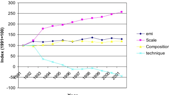
Figure 2 plots the detailed annual dynamic evolution of the national level industrial SO2 emission and its three contribution factors. Similar to the conclusion in Selden et al. (1999) and Bruvoll and Medin (2001), our decomposition results also emphasize the technique effect as the most important SO2 emission reducing factor. However, as there exists a mutual cancellation effect between scale effect which creates emission and technique effect that reduces the emission, it is actually the composition effect, whose contribution in emission stays relatively small and the result of the mutual cancellation between scale and composition effect that determine the final variation of the industrial SO2 emission.
Figure 2. Decomposition results on national level (1991-2001)
5. Tracing the trade-related scale, composition and technique effect—an empirical analysis based on the Divisia decomposition results
With the decomposed results of the contribution of scale, composition and technique effects in the total industrial SO2 emission, we can now check how international trade affect the final emission results in China.
5.1. Normalization of the variation index into the actual emission changes in quantity From eq. (15), we saw the Divisia index decomposition methods actually reasons on percentage change basis with reference to the original industrial emission level. Its contribution is to decompose the percentage change in industrial SO2 emission, ln(SO2it, SO2,i0) , into the contribution from scale enlargement ln(YYiit0), composition transformation
(
)
)] S S ln( ) w -w α w ( [ 1 -jit jit 1 -jit jit jit T 1 t n 1 j × + = =∑∑
and technique progress ln(eeiit0)+(
w -w)
) ln(II )] α w ( [ -1 jt jt -1 jit jit jit T 1 t n 1 j + × = = ∑ ∑ .However, our econometrical analysis actually requires the scale, composition and technique effect to be expressed in quantity of emission changes instead of the percentage changes. Therefore, as the first step, we need to normalize the decomposition results for the three effects. The normalization process is illustrated in equation (16)-(18). In this step, we simply use the total SO2 emission variation in each year with respect to the reference original
Figure 4.2. Decomposition result on national level (1991-2001)
-100 -50 0 50 100 150 200 250 300 1991 1992 1993 1994 1995 1996 1997 1998 1999 2000 2001 Year In d e x ( 1 9 9 1 = 1 0 0 ) emi Scale Composition technique
year 0 as the base value and attribute this value to the three effects according to their contribution shares. ) SO -SO ( ) SO / SO ln( ) Y Y ln( SO Δ 2 it, 2 i,0 0 ,i 2 t, i 2 0 ,i t, i scale ,t ,i , 2 = × (16)
(
)
) SO -SO ( ) SO / SO ln( )] S S ln( ) w -w α w ( [ SO Δ 2it, 2i,0 0 ,i 2 t, i 2 -1 jit jit -1 jit jit jit T 1 t n 1 j n compositio ,t ,i , 2 × × + = = = ∑ ∑ (17)(
)
) SO -SO ( ) SO / SO ln( )] I I ln( ) w -w α w ( [ ) ee ln( SO Δ 2 it, 2 i,0 0 ,i 2 t, i 2 -1 jt jt -1 jit jit jit T 1 t n 1 j i0 it technique ,t ,i , 2 × × + + = = = ∑ ∑ (18)5.2. Econometrical strategy and estimation results
Our empirical strategy in this section is relatively simple. As the variations in industrial SO2 emission related to international trade can be considered as a final combination of the three partial changes caused by scale, composition and technique effects, the objective of this section is to trace the indirect environmental role of trade through its separate impacts on the emission variations that are contributed by scale enlargement, composition transformation and technical progress.
Our investigation is carried out in two steps. In the first step, we regress the reduced-form estimation function, which relates trade intensity ratio directly to each of the three partial emission changes. In the second step, we regress the partial emission changes directly on their corresponding effects, measured respectively by industrial GDP, capital/labor abundance ratio and per capita GDP, by the Two Stage Least Square (2SLS) estimator. In this step, trade’s impact on emission via the three effects is actually captured by the first stage of the 2SLS estimation, in which we use trade liberalization degree as instruments for the scale, composition and technique effects. Although in the second step, the three effects are not the endogenous variables with respect to their corresponding emission changes, the 2SLS estimator actually enables us to separately analyze the impact of trade on the scale, composition and technique effect and how the three effects, in their turns, affect the total
emission results. Multiplying the coefficients of the structural determinants obtained in the second-stage 2SLS estimation with the trade’s coefficient found by the first stage instrumentation estimation, we can give a more direct description on how the trade intensity variation affects emission through each of the three channels.
Detailed reduced-form estimation results for the three effects are reported in table 2, 3 and 4. Tables 5-8 list the 2SLS structural estimation results.
As a general character often observed in Asian countries’ industrialization histories is that they often use foreign exchanges obtained from export to finance the import of machinery and equipment that used to support the development of some strategic heavy industries. If their export growth is stimulated by the demand from the world market, their import activity is more policy-oriented. Considering the possible difference in the role of export and import in economy and pollution, in the estimation carried out in this section, besides the (X+M)/GDP, we also check the emission determination role of export and import separately.4
We firstly include the export and import intensity (X/GDP and M/GDP) separately in the emission determination model B. Suspecting it might be the stock of the imported equipment and machinery instead of the annual import flow that has the capacity to affect the economic structure in China, we further replace in model C the import intensity (M/GDP) by the variable Mstock, which measures the employment of the stock of the imported equipment and machinery in total economy.5 This openness measurement is inspired by the CGE
production model of de Melo and Robinson (1990), in which the positive externality of the international trade on developing economy is describe through both the increasing export activities and the accumulation of the stock of imported machinery and equipment that increases the total effective capital.
These simple reduced-form estimations provide us with some reasonable results. Corresponding to the econometrical analysis in the previous sections, the reduced-form estimation model confirms that international trade (both export and import) generally plays emission-increasing role through scale effect but emission decreasing role via composition
4Agras and Chapman (1999) did the same arrangement in their paper.
5 Due to data unavailability, we use the stock of imported manufacture goods as an approximation for the stock of
imported equipment and machinery goods. This data series is compiled by author according to the provincial level statistical report in Almanac of China's Foreign Economic Relationship and Trade (1984-2001). We consider the stock of imported manufacture goods as a good approximation of the stock of imported equipments and machinery due to two reasons. Firstly, many of the imported manufacture goods in China are desitinated to re-export after being assembled. This type of imports is obviously helpful in increasing the productivity of Chinese industries. Secondly, the manufactured goods importation and the equipment and machinery importation data on the national level data are available since 1985, comparing these two series of data shows that the imports of the equipment and machinery occupied a very important and table percentage in total manufacture good import (over 50%). A simple correlation test between these two series also test reveals very strong correlation between these two data series by a coefficient of 0.9985.
and technique effects. However, a common point among the three tables of reduced-form estimation results is the unsatisfactory significance for all the three sets of trade intensity measures. This actually reminds us the underlying complexity of the trade-emission relationship.
Table 5-8 report the indirect environmental role of international trade on emission going through its three structural determinants. In the six columns related to 2SLS structural model, we separately use the three trade intensity measures as instruments for scale effect. The first-stage instrumentation estimation results are reported in the bottom of the table.
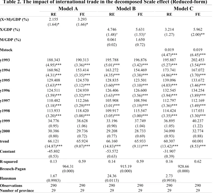
Table 2. The impact of international trade in the decomposed Scale effect (Reduced-form)
Model A Model B Model C
RE FE RE FE RE FE (X+M)/GDP (%) 2.155 3.293 (1.64)* (1.66)* X/GDP (%) 4.746 5.631 3.214 5.962 (1.48)° (1.53)° (1.27) (2.00)** M/GDP (%) 0.061 1.650 (0.02) (0.72) Mstock 0.019 0.019 (4.47)*** (6.45)*** y1993 188.343 190.313 195.788 196.876 195.887 202.453 (4.95)*** (3.36)*** (5.01)*** (3.42)*** (5.27)*** (3.54)*** y1994 160.962 153.414 163.272 154.469 173.741 167.072 (4.31)*** (3.35)*** (4.35)*** (3.38)*** (4.86)*** (3.70)*** y1995 129.408 124.570 128.835 123.501 139.096 133.672 (3.63)*** (3.12)*** (3.60)*** (3.10)*** (4.03)*** (3.46)*** y1996 124.511 124.939 126.406 126.600 132.545 134.254 (3.59)*** (3.52)*** (3.63)*** (3.56)*** (3.94)*** (3.89)*** y1997 110.482 112.266 105.908 108.594 112.797 112.169 (3.18)*** (3.29)*** (3.01)*** (3.19)*** (3.36)*** (3.49)*** y1998 113.933 118.420 109.917 115.547 114.424 117.031 (3.20)*** (3.08)*** (3.05)*** (3.00)*** (3.35)*** (3.30)*** y1999 34.776 38.628 33.196 37.749 36.895 40.237 (0.95) (1.06) (0.90) (1.04) (1.05) (1.22) y2000 30.386 29.736 29.208 28.733 34.090 32.774 (0.80) (0.72) (0.77) (0.69) (0.93) (0.88) trend 66.121 65.924 66.160 65.933 60.307 60.001 (14.87)*** (9.07)*** (14.83)*** (9.11)*** (13.42)*** (8.53)*** Constant -45.802 -53.572 -31.907 (0.53) (0.63) (0.39) R-squared 0.13 0.59 0.14 0.59 0.16 0.62 Breusch-Pagan (0.000)964.31 (0.000)915.19 (0.000)928.66 Hausman (0.9983)1.67 (0.0113)24.36 (0.9938)2.73 Observations 290 290 290 290 290 290 Number of province 29 29 29 29 29 29
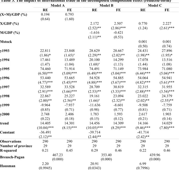
Table 3. The impact of international trade in the decomposed composition effect (reduced-form)6
Model A Model B Model C
RE FE RE FE RE FE (X+M)/GDP (%) 0.194 0.793 (0.64) (1.60) X/GDP (%) 2.172 2.507 0.770 2.227 (2.52)** (2.86)*** (1.24) (2.61)*** M/GDP (%) -1.616 -0.421 (2.11)** (0.53) Mstock 0.001 0.001 (0.50) (0.74) y1993 22.811 23.848 28.629 28.667 24.431 27.896 (1.86)* (1.65)° (2.29)** (2.02)** (1.98)** (1.95)* y1994 17.461 13.489 20.100 14.299 17.078 13.516 (1.47) (1.04) (1.68)° (1.13) (1.44) (1.08) y1995 74.460 71.914 74.491 71.149 73.984 71.080 (6.50)*** (5.09)*** (6.49)*** (5.04)*** (6.44)*** (5.04)*** y1996 53.440 53.665 54.928 54.885 54.064 54.941 (4.77)*** (5.45)*** (4.88)*** (5.67)*** (4.82)*** (5.61)*** y1997 32.589 33.528 28.709 30.819 32.315 31.955 (2.91)*** (3.66)*** (2.53)** (3.33)*** (2.88)*** (3.54)*** y1998 22.867 25.227 19.161 23.094 23.022 24.379 (2.00)** (2.56)** (1.66)° (2.32)** (2.02)** (2.55)** y1999 -9.964 -7.937 -11.636 -8.601 -9.508 -7.759 (0.85) (0.71) (0.98) (0.77) (0.81) (0.71) y2000 2.748 2.406 1.783 1.593 2.617 1.903 (0.22) (0.18) (0.15) (0.12) (0.21) (0.14) trend 14.405 14.301 14.456 14.309 14.166 14.029 (10.04)*** (8.15)*** (10.05)*** (8.29)*** (9.46)*** (7.80)*** Constant -36.491 -39.714 -41.714 (2.12)** (2.44)** (2.42)** Observations 290 290 290 290 290 290 Number of province 29 29 29 29 29 29 R-squared 0.21 0.45 0.29 0.46 0.22 0.46 Breusch-Pagan (0.000)467.23 (0.000)353.40 (0.000)439.96 Hausman (0.9945)2.20 (0.0343)20.91 (0.7996)6.99
Absolute value of z statistics in parentheses, ° significant at 15%, * significant 10%, ** significant 5%, *** significant 1%.
6 For the aim of correspondence to the empirical analyses in chapter 4, in the appendix of this chapter, we report
both the reduced-form and 2SLS estimation results for the decomposed composition effect without time trend and time-specific effects.
Table 4. The impact of international trade in the decomposed technique effect (reduced-form)
Model A Model B Model C
RE FE RE FE RE FE (X+M)/GDP (%) -2.594 -4.129 (2.17)** (2.26)** X/GDP (%) -6.141 -7.750 -4.792 -8.261 (2.08)** (2.38)** (2.05)** (2.74)*** M/GDP (%) 0.322 -1.564 (0.13) (0.73) Mstock -0.012 -0.012 (3.01)*** (4.85)*** y1993 -205.196 -207.855 -215.421 -218.031 -214.369 -222.667 (5.81)*** (3.82)*** (5.95)*** (3.99)*** (6.09)*** (4.08)*** y1994 -163.827 -153.643 -167.189 -155.367 -173.280 -164.880 (4.72)*** (3.43)*** (4.80)*** (3.50)*** (5.11)*** (3.73)*** y1995 -178.305 -171.777 -177.626 -170.170 -184.125 -177.299 (5.38)*** (4.54)*** (5.35)*** (4.51)*** (5.63)*** (4.78)*** y1996 -178.315 -178.892 -180.918 -181.468 -184.528 -186.704 (5.53)*** (5.18)*** (5.59)*** (5.30)*** (5.79)*** (5.50)*** y1997 -151.691 -154.099 -145.340 -148.373 -150.506 -149.732 (4.70)*** (4.72)*** (4.45)*** (4.50)*** (4.73)*** (4.73)*** y1998 -75.298 -81.352 -69.654 -76.838 -73.276 -76.584 (2.28)** (2.63)*** (2.09)** (2.47)** (2.26)** (2.64)*** y1999 -20.531 -25.729 -18.262 -24.320 -20.979 -25.214 (0.60) (0.80) (0.54) (0.76) (0.63) (0.83) y2000 5.934 6.812 7.564 8.410 4.292 5.941 (0.17) (0.17) (0.21) (0.21) (0.12) (0.16) trend -70.189 -69.923 -70.247 -69.940 -66.510 -66.107 (16.99)*** (10.12)*** (16.97)*** (10.19)*** (15.62)*** (9.63)*** Constant 105.935 115.963 101.800 (1.39) (1.54) (1.38) Observations 290 290 290 290 290 290 Number of provcode 29 29 29 29 29 29 R-squared 0.15 0.64 0.17 0.65 0.17 0.65 Breusch-Pagan (0.000)927.80 (0.000)873.65 (0.000)875.98 Hausman (0.9437)4.08 (0.6961)8.19 (0.9551)4.44
Table 5. Trade’s impact on industrial SO2 emission—Channel 1: enlargement of the
industrial production scale
Simple Model A Model B2SLS Model C
RE FE RE FE RE FE RE FE Ind. GDP 0.481 0.480 0.421 0.595 0.268 0.350 0.280 0.296 (16.69)*** (8.52)*** (2.59)*** (1.66)* (2.34)** (1.72)* (6.13)*** (6.22)*** y1993 186.420 186.415 186.192 186.848 185.619 185.926 185.663 185.725 (6.87)*** (4.36)*** (6.99)*** (3.32)*** (6.34)*** (3.33)*** (6.36)*** (3.34)*** y1994 176.830 176.825 176.632 177.201 176.134 176.401 176.173 176.226 (6.80)*** (4.94)*** (6.92)*** (3.68)*** (6.28)*** (3.69)*** (6.30)*** (3.80)*** y1995 144.485 144.467 143.740 145.882 141.868 142.870 142.012 142.213 (5.73)*** (4.77)*** (5.79)*** (3.48)*** (5.21)*** (3.48)*** (5.24)*** (3.59)*** y1996 132.457 132.429 131.353 134.526 128.580 130.065 128.794 129.091 (5.34)*** (4.99)*** (5.36)*** (3.62)*** (4.79)*** (3.63)*** (4.83)*** (3.77)*** y1997 116.792 116.762 115.570 119.082 112.502 114.145 112.738 113.067 (4.71)*** (4.66)*** (4.71)*** (3.37)*** (4.19)*** (3.32)*** (4.23)*** (3.50)*** y1998 117.905 117.865 116.332 120.851 112.384 114.498 112.687 113.111 (4.67)*** (4.34)*** (4.64)*** (3.10)*** (4.11)*** (3.05)*** (4.15)*** (3.21)*** y1999 42.062 42.016 40.223 45.508 35.606 38.079 35.961 36.457 (1.62)° (1.85)* (1.55)° (1.21) (1.26) (1.06) (1.29) (1.12) y2000 40.271 40.244 39.180 42.316 36.441 37.908 36.651 36.945 (1.48)° (1.73)* (1.46) (0.99) (1.24) (0.90) (1.26) (0.99) trend 28.169 28.290 33.003 19.115 45.137 38.639 44.204 42.901 (7.19)*** (5.94)*** (2.48)** (0.68) (4.64)*** (2.33)** (8.87)*** (5.66)*** Constant -103.628 -103.267 -89.187 -130.678 -52.938 -72.350 -55.724 (1.93)* (1.84)* (1.07) (1.12) (0.74) (0.84) (0.89) Obs. 290 290 290 290 290 290 290 290 Group # 29 29 29 29 29 29 29 29 R-squared 0.79 0.60 0.60 0.56 0.59 0.56 0.57 Breusch-Pagan (0.000)934.48 Hausman 0.02 (1.000) Iden. test (1.000)0.014 (1.000)0.030 (0.9599)3.70 (0.9999)0.94 (0.0003)***32.24 (0.0036)***26.10
Trade elasticity of decomposed emission changes caused by industrial production scale enlargement
(X+M)/GDP 0.152 0.193
X/GDP 0.164 0.194 0.104 0.123
M/GDP -0.035 -0.039
Mstock 0.060 0.064
First-stage coefficient for the international trade instruments (on ind. GDPjt)
(X+M)/GDP (%) 6.160 5.534 (3.05)*** (1.36) X/GDP (%) 20.580 18.669 11.897 14.056 (4.48)*** (2.04)** (4.20)*** (3.23)*** M/GDP (%) -4.536 -3.808 (1.21) (0.68) Mstock 0.067 0.067 (14.41)*** (16.14)*** The detailed calculation equation for elasticity of export intensity ratio for decomposed scale effect is as following, d(dscale(X/GDPeffect))=
= × × × 2 SO GDP . ind 296 . 0 GDP . ind GDP / X 056 . 14 0.123 SO GDP / X 296 . 0 096 . 14 2 = ×
× . Here 14.096 and 0.296 are the coefficients obtained for export intensity in the instrumentation estimation and for industrial GDP in the second-stage fixed-effect estimation result of model C, respectively. The X/GDP,ind.GDP and SO2mean the sample average value of X/GDP, industrial GDP and the decomposed industrial SO2
emission variation related to the scale effect. The elasticity of trade for the other two decomposed emission changes is calculated in the same way.
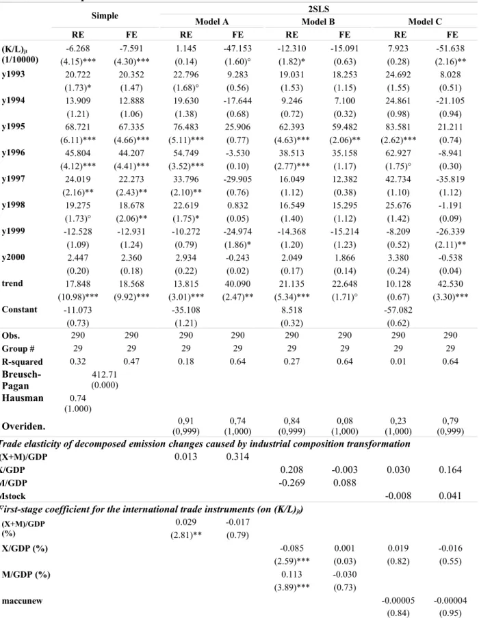
Table 6. Trade’s impact on industrial SO2 emission—Channel 2: transformation of
industrial composition
Simple Model A Model B2SLS Model C
RE FE RE FE RE FE RE FE (K/L)jt (1/10000) -6.268 -7.591 1.145 -47.153 -12.310 -15.091 7.923 -51.638 (4.15)*** (4.30)*** (0.14) (1.60)° (1.82)* (0.63) (0.28) (2.16)** y1993 20.722 20.352 22.796 9.283 19.031 18.253 24.692 8.028 (1.73)* (1.47) (1.68)° (0.56) (1.53) (1.15) (1.55) (0.51) y1994 13.909 12.888 19.630 -17.644 9.246 7.100 24.861 -21.105 (1.21) (1.06) (1.38) (0.68) (0.72) (0.32) (0.98) (0.94) y1995 68.721 67.335 76.483 25.906 62.393 59.482 83.581 21.211 (6.11)*** (4.66)*** (5.11)*** (0.77) (4.63)*** (2.06)** (2.62)*** (0.74) y1996 45.804 44.207 54.749 -3.530 38.513 35.158 62.927 -8.941 (4.12)*** (4.41)*** (3.52)*** (0.10) (2.77)*** (1.17) (1.75)° (0.30) y1997 24.019 22.273 33.796 -29.905 16.049 12.382 42.734 -35.819 (2.16)** (2.43)** (2.10)** (0.76) (1.12) (0.38) (1.10) (1.12) y1998 19.275 18.678 22.619 0.832 16.549 15.295 25.676 -1.191 (1.73)° (2.06)** (1.75)* (0.05) (1.40) (1.12) (1.42) (0.09) y1999 -12.528 -12.931 -10.272 -24.974 -14.368 -15.214 -8.209 -26.339 (1.09) (1.24) (0.79) (1.86)* (1.20) (1.23) (0.52) (2.11)** y2000 2.447 2.360 2.934 -0.243 2.049 1.866 3.380 -0.538 (0.20) (0.18) (0.22) (0.02) (0.17) (0.14) (0.24) (0.04) trend 17.848 18.568 13.815 40.090 21.135 22.648 10.128 42.530 (10.98)*** (9.92)*** (3.01)*** (2.47)** (5.34)*** (1.71)° (0.67) (3.30)*** Constant -11.073 -35.108 8.518 -57.082 (0.73) (1.21) (0.32) (0.62) Obs. 290 290 290 290 290 290 290 290 Group # 29 29 29 29 29 29 29 29 R-squared 0.32 0.47 0.18 0.64 0.27 0.64 0.01 0.64 Breusch-Pagan 412.71 (0.000) Hausman 0.74 (1.000) Overiden. (0,999)0,91 (1,000)0,74 (0,999)0,84 (1,000)0,08 (1,000)0,23 (0,999)0,79
Trade elasticity of decomposed emission changes caused by industrial composition transformation
(X+M)/GDP 0.013 0.314
X/GDP 0.208 -0.003 0.030 0.164
M/GDP -0.269 0.088
Mstock -0.008 0.041
First-stage coefficient for the international trade instruments (on (K/L)jt)
(X+M)/GDP (%) 0.029 -0.017 (2.81)** (0.79) X/GDP (%) -0.085 0.001 0.019 -0.016 (2.59)*** (0.03) (0.82) (0.55) M/GDP (%) 0.113 -0.030 (3.89)*** (0.73) maccunew -0.00005 -0.00004 (0.84) (0.95) Absolute value of z statistics in parentheses, ° significant at 15%, * significant 10%, ** significant 5%, *** significant 1%.
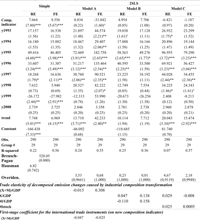
Table 7. Trade’s impact on industrial SO2 emission—Channel 2: transformation of
industrial composition (New composition indicator)
Simple Model A Model B2SLS Model C
RE FE RE FE RE FE RE FE Comp. indicator 7.664 8.556 0.834 -31.842 4.954 7.706 -6.421 -1.187 (7.80)*** (5.67)*** (0.22) (1.60)° (0.85) (1.08) (0.97) (0.20) y1993 17.157 16.538 21.897 44.574 19.038 17.128 26.932 23.299 (1.56) (1.22) (1.48) (2.21)** (1.61)° (1.11) (1.75)* (1.52) y1994 16.180 15.882 18.467 29.407 17.088 16.166 20.896 19.144 (1.53) (1.35) (1.32) (2.06)** (1.58) (1.25) (1.47) (1.49) y1995 49.416 46.405 72.469 182.758 58.563 49.276 96.955 79.290 (4.60)*** (3.98)*** (3.91)*** (2.65)*** (2.65)*** (1.77)* (3.72)*** (3.23)*** y1996 33.607 31.307 51.217 135.464 40.595 33.500 69.921 56.427 (3.24)*** (3.49)*** (3.12)*** (2.54)** (2.25)** (1.59) (3.23)*** (3.04)*** y1997 18.268 16.636 30.760 90.521 23.225 18.192 44.028 34.455 (1.79)* (2.11)** (2.06)** (2.35)** (1.58) (1.11) (2.44)** (2.36)** y1998 7.632 5.948 20.527 82.222 12.749 7.554 34.225 24.343 (0.73) (0.69) (1.35) (2.07)* (0.85) (0.44) (1.86)* (1.61)° y1999 -26.172 -27.982 -12.313 53.990 -20.673 -26.256 2.408 -8.213 (2.44)** (2.91)*** (0.78) (1.26) (1.30) (1.38) (0.12) (0.50) y2000 2.739 2.725 2.846 3.358 2.781 2.738 2.960 2.878 (0.25) (0.25) (0.20) (0.25) (0.25) (0.20) (0.20) (0.21) trend 7.748 6.969 13.710 42.233 10.114 7.712 20.043 15.474 (5.01)*** (4.15)*** (3.71)*** (2.40)** (1.94) (1.19) (3.34)*** (2.92)*** Constant -166.438 -46.092 -118.685 81.740 (7.33)*** (0.68) (1.15) (0.70) Obs. 290 290 290 290 290 290 290 290 Group # 29 29 29 29 29 29 29 29 R-squared 0.22 0.56 0.24 0.55 0.25 0.56 0.07 0.57 Breusch-Pagan 528.05 (0.000) Hausman 6.82 (0.742) Overiden. (0,9661)3,53 (1,000)0,68 (1,000)0,23 (1,000)0,01 (0,9119)4,67 (0,9948)2,18
Trade elasticity of decomposed emission changes caused by industrial composition transformation
(X+M)/GDP -0.015 0.308
X/GDP 0.047 0.138 0.029 -0.008
M/GDP -0.110 0.158
Mstock 0.025 0.0005
First-stage coefficient for the international trade instruments (on new composition indicator)
(X+M)/GDP (%) -0.047 -0.025 (4.52)*** (0.69) X/GDP (%) 0.048 0.090 -0.023 0.034 (0.96) (1.42) (0.693) (0.72) M/GDP (%) -0.113 0.106 (2.62)*** (1.94)* maccunew -0.0002 -0.0002 (2.87)*** (3.40)*** Absolute value of z statistics in parentheses, ° significant at 15%, * significant 10%, ** significant 5%, *** significant 1%. Detailed introduction for the new composition indicator is available in appendix of this chapter.
Table 8. Trade’s impact on industrial SO2 emission—Channel 3: technique progress
Simple Model A Model B2SLS Model C
RE FE RE FE RE FE RE FE (GDPPC)jt (1/1000) -248.380 -438.174 -56.935 -121.885 -62.193 -125.118 -81.423 -103.787 (3.64)*** (3.15)*** (2.04)** (2.26)** (2.25)** (2.39)** (3.70)*** (4.43)*** (GDPPC)jt2 (1/1000)2 19.680 36.014 (2.59)*** (2.91)*** (GDPPC)jt3 (1/1000)3 -0.547 -1.069 (1.90)* (2.69)*** y1993 -190.633 -183.624 -201.451 -202.302 -201.519 -202.344 -201.771 -202.065 (5.56)*** (3.74)*** (5.58)*** (3.75)*** (5.56)*** (3.78)*** (5.48)*** (3.79)*** y1994 -163.845 -152.055 -181.896 -182.881 -181.976 -182.930 -182.267 -182.607 (4.95)*** (3.71)*** (5.26)*** (3.94)*** (5.24)*** (3.94)*** (5.17)*** (4.05)*** y1995 -169.593 -156.267 -190.346 -191.499 -190.439 -191.557 -190.781 -191.178 (5.27)*** (4.58)*** (5.68)*** (4.94)*** (5.66)*** (4.96)*** (5.58)*** (5.06)*** y1996 -155.992 -141.582 -178.013 -178.783 -178.076 -178.821 -178.303 -178.568 (4.92)*** (4.52)*** (5.40)*** (5.18)*** (5.38)*** (5.23)*** (5.30)*** (5.30)*** y1997 -126.321 -111.637 -147.182 -146.678 -147.141 -146.653 -146.992 -146.819 (3.98)*** (3.68)*** (4.46)*** (4.57)*** (4.44)*** (4.58)*** (4.37)*** (4.63)*** y1998 -46.997 -34.025 -63.941 -62.654 -63.837 -62.589 -63.456 -63.012 (1.46) (1.21) (1.91)* (2.13)** (1.90)* (2.14)** (1.86)* (2.19)** y1999 -3.015 2.166 -15.181 -19.096 -15.498 -19.291 -16.657 -18.005 (0.09) (0.07) (0.44) (0.60) (0.45) (0.61) (0.47) (0.59) y2000 5.560 4.183 -4.796 -15.345 -5.650 -15.870 -8.773 -12.406 (0.16) (0.11) (0.13) (0.38) (0.15) (0.39) (0.24) (0.32) trend -35.531 -9.297 -51.677 -30.047 -49.926 -28.970 -43.522 -36.074 (4.01)*** (0.54) (5.07)*** (1.71)* (4.93)*** (1.69)° (5.12)*** (3.79)*** Constant 446.931 148.596 158.835 196.278 (3.53)*** (1.74)* (1.86)* (2.39)** Obs. 290 290 290 290 290 290 290 290 Group # 29 29 29 29 29 29 29 29 R-squared 0.12 0.67 0.13 0.73 0.12 0.73 0.09 0.79 Breusch-Pagan (0.000)891.11 Hausman 13.85 (0.3103) Overiden. (0,9986)1,59 (0,9501)3,94 (0,9945)2,21 (0,9057)4,77 (0,5014)9,33 (0,3853)10,65
Trade elasticity of decomposed emission changes caused by technical progress
(X+M)/PIB -0.145 -0.253
X/GDP -0.117 -0.228 -0.173 -0.205
M/GDP -0.051 -0.060
Mstock -0.025 -0.032
First-stage coefficient for the international trade instruments (on GDPPCjt)
(X+M)/GDP (%) 0.042 0.034 (8.06)*** (3.09)*** X/GDP (%) 0.061 0.059 0.069 0.064 (4.61)*** (3.04)*** (7.04)*** (3.74)*** M/GDP (%) 0.027 0.016 (2.48)** (1.20) Mstock 0.0001 0.0001 (7.87)*** (4.20)*** Absolute value of z statistics in parentheses, ° significant at 15%, * significant 10%, ** significant 5%, *** significant 1%.
Let’s first look at the results concerning the environmental role of trade through production scale enlargement impact in table 5. Good coherence between the results of the second-stage 2SLS estimation and those in the reduced-form model can be easily observed in this table. In two to three cases, the changes in the trade intensity measurement and estimation methods do not affect the coefficients of the trade variables. The only exception is the model B, where we only prove the significant positive coefficients for export intensity. As the Hausman specification test indicates the best instrumentation efficiency to be in Model C, in which we use X/GDP and Mstock/GDP to instrument industrial GDP. We believe this result actually confirms the assumption of the CGE model of de Melo and Robinson (1990) on its production function—the growth of domestic economy benefits the positive spillover effect from both the export intensity increase and the accumulation in the imported equipment and machinery. Therefore, we will base our following discussion on the result of model C. To sum up, the estimation results in both tables 2 and 5 generally confirm the positive causality between the trade intensity (either total trade intensity or annual export intensity and the stock of imported machinery and equipment), the industrial production scale, and the decomposed industrial emission variation related to scale effect. This conclusion is also expressed in the table 5 by the positive trade elasticity of the decomposed scale effect.
The estimations for the decomposed composition effect do not obtain such a good coherence. Most of the coefficients for the composition effect measure—capital/labor abundance ratio shows negative coefficients even after being instrumented by the trade intensity variables (c.f. fixed effect estimation results in table 6). This finding is actually contradictory with our intuition that suggests an industrial sectors using intensively capital in its production process generate equally more intensively pollution problems.
This contrary-to-intuition result may be due to the fact that the capital-abundance ratio, being a pertinent extrapolation for the composition effect when analysis focus covers the whole economy, may lose its pertinence when the analysis is concentrated only in the industrial sector. Here is our explanation. The pollution performance of whole economy structure and the total capital-abundance level may follow similar evolution trajectory when economy starts from less capital-intensive and less pollution-intensive agriculture-dominated structure, then experiences the industrialization procedures that leads both capital intensity and pollution intensity to increase and finally arrives the post-industry structure whose production process returns to be low capital-intensive and low pollution intensive style. However, once our attention is focused only in the industrial sectors, less polluting industries might not necessarily be the sectors possessing less capital abundance ratio, the example is the
information industries. Moreover, in the relatively early stage of industrialization procedure, though the less polluting light industries may generally possess relatively lower capital abundance ratio, for the enterprises in the same industry, higher capital abundance ratio may means better technology efficiency, therefore means less pollution problems. Dinda et al (2000) also indicate the potential ambiguity in using capital abundance as measurement for environmental performance of the industrial composition, since the “capital intensive sector could also be more likely to be clean technology owner”.
To overcome the ambiguity of this simple composition effect measurement, we make use of the detailed value added data of 13 industrial sectors in each province to construct a synthetic composition indicator for each provinces as following, I )
Y Y ( Ω ,j0 j it jit it=
∑
× . Yjit signifiesthe detailed value added in industrial sector j of province i at time t and Ij,0 is the initial national average SO2 emission intensity for each of the 13 sectors in year 1991.7 As the sum of value added of the 13 industrial sectors generally counts up to 98% of the total provincial industrial GDP each year, we are confident about the representative capability of this synthetic indicator as the measurement for the general environmental performance of the industrial composition.8
The 2SLS structural model estimation results based on this new composition effect measurement are listed in table 7. The new synthetic composition indicator does improve the reliability of the estimation results. The expected positive coefficients are firstly obtained by the simple estimations. However, for the structural models, most of these positive coefficients stay insignificant and the trade intensity variables also show low instrumentation efficiency. We therefore fail to capture significant impact of trade on emission through China’s industrial composition transformation.
The estimation results obtained for the decomposed emission variations related to technique effect are relatively more satisfactory (c.f. Table 8). As expected, per capita GDP is a pertinent approximation for the technique effect, especially when collectively instrumented by the trade intensity indicators X/GDP and Mstock. In this estimation result, the positive GDPPC coefficient shows the highest significance. The estimation proves an obvious environment-friendly role for international trade through technique effect. This conclusion is also revealed in Table 8 by the unanimous negative trade elasticity.
7 More discussion about the advantages and deficiencies of this synthetic composition effect measurement is
included in the appendix.
8 Keller and Levinson (2002) also use the same expression to measure industry composition of each state in order
6. Conclusion
In this paper, we introduced and adjusted the traditional Divisia index decomposition method and employed it to Chinese data. By deepening our analysis insight into the detailed 13 industrial sectors in each province, the Divisia decomposition method revealed more concrete contribution of industrial scale enlargement, composition transformation and technical progress in industrial SO2 emission changes for each province during 1991-2001.
The decomposition results reveals the contributions of the three structural determinants of emission in China’s industrial SO2 emission variation, it gives more structural explanation for the ever-increasing tendency in total industrial SO2 emission in China during the last decade. Besides the contribution from the rapid expansion in industrial production scale, we find that the industrial composition transformation process also plays as pollution-increasing factor in most of Chinese provinces. Only several coastal provinces whose industrialization largely benefited from their advantageous geographical location and openness policy have been the exceptions. Accompanying scale enlargement, the economic growth in each province also catalyzed the technique effect, a pollution-reducing factor. As expected, it is the ricer coastal provinces possess a technique effect relativement more important owing to their relatively higher income level.
Coherent to most of previous emission decomposition studies, our findings show the scale and technique effects as the two most important emission variation contributors, but in opposite directions. This actually leads the final changes in SO2 emission to be determined by the combination of the composition effect with the left impact from the mutual cancellation between scale and technique effect. However, when the analysis is précised to the special case of each province, the variation of its emission during the time is in fact a particular result, which is determined by the combination of its three specific structural characteristics.
The Divisia decomposition results also permit us to separately investigate the potential relationship between the trade intensity indicators and the three parts of emission variation caused scale enlargement, composition transformation and technical progress through both a reduced-form model and a structural model estimated by 2SLS method. This simple econometrical strategy clarified the relationship of trade with both scale and technique effects. We prove the significant role of the trade as a positive factor in production scale enlargement, and an active catalyst for the technological progress in pollution control activities but failed to derive a clear conclusion for the role of trade on China’s industrial composition transformation.