HAL Id: hal-01386617
https://hal.sorbonne-universite.fr/hal-01386617
Submitted on 24 Oct 2016
HAL is a multi-disciplinary open access archive for the deposit and dissemination of sci-entific research documents, whether they are pub-lished or not. The documents may come from teaching and research institutions in France or abroad, or from public or private research centers.
L’archive ouverte pluridisciplinaire HAL, est destinée au dépôt et à la diffusion de documents scientifiques de niveau recherche, publiés ou non, émanant des établissements d’enseignement et de recherche français ou étrangers, des laboratoires publics ou privés.
Kailiang Xu, Jean-Gabriel Minonzio, Dean Ta, Bo Hu, Weiqi Wang, Pascal
Laugier
To cite this version:
Kailiang Xu, Jean-Gabriel Minonzio, Dean Ta, Bo Hu, Weiqi Wang, et al.. Sparse SVD Method for High-Resolution Extraction of the Dispersion Curves of Ultrasonic Guided Waves. IEEE Transactions on Ultrasonics, Ferroelectrics and Frequency Control, Institute of Electrical and Electronics Engineers, 2016, 63 (10), pp.1514 - 1524. �10.1109/TUFFC.2016.2592688�. �hal-01386617�
For Review Only
1
Sparse SVD Method for High Resolution Extraction of the Dispersion Curves of Ultrasonic Guided 2
Waves 3
4
Kailiang Xu1,2, Jean-Gabriel Minonzio2, Dean Ta1,3,4, Bo Hu1, Weiqi Wang1, Pascal Laugier2 5
6
1 Department of Electronic Engineering Fudan University, Shanghai, China. 7
2 Sorbonne Universités, UPMC Univ Paris 06, CNRS, INSERM, Laboratoire d’Imagerie Biomédicale 8
(LIB), 75006, Paris, France. 9
3 State Key Laboratory of ASIC and System, Fudan University, Shanghai, China 10
4 Key Laboratory of Medical Imaging Computing and Computer Assisted Intervention (MICCAI) of 11
Shanghai, Shanghai, China 12
*Corresponding authors: E-mails: Kailiang Xu, xukl.fdu@gmail.com 13 14 2 3 4 5 6 7 8 9 10 11 12 13 14 15 16 17 18 19 20 21 22 23 24 25 26 27 28 29 30 31 32 33 34 35 36 37 38 39 40 41 42 43 44 45 46 47 48 49 50 51 52 53 54 55 56 57 58 59
For Review Only
Abstract —The two-dimensional Fourier transform (2D-FT) analysis of multichannel signals is a
1
straightforward method to extract the dispersion curves of guided modes. Basically, the time signals 2
recorded at several positions along the waveguide are converted to the wavenumber-frequency space, so 3
that the dispersion curves (i.e., the frequency-dependent wavenumbers) of the guided modes can be 4
extracted by detecting peaks of energy trajectories. In order to improve the dispersion curves extraction of 5
low amplitude modes propagating in cortical bone, a multi-emitter and multi-receiver transducer array has 6
been developed together with an effective singular vector decomposition (SVD) based signal processing 7
method. However, in practice, the limited number of positions where these signals are recorded results in 8
a much lower resolution on the wavenumber axis than on the frequency axis. This prevents a clear 9
identification of overlapping dispersion curves. In this study, a sparse SVD (S-SVD) method, which 10
combines the SNR improvement of the SVD-based approach with the high wavenumber resolution 11
advantage of the sparse optimization, is presented to overcome the above mentioned limitation. Different 12
penalty constraints, i.e., 𝑙1-norm, Frobenius norm and revised Cauchy norm, are compared with the sparse
13
characteristics. The regularization parameters are investigated with respect to the convergence property and 14
wavenumber resolution. The proposed S-SVD method is investigated using synthetic wideband signals, 15
experimental data obtained from a bone-mimicking phantom and from an ex-vivo human radius. The 16
analysis of the results suggests that the S-SVD method has the potential to significantly enhance the 17
wavenumber resolution and to improve the extraction of the dispersion curves. 18 19 2 3 4 5 6 7 8 9 10 11 12 13 14 15 16 17 18 19 20 21 22 23 24 25 26 27 28 29 30 31 32 33 34 35 36 37 38 39 40 41 42 43 44 45 46 47 48 49 50 51 52 53 54 55 56 57 58 59 60
For Review Only
I. INTRODUCTION 1
The dispersion characteristics of elastic guided waves have attracted considerable attention and brought out 2
many useful applications, such as seismic waves analysis [1-6], underwater acoustics [7-9], non-destructive 3
evaluation [10-13] and biomedical applications [14-17]. Following the different implementations of signal 4
recording, the dispersion characteristics extraction methods can mainly be classified into two categories, 5
i.e., single-channel processing [7-9, 11, 14] and multichannel processing [4, 10, 15, 18-20]. 6
Regarding the single-channel processing, the time-frequency representation (TFR) method enables the 7
computation of the dispersive energy simultaneously in time and frequency [21]. In 1999, Prosser et al. [11]
8
applied the TFR method to characterize Lamb modes dispersion. Several TFR-based dispersion curves 9
extraction strategies have been proposed. For example, aiming to overcome the TFR uncertainty principle 10
(which actually determines that there is an inherent trade-off between the time and frequency resolution in 11
the spectrogram) and to enhance the mode extraction capabilities, some improved TFR methods have been 12
proposed in which the signals are decomposed into TFR atoms whose group delays are nonlinearly 13
modulated in frequency and determined with respect to the local wave dispersion, such as the group delay 14
shift covariant quadratic TFR [7], warped TFR method [22], Chirplet transform [23], generalized warblet 15
transform based TFR method [24] and dispersion-based TFR method [25]. Recently, Xu et al. [26] have 16
employed the dispersion compensation technique [27, 28] for multimode separation. In underwater 17
acoustics field, Bonnel et al. [9] successfully utilized the robust physical a priori information of the oceanic 18
waveguide to separate some overlapped modes, which was difficult with the classical TFR methods. Those 19
refined dispersion mode extraction methods were basically implemented based on artificially 20 2 3 4 5 6 7 8 9 10 11 12 13 14 15 16 17 18 19 20 21 22 23 24 25 26 27 28 29 30 31 32 33 34 35 36 37 38 39 40 41 42 43 44 45 46 47 48 49 50 51 52 53 54 55 56 57 58 59
For Review Only
shifting/compensating the mode energy distribution by considering that the dispersion characteristics can 1
be well determined by the modal theory. Since their performances rely on the a priori knowledge of the 2
waveguide characteristics, further improvements are still required. An iterative estimation method has been 3
designed with the dispersion-based TFR analysis whose tilling is determined with respect to the dispersion 4
curves extracted from the TFR ridges [25]. However, due to the limited information recorded by the single-5
channel measurement, the extraction of the dispersion characteristics of low-amplitude modes remains 6
challenging, especially for the accurate evaluation of complex medium, such as human long cortical bones 7
[19, 29]. 8
Improvement of the separation of multiple propagation modes superimposed and interfered in the time 9
domain can be achieved using the multichannel recording method combined with some appropriate 10
multichannel data processing techniques [2-4, 20]. Among them, the most straightforward approach is to 11
map the data from time-distance to the frequency-wavenumber space using the spatio-temporal two-12
dimensional Fourier transform (2-D FT) [1, 2, 10]. In practice, whereas the relatively long duration of the 13
recorded time signals ensures a high frequency resolution, the limited number of positions where these 14
signals are recorded with a finite receiving aperture still results in a low resolution on the wavenumber axis. 15
Recently, Harley et al. [40] applied compressed sensing to process single-emitter multi-receiver ultrasonic
16
signals for sparse wavenumber extraction of Lamb modes. Actually, since the 1980s, the sparse inversion 17
techniques have been developed in seismic data analysis to overcome the consequence of limited aperture 18
and discretization and to improve the wavenumber resolution [30]. In 1985, Thorson and Claerbout [31]
19
originally proposed the least-squares stochastic inversion, which allows better noise filtering and velocity 20 2 3 4 5 6 7 8 9 10 11 12 13 14 15 16 17 18 19 20 21 22 23 24 25 26 27 28 29 30 31 32 33 34 35 36 37 38 39 40 41 42 43 44 45 46 47 48 49 50 51 52 53 54 55 56 57 58 59 60
For Review Only
and offset space reconstruction in the Radon domain. Sacchi and Ulrych [32] improved the method with an 1
appealing alternative solution based on sparse inversion, called high-resolution Radon transform, which 2
has been generally used for seismic data processing. The high resolution Radon solution employed the non-3
quadratic regularization constraint, e.g. 𝑙1-norm, and Cauchy norm, can improve the extraction of 4
dispersion curves compared to Fourier transform. In 2008, Luo et al. [6] applied the high-resolution Radon 5
transform to achieve the sparse representation of the dispersion characteristics of Rayleigh waves. In a 6
continuous effort to improve the resolution of the extracted dispersion trajectories of guided waves in long 7
bone, the high resolution Radon transform has recently been introduced to bone community by Tran et al. 8
[15], which brought to our attention the use of optimization strategies to improve the SVD-based method. 9
Since amplitude and signal-to-noise-ratio (SNR) vary from one mode to another, measurability of modes 10
is variable and the single-emitter multi-receiver measurement configuration may not be optimal to retrieve 11
all dispersion curves. In order to improve the extraction of the dispersion curves, especially for the poorly 12
detected guided modes, a multi-emitter and multi-receiver transducer array has been developed in our group 13
[19] together with an effective singular vector decomposition (SVD) based signal processing method [19,
14
33]. The principle of such a multi-emitter and multi-receiver approach has been illustrated on isotropic or 15
transversely isotropic non-dissipative and dissipative materials, including copper plates [19], 16
polymethylacrylate and artificial composite bones [34]. Recently, it has also been applied to data acquired 17
ex vivo on human long cortical bone specimens [16]. However, (i) bone is a highly absorbing material and 18
(ii) measurements are performed using a probe with a relatively small number of receivers [16], which 19
results in a limited SNR and limited resolution of the dispersion curves [15]. 20 2 3 4 5 6 7 8 9 10 11 12 13 14 15 16 17 18 19 20 21 22 23 24 25 26 27 28 29 30 31 32 33 34 35 36 37 38 39 40 41 42 43 44 45 46 47 48 49 50 51 52 53 54 55 56 57 58 59
For Review Only
In the present study, we propose a sparse SVD (S-SVD) method, which combines the advantages of 1
SVD and sparse solution to achieve high-resolution extraction of the guided dispersion curves. Different 2
penalty constraints, i.e., 𝑙1-norm, Frobenius norm and revised Cauchy norm, are compared. The sparse
3
effectiveness and wavenumber resolution are discussed by processing wideband dispersion synthetic 4
signals corrupted with additive Gaussian noise. Finally, the performance of the proposed method is testified 5
using experimental data obtained from a bone-mimicking phantom and from an ex-vivo human radius. 6
II. THEORY AND METHODS 7
A. Ultrasonic Lamb waves dispersion
8
Despite the evidence that the geometry of cortical bone is closer to cylindrical shape than to flat plate, 9
there is no clear evidence that tube dispersion curves bring insight in experimentally measured dispersion 10
curves additionally to the plate model [35]. The plate model has already been reported in a few publications 11
to fit experimental data acquired in axial transmission on tubular phantoms [36], bovine bone [37] and 12
human radius [16]. For the working frequency-thickness product (𝑓 ∙ ℎ) range between 0.2 MHz∙mm and
13
2 MHz∙mm, the theoretical dispersion curves derived from the plate model were found to be in a good 14
agreement with the experimental data observed in tubular bone-mimicking phantoms [36]. Furthermore, 15
reasonable estimates of mechanical properties and cortical thickness of long bones were reported in two 16
ex-vivo studies using a plate model in the inversion process [16, 37]. These results suggest that the plate 17
model represents a reasonable approximation for the data measured in cortical bone in the 𝑓 ∙ ℎ range 18
between 0.2 MHz∙mm and 2 MHz∙mm. For lower 𝑓 ∙ ℎ values (or low frequency excitation) not considered 19 2 3 4 5 6 7 8 9 10 11 12 13 14 15 16 17 18 19 20 21 22 23 24 25 26 27 28 29 30 31 32 33 34 35 36 37 38 39 40 41 42 43 44 45 46 47 48 49 50 51 52 53 54 55 56 57 58 59 60
For Review Only
in the present study, the tube model might be more accurate to fit the experimental dispersion spectra [38]. 1
In the present study, the dispersion curves derived from the plate model are considered. 2
According to the vibration pattern, the Lamb modes in isotropic free plates are usually classified as 3
symmetric and anti-symmetric modes following the Rayleigh-Lamb equations [39]. The dispersion curves 4
can be expressed as wavenumber 𝑘 versus frequency 𝑓 = 𝜔 2𝜋⁄ or frequency-thickness product 𝑓 ∙ ℎ. 5
Note that similar dispersion equation can be obtained for absorbing [34] and transversely isotropic free 6
plates [16]. The 2-D FT provides a general relationship between the time and distance space (𝑥, 𝑡) and
7
wavenumber and frequency space (𝑘, 𝑓) [1, 10]
8
𝐺(𝑘, 𝑓) = ∬ 𝑔(𝑥, 𝑡)𝑒−𝑗(2𝜋𝑓𝑡−𝑘𝑥)𝑑𝑥𝑑𝑡 (1), +∞
−∞ 9
where 𝑔(𝑥, 𝑡) is the signal matrix recorded at a series of different distances x. For the ultrasonic Lamb 10
signals, the mode trajectories of the energy distribution in (𝑘, 𝑓) domain are in accordance to the dispersion 11
curves, i.e., 𝑘(𝑓 ) obtained using Rayleigh-Lamb equations. 12
From the signal processing point of view, with a given dispersion curve and an excitation signal, 13
spectrum of the dispersive signal at any propagation distance 𝑥 can be computed by multiplying a phase-14
spectrum adjustment term 𝑒𝑗𝑘(𝑓) 𝑥 to the spectrum of an excitation. For each mode, the excitation signal is 15
synthesized with a Gaussian spectrum, whose center frequency and bandwidth are selected according to 16
the corresponding (𝑘, 𝑓) range of interest. The temporal waveforms can thus be obtained by performing 17
the inverse Fourier transform of the phase-shifted spectrum of excitation. Such a procedure actually 18
provides us an efficient way to synthesize the temporal signal 𝑔(𝑥, 𝑡) for simulation analysis [26]. 19 2 3 4 5 6 7 8 9 10 11 12 13 14 15 16 17 18 19 20 21 22 23 24 25 26 27 28 29 30 31 32 33 34 35 36 37 38 39 40 41 42 43 44 45 46 47 48 49 50 51 52 53 54 55 56 57 58 59
For Review Only
B. Extraction of the dispersion curves of guided waves
1
The problem of obtaining the dispersion curves can be expressed as the accurate estimation of the 2
wavenumbers from the signal matrix 𝑔(𝑡, 𝑥 ). Due to the sparsity of the dispersion curves in the (𝑘, 𝑓) 3
space, (sparsity means that at each frequency, there only exist a limited number of guided modes with a 4
limited number of loci on wavenumber axis), the basic idea of S-SVD approach is to optimize the data 5
fitting to the experimental observation with a sparse mode energy distribution in the (𝑘, 𝑓) space [32, 40]. 6
Before introducing the S-SVD strategy, we briefly explain the SVD-based extraction of the dispersion 7
curves and the least-squares SVD (LS-SVD)-based extraction of the dispersion curves with an inverse 8
scheme. 9
(1). SVD-based extraction of the dispersion curves
10
Assuming that 𝑀(𝑅, 𝐸, 𝑡 ) is the three-dimensional (3-D) measurement matrix obtained using the 11
multi-emitter (E) and multi-receiver (R) probe, the modes dispersion relationships can be determined by 12
computing the 2-D FT of 𝑀(𝑅, 𝐸, 𝑡 ) on R and t axis, hereafter designated by 𝑊(𝑘, 𝐸, 𝑓) [10, 41]. At each 13
frequency point 𝑓𝑝 ∈ 𝑓(1, 2, … , 𝑁𝑓), The SVD decomposition applied to each response matrix 𝑊(𝑘, 𝐸, 𝑓𝑝)
14
can be written as [19] 15
𝑊(𝑘, 𝐸, 𝑓𝑝) = 𝑈𝑆𝑉𝐻 (2),
16
where 𝑈 and 𝑉 are 𝑁𝑘× 𝑁𝑘 and 𝑁𝐸 × 𝑁𝐸 unitary matrices defining the orthogonal basis in the 17
wavenumber and emitter domains, respectively. ()𝐻 is the Hermitian complex conjugate transpose of the
18
matrix. 𝑁𝐸 and 𝑁𝑘 are the number of emitters and number of points on the wavenumber axis, respectively. 19
The diagonal entries of the 𝑁𝐸 × 𝑁𝑘 rectangular matrix 𝑆 are known as the singular values of 𝑊(𝑘, 𝐸, 𝑓𝑝).
20 2 3 4 5 6 7 8 9 10 11 12 13 14 15 16 17 18 19 20 21 22 23 24 25 26 27 28 29 30 31 32 33 34 35 36 37 38 39 40 41 42 43 44 45 46 47 48 49 50 51 52 53 54 55 56 57 58 59 60
For Review Only
The columns of 𝑈 form a set of 𝑁𝑘 orthogonal vectors, i.e., the 𝑁𝑘 singular vectors. Each singular vector
1
can be regarded as a function of 𝑘, which indicates the dispersion information on 𝑘‐axis at a given 2
frequency 𝑓𝑝.
3
The strategy of the SVD-based noise reduction technique is to discard those small singular values and 4
the corresponding singular vectors which mainly represent noise [19]. Here, the noise is the unwanted 5
signal energy that disturbs the dispersive information estimation, such as the electronic noise. The noise 6
level can be experimentally determined by computing the ratio between the signal amplitude measured 7
before the guided waves arrival and the maximum of the guided wave signal. 8
At each point (𝑘𝑞, 𝑓𝑝), if only the 𝑁𝑟(𝑓𝑝) first singular vectors are retained instead of the complete 𝑁𝑘
9
singular vectors, then the so-called Norm function of the dispersion trajectories is defined as 10
𝑁𝑜𝑟𝑚(𝑘𝑞, 𝑓𝑝) = ∑𝑁𝑟(𝑓𝑝)|𝑈𝑗(𝑘𝑞)|2
𝑗=1 (3),
11
where the scalar 𝑈𝑗(𝑘𝑞) is 𝑞𝑡ℎ element of the 𝑗𝑡ℎ singular vector 𝑈
𝑗 and the notation |·| corresponds to the
12
absolute value or modulus of a scalar. Considering the 𝑁𝑓 frequencies and 𝑁𝑘 wavenumbers, the dispersion
13
trajectory distribution is obtained as an 𝑁𝑘× 𝑁𝑓 matrix 𝑁𝑜𝑟𝑚(𝑘, 𝑓).
14
Due to the normalized characteristics of the orthogonal basis, the values of Norm function range from 15
0 to 1. This value can be interpreted as follows: if a guided mode exists in the signal, the corresponding 16
Norm function value is close to 1; otherwise, the value is close to 0 [19]. Note that here the SVD is applied 17
after 2-D FT, in contrast with our previous publication [19] in which the SVD was applied between the 18
temporal and the spatial Fourier transforms. Both methods are theoretically equivalent and lead to the same 19 Norm function. 20 2 3 4 5 6 7 8 9 10 11 12 13 14 15 16 17 18 19 20 21 22 23 24 25 26 27 28 29 30 31 32 33 34 35 36 37 38 39 40 41 42 43 44 45 46 47 48 49 50 51 52 53 54 55 56 57 58 59
For Review Only
However, there are still two limits of such a direct singular value filtering-based method. First, SVD-1
based method cannot overcome the finite aperture problem [15, 32, 34], which means that the wavenumber 2
resolution of the SVD results is identical to that of the 2-D FT results, so that identification of highly 3
overlapping peaks on the wavenumber axis remains challenging. On the other hand, the classical SVD-4
based strategy, by adjusting the filtering threshold of the singular values, may fail to separate the weak 5
modes from the noise, particularly for modes whose amplitude is close to the noise amplitude. The least-6
squares SVD method and S-SVD method may provide new solutions to improve noise filtering and to 7
enhance wavenumber resolution. 8
(2). Least-squares SVD (LS-SVD)-based extraction of the dispersion curves
9
The noise suppression achieved by SVD-based method is fulfilled in the (𝑘, 𝐸) domain. Similarly, to 10
further suppress the additive noise on the wavenumber axis, at each frequency point 𝑓𝑝, Eq. (2) is modified 11
to account for an additive noise in the (𝑘, 𝐸) domain, i.e., 𝑁𝑘× 𝑁𝐸 matrix 𝑛(𝑘, 𝐸), as follows [42], 12
𝑆𝑉𝐻= 𝑈
𝑅−1𝑊(𝑘, 𝐸, 𝑓𝑝) + 𝑛(𝑘, 𝐸) (4),
13
where 𝑁𝑘× 𝑁𝑘 matrix 𝑈𝑅 = [𝑈1 𝑈2 ⋯ 𝑈𝑁𝑟 0] which only keeps the 𝑁𝑟(𝑓𝑝) first singular vectors
14
of 𝑈 associated to the 𝑁𝑟(𝑓𝑝) highest singular values. 𝑈𝑅−1 is the pseudo-inverse matrix of 𝑈𝑅. This model
15
aims to accumulating the similar wavenumber characteristics and simultaneously removing the 16
uncorrelated information, i.e., noise, by individual measurement provided by different emitters. 17
The LS-SVD solution of wavenumber dispersion can be solved by minimizing the following cost 18 function, 19 𝐽 = ‖𝑈𝑅−1𝑊(𝑘, 𝐸, 𝑓𝑝) − 𝑆𝑉𝐻‖𝐹2 + 𝜇𝑅 (5), 20 2 3 4 5 6 7 8 9 10 11 12 13 14 15 16 17 18 19 20 21 22 23 24 25 26 27 28 29 30 31 32 33 34 35 36 37 38 39 40 41 42 43 44 45 46 47 48 49 50 51 52 53 54 55 56 57 58 59 60
For Review Only
‖∙‖𝐹2 represents Frobenius norm of the matrix. 𝑅 is a penalty term. The Lagrange multiplier 𝜇, also named
1
regularization factor, determines the trade-off between the least-squares fit and the penalty. The 2
wavenumber information is actually contained in both response matrix 𝑊 and wavenumber basis 𝑈, so that 3
the cost function is designed with two terms of 𝑈𝑅−1𝑊(𝑘, 𝐸, 𝑓𝑝) and 𝑆𝑉𝐻.
4
Considering that the penalty term should be able to suppress the noise existed in the 𝑊(𝑘, 𝐸, 𝑓𝑝), the 5
quadratic norm 𝑊(𝑘, 𝐸, 𝑓𝑝), i.e., the Frobenius norm 𝑅1 = ‖𝑊(𝑘, 𝐸, 𝑓𝑝)‖𝐹 2
, is chosen for the penalty term. 6
Substituting 𝑅1 into Eq. (5), we obtain the solution in the sense of quadratic norm penalty of 𝑊(𝑘, 𝐸, 𝑓𝑝)
7
by 8
∇𝐽 ∇𝑊⁄ = (𝑈𝑅−1)𝐻𝑈𝑅−1𝑊 − (𝑈𝑅−1)𝐻𝑆𝑉𝐻+ 𝜇𝑊 = 0 (6).
9
Thus the LS-SVD solution of Eq. (6) is 10
𝑊̃ (𝑘, 𝐸, 𝑓𝑝) = [(𝑈𝑅−1)𝐻𝑈𝑅−1+ 𝜇𝐼] −1
(𝑈𝑅−1)𝐻𝑆𝑉𝐻 (7),
11
where 𝐼 denotes the identity matrix. Comparing Eq. (7) with Eq. (2), we actually obtain the least-squares 12 solution of 𝑈 as 13 𝑈̃ = [(𝑈𝑅−1)𝐻𝑈 𝑅−1+ 𝜇𝐼] −1 (𝑈𝑅−1)𝐻 (8). 14
If 𝑈𝑅 is the complete orthogonal basis, then 𝑈𝑅−1(𝑈𝑅−1)𝐻= 𝐼. Eq. (8) is useful, only when 𝑈 𝑅−1 is
15
not a complete orthogonal basis, i.e., the modified 𝑈𝑅 which only consists of the 𝑁𝑟 singular vectors. 16
However, without sparse constraints, such a damped least-squares solution is quite limited, which cannot 17
achieve a high resolution [32]. The optimization method for the regularization factor 𝜇 will be discussed
18
later with the sparse strategy. 19 2 3 4 5 6 7 8 9 10 11 12 13 14 15 16 17 18 19 20 21 22 23 24 25 26 27 28 29 30 31 32 33 34 35 36 37 38 39 40 41 42 43 44 45 46 47 48 49 50 51 52 53 54 55 56 57 58 59
For Review Only
(3). High-resolution sparse SVD based extraction of the dispersion curves
1
The LS-SVD method describes the optimization scheme that could filter the additive noise. However, 2
in many situations, we may wish to reconstruct a high-resolution sparse result consisting of a few non-zero 3
wavenumber values with the minimal misfit to the experiments. A common approach for obtaining the 4
high-resolution solution is to modify the cost function using the non-quadratic penalty terms. In seismic 5
signal processing, two typical non-quadratic penalty terms, e.g. 𝑙1-norm and Cauchy norm, have been
6
adapted for the high resolution Radon transform [15, 32, 43-45]. As the sparse characteristics of the guided 7
waves dispersion are on the wavenumber axis, the sparse penalty term should also be designed in (𝑘, 𝐸) 8
domain. The 𝑙1-norm and Cauchy norm for the 2-D matrix 𝑊(𝑘, 𝐸, 𝑓𝑝) can be defined as 9 𝑙1‐ norm: 𝑅2 = ∑ ∑|𝑊(𝑖, 𝑗, 𝑓𝑝)| 𝑁𝐸 𝑗=1 𝑁𝑘 𝑖=1 (9a), 10 Cauchy norm: 𝑅3 = ∑ 𝑙𝑛 (1 + ∑ |𝑊(𝑖, 𝑗, 𝑓𝑝)| 2 𝑁𝐸 𝑗=1 𝜎2 ) 𝑁𝑘 𝑖=1 (9b), 11
where 𝜎 is the scale factor of the Cauchy distribution. Substituting the 𝑙1-norm and the Cauchy norm into 12
Eq. (5), the analytical solution cannot be obtained as with LS-SVD method anymore. Some optimization 13
schemes can be considered, for example using the conjugate gradient technique with the forward and 14
adjoint operators [46]. We use the reweighting strategy introduced by Sacchi [43] and also used by Tran et 15
al. for bone signal processing [15, 44, 45]. 16
At each frequency point 𝑓𝑝, the iterative reweighting steps in applying S-SVD are as follows,
17
1) LS-SVD based initialization of 𝑈̃(0) and 𝑊̃(0) according to Eqs. (7-8);
18 2 3 4 5 6 7 8 9 10 11 12 13 14 15 16 17 18 19 20 21 22 23 24 25 26 27 28 29 30 31 32 33 34 35 36 37 38 39 40 41 42 43 44 45 46 47 48 49 50 51 52 53 54 55 56 57 58 59 60
For Review Only
2) For the 𝑛𝑡ℎ iteration, computing the 𝑁
𝑘× 𝑁𝑘 reweighting matrix 𝑄 using the 𝑙1-norm and Cauchy
1 norm 2 𝑙1-norm: 3 𝑄′= ( [∑ (|𝑊̃(𝑛)(1, 𝑗, 𝑓 𝑝)| + 𝜎2) 𝑁𝐸 𝑗=1 ] −1 … 0 … ⋱ … 0 … [∑ (|𝑊̃(𝑛)(𝑁 𝑘, 𝑗, 𝑓𝑝)| + 𝜎2) 𝑁𝐸 𝑗=1 ] −1) (10a), 4 Cauchy norm: 5 𝑄′′ = ( [∑ (|𝑊̃(𝑛)(1, 𝑗, 𝑓 𝑝)| 2 + 𝜎2) 𝑁𝐸 𝑗=1 ] −1 … 0 … ⋱ … 0 … [∑ (|𝑊̃(𝑛)(𝑁 𝑘, 𝑗, 𝑓𝑝)|2+ 𝜎2) 𝑁𝐸 𝑗=1 ] −1 ) (10b). 6
3) Updating the estimated Norm function, 7 𝑈̃(𝑛+1) = [(𝑈̃(𝑛)−1)𝐻𝑈̃(𝑛)−1+ 𝜇𝑄]−1(𝑈̃(𝑛)−1)𝐻 (11), 8 𝑊̃(𝑛+1)(𝑘, 𝐸, 𝑓 𝑝) = 𝑈̃(𝑛+1)𝑆𝑉 𝐻 (12), 9
where the n is the iteration number. 10
4) Iteratively solve Eq. (5) by repeating steps (2) and (3); 11
For the 𝑛𝑡ℎ iteration, the convergence can be judged by the relative variation of the cost function:
12
∆𝐽𝑛 = |𝐽(𝑛+1)− 𝐽(𝑛)|
(𝐽(𝑛+1)+ 𝐽(𝑛))/2< 𝜉 (13).
13
ξ is the tolerance of ∆𝐽, which also depends on the regularization criterion. We use an heuristic value 14
𝜉 = 0.02 for both the 𝑙1-norm and the Cauchy norm S-SVD computation.
15 2 3 4 5 6 7 8 9 10 11 12 13 14 15 16 17 18 19 20 21 22 23 24 25 26 27 28 29 30 31 32 33 34 35 36 37 38 39 40 41 42 43 44 45 46 47 48 49 50 51 52 53 54 55 56 57 58 59
For Review Only
After the iterative reweighting step, the 𝑈̃ presents the sparse characteristics on the wavenumber axis. 1
Similar to Eq. (3), the sparse wavenumber estimation can thus be obtained by summing the 𝑁𝑟 first vectors
2
in 𝑈̃. Details of the algorithm can be learned from the appendix. The characteristics of the hyperparameter 3
𝜎 will be discussed in Section IV (2). 4
III. EXPERIMENTS SETUP 5
Experiments were performed using an array transducer (Vermon, Tours, France) consisting of 5 6
emitters and 24 receivers associated with a specific electronic device (Althaïs, Tours, France). The pitch of 7
the element is 0.8 mm. The central frequency is 1 MHz and the ‐6dB frequency bandwidth is from 0.5 to 8
1.6 MHz. An ultrasound gel (Aquasonic, Parker Labs, Inc, Fairfield, NJ) is used to ensure the coupling 9
between the probe and the measured specimen. 10
A bone-mimicking plate (Sawbones, Pacific Research Laboratory Inc, Vashon, WA) was first used to 11
record experimental signals. The bone-mimicking material is a transversely isotropic composite made of 12
short glass fibers embedded in an epoxy matrix. One human radius was also tested ex vivo. For result 13
comparisons, the theoretical Lamb modes dispersion curves were computed using a transversely isotropic 14
free plate model [16]. 15
Values of mass density, shear and longitudinal velocities, and thickness utilized to compute the 16
theoretical dispersion curves are listed in table I for both the bone-mimicking material and the human bone. 17
For the bone specimen, we used representative values derived from literature, while for the bone-mimicking 18
plate the values are derived from a previous report by our group [16]. 𝐶𝑇 is the shear velocity, and 𝐶𝐿‖,and
19
𝐶𝐿⊥ are the compression bulk wave velocities in the directions parallel and normal to the fiber-direction, 20 2 3 4 5 6 7 8 9 10 11 12 13 14 15 16 17 18 19 20 21 22 23 24 25 26 27 28 29 30 31 32 33 34 35 36 37 38 39 40 41 42 43 44 45 46 47 48 49 50 51 52 53 54 55 56 57 58 59 60
For Review Only
respectively. The mass density and thickness are denoted by ρ and Th. The average thickness of the human 1
radius specimen was obtained by X-ray high resolution peripheral computed tomography (XtremCT, 2
Scanco Medical, Bruttisellen, Switzerland) [16]. 3
Table I. Values of velocity, density, and thickness of the specimens in the experiments 4
Specimens ρ (𝑔 ∙ 𝑐𝑚−3) Th (mm) 𝐶𝑇 (𝑚𝑚 ∙ 𝜇𝑠−1) (𝐶𝐿‖, 𝐶𝐿⊥) (𝑚𝑚 ∙ 𝜇𝑠−1)
Bone-mimicking Plate 1.64 4 1.62 (𝐶𝐿‖, 𝐶𝐿⊥) = (3.57, 2.91)
Human Radius Specimen 1.85 2.50 1.8 (𝐶𝐿‖, 𝐶𝐿⊥) = (4.0, 3.41)
IV. RESULTS 5
A. Synthetic wideband signals
6
(1). 2-D FT and SVD results
7
The method was first assessed on synthetic signals representing an idealized experiment on a 2 mm-8
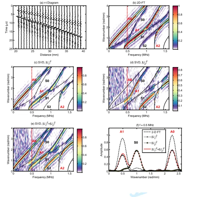
thick bone-mimicking plate with our array transducer. As shown in Fig. 1a, the 24 channel synthetic 9
wideband signals excited by first emitter are plotted in a time-distance (r-t) diagram. Signals corresponding 10
to six fundamental wide k-band (0<k<4 rad/mm) Lamb modes A0, S0, A1, S1, A2 and S2 were synthesized 11
according to [26], with peak-to-peak amplitudes of 1, 0.3, 1, 0.3, 1, and 0.3, respectively. A Gaussian noise 12
was added into each channel of the signal array with a fixed SNR of 15dB. The 2-D FT result of the received 13
signal after the first emission is presented in Fig. 1b, where the low-amplitude modes (S0, S1 and S2) are 14
too low to be identified. Fig. 1c depicts the first partial Norm function obtained using only the first singular 15
vector 𝑈1 (corresponding to the highest singular value) at each frequency. Fig. 1d shows the second partial
16
Norm function corresponding to the second singular vectors 𝑈2. Fig. 1e shows the Norm function calculated 17 2 3 4 5 6 7 8 9 10 11 12 13 14 15 16 17 18 19 20 21 22 23 24 25 26 27 28 29 30 31 32 33 34 35 36 37 38 39 40 41 42 43 44 45 46 47 48 49 50 51 52 53 54 55 56 57 58 59
For Review Only
according to Eq. (3) by summing these two partial functions, i.e., |𝑈1|2+ |𝑈2|2. Fig. 1f compares the
1
partial Norm functions with the wavenumber spectrum obtained using 2-D FT method at a fixed frequency 2
of 0.5 MHz. This particular frequency is indicated by red dot vertical lines in Figs. 1(b-e). The |𝑈1|2 and
3
|𝑈2|2 are shown with symbols (△ and ◇), respectively. The Norm function reconstructed by summing
4
amplitude-squares of two first singular vectors, i.e., |𝑈1|2+ |𝑈2|2 , is shown in red solid line. The
5
normalized 2-D FT results of the first emission is shown with black dash line. Compared with the 2D-FT 6
method, the SVD-based method enables to detect the dispersion trajectories for the weak modes. For 7
example, the low-amplitude S0 mode obtained by 2D-FT (see Fig. 1b) is significantly enhanced by using 8
SVD-based method (see Figs. 1e), which can also be confirmed in Fig. 1f by comparing the dash and solid 9
lines obtained by using two different methods. 10 2 3 4 5 6 7 8 9 10 11 12 13 14 15 16 17 18 19 20 21 22 23 24 25 26 27 28 29 30 31 32 33 34 35 36 37 38 39 40 41 42 43 44 45 46 47 48 49 50 51 52 53 54 55 56 57 58 59 60
For Review Only
1
Fig. 1. The synthetic signals, (a) distance-time (r-t) diagram, (b) dispersion energy in (𝑘, 𝑓) space using 2-D FT method,
2
(c) first partial Norm function obtained with the first singular vectors |𝑈1|2 corresponding to the highest singular values
3
for all frequencies, (d) second partial Norm function of second singular vectors |𝑈2|2 for all frequencies, (e) Norm function
4
obtained by summing two first singular vectors |𝑈1|2 and |𝑈2|2, i.e., |𝑈1|2+ |𝑈2|2, for all frequencies, (f) comparison of
5
the wavenumber functions obtained using SVD-based method and 2-D FT method at 0.5 MHz. Please note that the |·|2 is
6
the amplitude-square of each element of the matrix. 7 20 25 30 35 40 0 5 10 15 20 25 Distance (mm) T im e ( s) (a) r-t Diagram (b) 2D-FT Frequency (MHz) W a ve n u m b e r (r a d /m m ) A0 S0 A1 S1 S2 A2 0 0.5 1 1.5 0 1 2 3 4 0.2 0.4 0.6 0.8 1 (c) SVD, |U1|2 Frequency (MHz) W a ve n u m b e r (r a d /m m ) A0 S0 A1 S1 S2 A2 0 0.5 1 1.5 0 1 2 3 4 0.2 0.4 0.6 0.8 (d) SVD, |U2|2 Frequency (MHz) W a ve n u m b e r (r a d /m m ) A0 S0 A1 S1 S2 A2 0 0.5 1 1.5 0 1 2 3 4 0.1 0.2 0.3 0.4 0.5 0.6 0.7 0.8 (e) SVD, |U 1| 2+|U 2| 2 Frequency (MHz) W a ve n u m b e r (r a d /m m ) A0 S0 A1 S1 S2 A2 0 0.5 1 1.5 0 1 2 3 4 0.2 0.4 0.6 0.8 0 0.5 1 1.5 2 2.5 0 0.2 0.4 0.6 0.8 1 Wavenumber (rad/mm) A m p li tu d e (f) f = 0.5 MHz A1 S0 A0 2-D FT |U 1| 2 |U 2| 2 |U 1| 2+|U 2| 2 2 3 4 5 6 7 8 9 10 11 12 13 14 15 16 17 18 19 20 21 22 23 24 25 26 27 28 29 30 31 32 33 34 35 36 37 38 39 40 41 42 43 44 45 46 47 48 49 50 51 52 53 54 55 56 57 58 59
For Review Only
(2). Regularization parameter 𝜇 and hyperparameter 𝜎
1
Optimization of the factor 𝜇 and hyperparameter 𝜎 ensures the fidelity and the stability of the 2
regularization penalty. Fig. 2 shows the ‖𝑊(𝑘, 𝐸, 𝑓𝑝)‖𝐹2 curves of the multimodal signals in Fig. 1 versus 3
common logarithm 𝑙𝑜𝑔10(𝜇) for the frequency fixed at 1 MHz. It can be found that the ‖𝑊(𝑘, 𝐸, 𝑓𝑝)‖𝐹2 4
curve based on the LS-SVD method shows a constant norm without sparse property, whereas the 5
‖𝑊(𝑘, 𝐸, 𝑓𝑝)‖𝐹2 results of S-SVD present a left-right-flipped-Z-shape trend with two turning points. The 6
first turning points of S-SVD (𝑙1-norm) and S-SVD (Cauchy norm) on the ‖𝑊(𝑘, 𝐸, 𝑓𝑝)‖𝐹2 curves occur
7
around 𝜇 = 101.5 and 10‐1.5, respectively, which can achieve the sparse results. The second turning points
8
of S-SVD (𝑙1-norm) and S-SVD (Cauchy norm) on the ‖𝑊(𝑘, 𝐸, 𝑓𝑝)‖𝐹2 curves occur at 𝜇 = 106 and 10,
9
respectively, which actually indicates the change between high resolution and no sparsity. High reslution 10
results with different sparse degrees can be obtained in between of the two turning points. 11
12
Fig. 2. The ‖𝑊(𝑘, 𝐸, 𝑓𝑝)‖𝐹2 variation versus 𝑙𝑜𝑔10(𝜇) using different penalty functions, for the multimodal synthetic
13 signals at 1 MHz. 14 -10 -5 0 5 10 0 4 8 12 16 Sparse No Sparse High Resolution log 10() || W (k, E ,f p )| | 2 F LS-SVD l 1 Norm Cauchy Norm 1st Turning Points 2nd Turning Points 2 3 4 5 6 7 8 9 10 11 12 13 14 15 16 17 18 19 20 21 22 23 24 25 26 27 28 29 30 31 32 33 34 35 36 37 38 39 40 41 42 43 44 45 46 47 48 49 50 51 52 53 54 55 56 57 58 59 60
For Review Only
According to Eq. (10), if the value of hyperparameter 𝜎 is too large compared to that of |𝑊(𝑘, 𝐸, 𝑓𝑝)|, 1
the reweighting matrix 𝑄 will be only determined by the value of 𝜎. The value of 𝜎 should be much smaller 2
than the magnitude of |𝑊(𝑘, 𝐸, 𝑓𝑝)|. An heuristic value of 0.02 was adopted for 𝜎 in the present study. 3
Commonly, a relatively small value of regulation parameter 𝜇 leads to solutions with the best fit and 4
insignificant estimation error, while large 𝜇 can enhance the penalty effects with high-resolution sparsity 5
[15, 44, 45, 47]. However, due to the use of the inverse matrix 𝑈−1 in our model in Eq. (4), an opposite 6
relationship is observed between the sparsity and the regularization parameter. As shown in Fig. 2, a small 7
value of 𝜇 can guarantee the sparse convergence of the S-SVD method, while the use of a large 𝜇 value 8
actually is corresponding to no sparse results as similar as the LS-SVD method. Furthermore, 𝜇 = 0 cannot 9
achieve the correct reweighting either. Those statuses between the first and second turning points can be 10
used to tune the sparsity with different resolutions. 11
(3). LS-SVD and high-resolution sparse SVD results of the synthetic data
12
Figure 3 shows the Norm functions obtained by applying SVD, LS-SVD, and S-SVD (𝑙1-norm and
13
Cauchy norm) to the synthetic signals. Compared with the 2-D FT results (in Fig. 1), the low amplitude 14
modes (S0, S1 and S2) are successfully enhanced by the SVD-based processing in Fig. 3a. As shown in 15
Fig. 3b, there is no improvement of the wavenumber resolution using the LS-SVD method ( also see Fig. 16
4). Figs. 3(c-f) present the S-SVD results with different resolution, two group of different regularization 17
parameters, i.e., 𝜇 = 0.5, 1000 and 𝜇 = 0.01, 1, are used for S-SVD (𝑙1-norm) and S-SVD (Cauchy norm), 18
respectively. It can be observed that the small 𝜇 selected around the first turning point of Fig. 2 yields high-19
sparse estimates of the dispersion curves (Figs. 3c and 3e). Furthermore, choosing the suitable 𝜇 values, 20 2 3 4 5 6 7 8 9 10 11 12 13 14 15 16 17 18 19 20 21 22 23 24 25 26 27 28 29 30 31 32 33 34 35 36 37 38 39 40 41 42 43 44 45 46 47 48 49 50 51 52 53 54 55 56 57 58 59
For Review Only
the S-SVD method can converge to different sparse levels (Figs. 3d and 3f) with different resolutions (also 1
see Fig. 4). The convergence characteristics actually change with the frequencies, but Fig. 3 also confirmed 2
that 𝜇 is stable enough to achieve a similar sparse level at different frequencies. 3
4
Fig. 3. Norm functions obtained using SVD, LS-SVD, S-SVD (𝑙1-norm, and Cauchy norm) applied to the synthetic
5
signals corresponding to a 2 mm-thick bone-mimicking plate.
6 (a) SVD Frequency (MHz) W a ve n u m b e r (r a d /m m ) A0 S0 A1 S1 S2 A2 0 0.5 1 1.5 0 1 2 3 4 (b) LS-SVD, ( = 100) Frequency (MHz) W a ve n u m b e r (r a d /m m ) A0 S0 A1 S1 S2 A2 0 0.5 1 1.5 0 1 2 3 4 (c) S-SVD (l 1), (,) = (0.5, 0.02) Frequency (MHz) W a ve n u m b e r (r a d /m m ) A0 S0 A1 S1 S2 A2 0 0.5 1 1.5 0 1 2 3 4 (d) S-SVD (l 1), (,) = (1000, 0.02) Frequency (MHz) W a ve n u m b e r (r a d /m m ) A0 S0 A1 S1 S2 A2 0 0.5 1 1.5 0 1 2 3 4 (e) S-SVD (Cauchy), (,) = (0.01, 0.02) Frequency (MHz) W a ve n u m b e r (r a d /m m ) A0 S0 A1 S1 S2 A2 0 0.5 1 1.5 0 1 2 3 4 (f) S-SVD (Cauchy), (,) = (1, 0.02) Frequency (MHz) W a ve n u m b e r (r a d /m m ) A0 S0 A1 S1 S2 A2 0 0.5 1 1.5 0 1 2 3 4 2 3 4 5 6 7 8 9 10 11 12 13 14 15 16 17 18 19 20 21 22 23 24 25 26 27 28 29 30 31 32 33 34 35 36 37 38 39 40 41 42 43 44 45 46 47 48 49 50 51 52 53 54 55 56 57 58 59 60
For Review Only
1
Fig. 4. Comparison of wavenumber resolution at 1 MHz of the synthetic signals corresponding to a 2 mm-thick
bone-2
mimicking plate.
3
Figure 4 compares the Norm function obtained at 1 MHz (indicated as red dot lines in Fig. 3) using 4
different methods and different parameters. The SVD and LS-SVD provide comparable results with the 5
same resolution as that of the 2-D FT. In this study, the wavenumber resolution corresponding to the probe 6
employed can be computed by 2 ∗ 2𝜋 (24 ∗ 0.8)⁄ = 0.65 rad/mm, where the 24 and 0.8 mm are number 7
of the elements and pitch size, respectively. For example, the main lobe width of S2 mode, extracted by the 8
SVD and LS-SVD method, is equal to 0.65 rad/mm locating between 0.54 and 1.19 rad/mm in Fig. 4. An 9
improved resolution is reached using the S-SVD method. For instance, the main lobe of the S2 mode 10
extracted from the amplitude curves of S-SVD (Cauchy, 𝜇 = 0.01) has a width of 0.11 rad/mm, i.e., 6 11
times improvement compared to the classical 2-D FT resolution, approximately. As shown in Fig. 2, such 12
a 𝜇 value is adopted according the first turning point. It also illustrates that using the S-SVD method, only 13
3 sharp peaks are observed and the mode energy leakage is completely suppressed. However, with such a 14
wavenumber resolution obtained by S-SVD, it is still not high enough to resolve those severely overlapped 15
modes, such as A1 and S1 modes in range of 0.7 to 1 rad/mm. 16 0 0.5 1 1.5 2 2.5 3 3.5 4 0 0.2 0.4 0.6 0.8 1 Wavenumber (rad/mm) A m p lit u d e Resolution Comparison SVD LS-SVD ( = 100) S-SVD (l1, = 0.5) S-SVD (l 1, = 1000) S-SVD (Cauchy, = 0.01) S-SVD (Cauchy, = 1) 2 3 4 5 6 7 8 9 10 11 12 13 14 15 16 17 18 19 20 21 22 23 24 25 26 27 28 29 30 31 32 33 34 35 36 37 38 39 40 41 42 43 44 45 46 47 48 49 50 51 52 53 54 55 56 57 58 59
For Review Only
B. Phantom experiment
1
Figure 5 displays the SVD and S-SVD results of the experiment signal measured in the 4 mm-thick 2
Sawbone plates. The results are also presented in (𝑘, 𝑓) domain with the wavenumber dispersion curves. 3
Similarly to the results of synthetic signals, the S-SVD method can improve the extraction of the dispersion 4
curves with sparse energy focusing and noise filtering. 5
The main lobes of the S0 and A1 mode illustrated from the amplitude curves of the S-SVD (Cauchy 6
norm) with (𝜇, 𝜎) = (0.0015, 0.02) and S-SVD (𝑙1-norm) with (𝜇, 𝜎) = (10, 0.02) are in widths of 0.28
7
rad/mm and 0.18 rad/mm, respectively. In particular, the Norm function extracted at 1 MHz in the range of 8
1 to 2 rad/mm shows that the sparse SVD (Cauchy norm) enables to separate two wavenumber peaks, and 9
the sparse SVD (𝑙1-norm) finds three wavenumber peaks, when the SVD finds a single large peak (see Fig.
10
5d). Actually, in this wavenumber range, the plate model predicts the presence of two pairs of close modes 11
A2, S2 and A3, S3, respectively. The wavenumber resolution enhancement achieved with S-SVD, in 12
contrast to SVD, allows separation of the two pairs of close modes. The finest resolution of S-SVD (𝑙1
-13
norm) even enables recovering A2 and S2 from the data, the third peak corresponding to the overlapping 14
A3 and S3 modes. Similar case can also be observed in the range of 2 to 4 rad/mm, where the S-SVD (𝑙1
-15
norm and Cauchy norm) method is able to retrieve the relatively weak peaks of A1, S0 and S1 modes which 16
are highly overlapped together. 17 2 3 4 5 6 7 8 9 10 11 12 13 14 15 16 17 18 19 20 21 22 23 24 25 26 27 28 29 30 31 32 33 34 35 36 37 38 39 40 41 42 43 44 45 46 47 48 49 50 51 52 53 54 55 56 57 58 59 60
For Review Only
1
Fig. 5. Multimode dispersion curves measured in a 4 mm-thick bone-mimicking plate, SVD and S-SVD (𝑙1-norm and
2
Cauchy norm) results, comparison of wavenumber resolution at 1 MHz. 3
C. Ex-vivo experiments
4
Results presented in Fig. 6 refer to the signals measured in a 2.5 mm-thick human radius ex vivo. Due 5
to low SNR, the Norm function illustrated in the Fig. 6a is corrupted by the noise. Meanwhile the aperture 6
limit in clinical measurement still induces strong mode aliasing, which is challenging for mode 7
identification. As shown in Figs. 6b and 6c, in agreement with the simulation and phantom studies, the S-8
SVD method can filter most of the noise and yields energy concentrated trajectories. Because at 1 MHz, 9
some modes, like S0, S1 and A1 are poorly excited, the amplitude curves at 0.5 MHz are plotted in Fig. 6d, 10
which also confirms the high wavenumber resolution of the S-SVD method. The main lobes of the A0 11 (a) SVD Frequency (MHz) W a ve n u m b e r (r a d /m m ) A0 S0 A1 S1 A2 S2 A3 S3 A4 S4 S5 0 0.5 1 1.5 0 1 2 3 4 (b) S-SVD(l1), (,) = (10, 0.02) Frequency (MHz) W a ve n u m b e r (r a d /m m ) A0 S0 A1 S1 A2 S2 A3 S3 A4 S4 S5 0 0.5 1 1.5 0 1 2 3 4 (c) S-SVD(Cauchy), (,) = (0.0015, 0.02) Frequency (MHz) W a ve n u m b e r (r a d /m m ) A0 S0 A1 S1 A2 S2 A3 S3 A4 S4 S5 0 0.5 1 1.5 0 1 2 3 4 0 1 2 3 4 0 0.5 1 1.5 Wavenumber (rad/mm) A m p lit u d e (d) Resolution Comparison SVD S-SVD(l1) S-SVD(Cauchy) 2 3 4 5 6 7 8 9 10 11 12 13 14 15 16 17 18 19 20 21 22 23 24 25 26 27 28 29 30 31 32 33 34 35 36 37 38 39 40 41 42 43 44 45 46 47 48 49 50 51 52 53 54 55 56 57 58 59
For Review Only
mode illustrated from the amplitude curves of the S-SVD (𝑙1-norm) with (𝜇, 𝜎) = (500, 0.02) and S-SVD
1
(Cauchy norm) with (𝜇, 𝜎) = (0.2, 0.02) are in widths of 0.22 rad/mm and 0.20 rad/mm, respectively. 2
3
Fig. 6. Multimode dispersion curves measured in a 2.5 mm-thick human radius (ex vivo), SVD and S-SVD (𝑙1-norm,
4
and Cauchy norm) results, comparison of wavenumber resolution at 0.5 MHz.
5
V. DISCUSSION 6
The main motivation of this study comes from the limitation encountered in extraction of the 7
dispersion curves when the time signals are recorded using receiving array of limited aperture with a 8
measurable length of several centimeters where only tense of transducer elements can actually be arranged. 9
The limitation is due to accessibility of clinical sites such as forearm. Currently, a SVD-based signal 10 (a) SVD Frequency (MHz) W a ve n u m b e r (r a d /m m ) A0 S0 A1 S1 S2 A2 0 0.5 1 1.5 0 1 2 3 4 (b) S-SVD(l1), (,) = (500, 0.02) Frequency (MHz) W a ve n u m b e r (r a d /m m ) A0 S0 A1 S1 S2 A2 0 0.5 1 1.5 0 1 2 3 4 (c) S-SVD(Cauchy), (,) = (0.2, 0.02) Frequency (MHz) W a ve n u m b e r (r a d /m m ) A0 S0 A1 S1 S2 A2 0 0.5 1 1.5 0 1 2 3 4 0 1 2 3 4 0 0.5 1 1.5 Wavenumber (rad/mm) A m p lit u d e (d) Resolution Comparison SVD S-SVD(l 1) S-SVD(Cauchy) 2 3 4 5 6 7 8 9 10 11 12 13 14 15 16 17 18 19 20 21 22 23 24 25 26 27 28 29 30 31 32 33 34 35 36 37 38 39 40 41 42 43 44 45 46 47 48 49 50 51 52 53 54 55 56 57 58 59 60
For Review Only
processing approach allows efficient noise filtering and weak modes amplitude enhancement. However, 1
the relatively poor spatial sampling results in poor resolution on the wavenumber k-axis, which still 2
prevents a clear identification of the dispersion curves of overlapping modes. The sparse strategy continues 3
to attract considerable attention with capability of resolution improvement beyond the classical resolution 4
limit. In this paper, a S-SVD method for sparse characterization of the dispersion curves is proposed to 5
overcome the limited wavenumber resolution of ultrasonic guided waves measurement. The method is 6
proposed, assuming that the additional noise, which is weakly correlated to the singular vectors of the SVD 7
decomposition, can be optimally removed to promote a sparse result. 8
In agreement with previous studies [15, 40, 44, 45], our results also illustrate that the choice of the 9
penalty term is important for the sparse optimization. The use of the 𝑙2-norm penalty in our cost function
10
basically leads to the least-squares solution, without obvious improvement of the wavenumber resolution. 11
Furthermore, it seems that the proposed LS-SVD method cannot effectively remove the additive noise 12
either. In contrast, the use of 𝑙1-norm and Cauchy norm can enhance the extraction of the dispersion curves
13
with a high wavenumber resolution, i.e., sparse characteristics [15, 44, 45]. As illustrated in the synthetic 14
and experimental results, both 𝑙1-norm and Cauchy penalty terms can provide good results with significant
15
resolution enhancement, so that it is difficult to directly conclude which of them can provide the finest 16
Norm function with the best wavenumber resolution. Certainly, other penalty terms are also worth to be
17
investigated, for instance the 𝑙𝑝-norm or even some polynomial terms (the sum of different norms). The 18
trade-off could be that the complicated design of the cost function will also raise other challenges, such as 19
the optimization of the regularization factors and the convergence criteria. 20 2 3 4 5 6 7 8 9 10 11 12 13 14 15 16 17 18 19 20 21 22 23 24 25 26 27 28 29 30 31 32 33 34 35 36 37 38 39 40 41 42 43 44 45 46 47 48 49 50 51 52 53 54 55 56 57 58 59
For Review Only
Regularization schemes are commonly accepted to solve ill-posed problems. The performance of S-1
SVD method highly relies on the choice of a suitable regularization parameter. Unsuitable regularization 2
will either enforce the over-sparse effectiveness to the all-zero solution or provide an insufficient sparse 3
solution without enough enhancement. We used an heuristic method to optimize the regularization 4
parameter. As shown in Fig. 2, when the regularization parameter increases, the norm ‖𝑊̃ (𝑘, 𝐸, 𝑓𝑝)‖
𝐹 2
5
convergence curves present two turning points with the left-right-flipped-Z-shape trends. The first and 6
second turning points of the ‖𝑊̃ (𝑘, 𝐸, 𝑓𝑝)‖𝐹2 curve are on the boundaries of the sparsity, high-resolution 7
and no-sparsity, respectively. The results suggest that the first turning point can be chosen as the suitable 8
value of the regularization parameter with sparsity optimization. Furthermore, the values of the 9
regularization parameter between the two turning points enable to tune the sparse level with different 10
resolutions. A second hyperparameter 𝜎 is imposed on the penalty function. It can be understood as a small 11
additive perturbation that represents the default power in absence of hyperbolic events [32]. A 1-D search 12
based on Brent parabolic interpolation could be used to optimize 𝜎 [43, 48]. However, it should be noted 13
that the convergence characteristics also vary with frequencies. Strictly speaking, the regularization 14
parameter and hyperparameter must be optimized at each frequency. In our study, we find that they are 15
stable enough to allow us to choose identical values for different frequencies. Furthermore, there is also a 16
trade-off between the sparsity/resolution and capability of mode retrieve, since the very high resolution also 17
enhances the over-sparse effectiveness with drawback of removing some of the useful information. To 18
maximize the dispersion information, a suitable sparse level should be chosen with balance between the 19
misfit and resolution, allowing to remaining the weak modes together with sufficient separation of the 20
overlap dispersion curves. 21 2 3 4 5 6 7 8 9 10 11 12 13 14 15 16 17 18 19 20 21 22 23 24 25 26 27 28 29 30 31 32 33 34 35 36 37 38 39 40 41 42 43 44 45 46 47 48 49 50 51 52 53 54 55 56 57 58 59 60
For Review Only
Other signal processing methods, such as the spectrum estimation and high-resolution Radon method 1
[15, 44, 45] can also be considered to achieve a high-resolution wavenumber distribution. However, to the 2
best authors’ knowledge, currently, most of the proposed methods have been designed for single-emitter 3
multi-receiver processing. In contrast, our SVD-based approach takes advantage of both the multichannel 4
transmission and reception. Specifically, the proposed S-SVD method combines the advantages of the 5
SVD-based enhancement of low-amplitude modes and also of the sparse penalty scheme to filter the noise 6
with high wavenumber resolution. Such a method may be more robust for detecting those weak modes 7
severely corrupted by noise, especially when measuring highly damping materials, such as bone. 8
The S-SVD method developed in the study involves matrix inversion in the SVD iteration with a 9
relatively expensive computation. However, in general, 10 to 20 times iterations are sufficient to converge 10
to the sparse solution, which suggests that the S-SVD method is capable for the real-time multi-emitter and 11
multi-receiver data processing. 12
VI. CONCLUSION 13
This original S-SVD approach discussed in this study combines the SVD-based SNR improvement 14
and the advantage of sparse regularization strategy to successfully achieve high resolution extraction of the 15
dispersion curves of ultrasonic guided waves. The analysis of the synthetic signals and experimental data 16
illustrates that the S-SVD method may provide significant advantages when trying to retrieve the 17
characteristics of the waveguide using model-based inverse procedures for three reasons: 18
i) The sparse strategy can overcome the practical problem of the finite aperture caused by the 19
limit size and small number of elements of the probe. The S-SVD method allows retrieving 20 2 3 4 5 6 7 8 9 10 11 12 13 14 15 16 17 18 19 20 21 22 23 24 25 26 27 28 29 30 31 32 33 34 35 36 37 38 39 40 41 42 43 44 45 46 47 48 49 50 51 52 53 54 55 56 57 58 59
For Review Only
the dispersion curves with high wavenumber resolution, so that some severely overlapping 1
guided modes can be separated; 2
ii) The merits of the SVD-based method and the high resolution optimization are preserved, 3
which allows extraction of some weak modes severely corrupted by noise; 4
iii) The robust convergence characteristics of the regularization parameters allow the convenient 5
implementation of the S-SVD method. Furthermore, the left-right-flipped-Z-shape trend of the 6
sparse Norm function provides a flexible way for tuning the sparsity of the dispersion 7
trajectories for different applications. 8
The existence of surrounding soft tissues is expected to affect the SNR and signal coherence. Future 9
work will focus on adapting the S-SVD method on processing the in vivo guided waves data. 10
VII. ACKNOWLEDGMENT 11
The authors also acknowledge Dr. Maryline Talmant and Dr. Didier Cassereau in Laboratoire 12
d’Imagerie Biomédicale (LIB) and Dr. Qi Zhou from the Department of Mathematics, Nanjing University, 13
for their constructive comments and excellent advices to improve the paper. This work was supported by 14
the National Natural Science Foundation of China (11304043, 11327405, 11525416), the NSFC-CNRS-15
PICS (11511130133), the CNRS PICS programme n°07032 and the Fondation pour la Recherche Medicale 16
through project number FRM DBS201311228444. 17
18
References:
19[1] C. H. Chapman, "A new method for computing synthetic seismograms," Geophysical Journal International, vol. 54, pp. 20 481-518, 1978. 21 2 3 4 5 6 7 8 9 10 11 12 13 14 15 16 17 18 19 20 21 22 23 24 25 26 27 28 29 30 31 32 33 34 35 36 37 38 39 40 41 42 43 44 45 46 47 48 49 50 51 52 53 54 55 56 57 58 59 60
For Review Only
[2] G. A. McMechan and M. J. Yedlin, "Analysis of dispersive waves by wave field transformation," Geophysics, vol. 46, pp. 1
869-874, 1981. 2
[3] P. Gabriels, R. Snieder and G. Nolet, "In situ measurements of shear-wave velocity in sediments with higher-mode Rayleigh 3
waves," Geophysical prospecting, vol. 35, pp. 187-196, 1987. 4
[4] C. B. Park, R. D. Miller and J. Xia, "Multichannel analysis of surface waves," Geophysics, vol. 64, pp. 800-808, 1999. 5
[5] G. D. Bensen, M. H. Ritzwoller, M. P. Barmin, A. L. Levshin, F. Lin, M. P. Moschetti, N. M. Shapiro, and Y. Yang, 6
"Processing seismic ambient noise data to obtain reliable broad-band surface wave dispersion measurements," Geophysical 7
Journal International, vol. 169, pp. 1239-1260, 2007.
8
[6] Y. Luo, J. Xia, R. D. Miller, Y. Xu, J. Liu, and Q. Liu, "Rayleigh-wave dispersive energy imaging using a high-resolution 9
linear Radon transform," Pure and Applied Geophysics, vol. 165, pp. 903-922, 2008. 10
[7] A. Papandreou-Suppappola, R. L. Murray, B. G. Iem, and G. F. Boudreaux-Bartels, "Group delay shift covariant quadratic 11
time-frequency representations," IEEE Transactions on Signal Processing, vol. 49, pp. 2549-2564, 2001. 12
[8] G. Le Touze, B. Nicolas, J. I. Mars, and J. L. Lacoume, "Matched representations and filters for guided waves," IEEE 13
Transactions on Signal Processing, vol. 57, pp. 1783-1795, 2009.
14
[9] J. Bonnel, G. E. G. Le Touz E, B. Nicolas, and J. Mars, IEEE Signal Processing Magazine, vol. 30, pp. 120-129, 2013. 15
[10] D. Alleyne and P. Cawley, "A two-dimensional Fourier transform method for the measurement of propagating multimode 16
signals," Journal of the Acoustical Society of America, vol. 89, pp. 1159-1168, 1991. 17
[11] W. H. Prosser, M. D. Seale and B. T. Smith, "Time-frequency analysis of the dispersion of Lamb modes," Journal of the 18
Acoustic Society of America, vol. 105, pp. 2669-2676, 1999.
19
[12] P. Wilcox, M. Lowe and P. Cawley, "The effect of dispersion on long-range inspection using ultrasonic guided waves," 20
NDT&E International, vol. 34, pp. 1-9, 2001.
21
[13] S. Fateri, N. V. Boulgouris, A. Wilkinson, W. Balachandran, and T. Gan, IEEE Transactions on Ultrasonics, Ferroelectrics, 22
and Frequency Control, vol. 61, pp. 1515-1524, 2014.
23
[14] K. Xu, D. Ta and W. Wang, "Multiridge-based analysis for separating individual modes from multimodal guided wave 24
signals in long bones," IEEE Transactions on Ultrasonics, Ferroelectrics and Frequency Control, vol. 57, pp. 2480-2490, 2010. 25
[15] T. N. Tran, K. T. Nguyen, M. D. Sacchi, and L. H. Le, "Imaging ultrasonic dispersive guided wave energy in long bones 26
using linear Radon transform," Ultrasound in Medicine and Biology, vol. 40, pp. 2715-2727, 2014-11-01 2014. 27
[16] J. Foiret, J. G. Minonzio, C. Chappard, M. Talmant, and P. Laugier, "Combined estimation of thickness and velocities using 28
ultrasound guided waves: a pioneering study on in vitro cortical bone samples," IEEE Transactions on Ultrasonics, 29
Ferroelectrics and Frequency Control, vol. 61, pp. 1478-1488, 2014.
30
[17] M. Bernal, I. Nenadic, M. W. Urban, and J. F. Greenleaf, "Material property estimation for tubes and arteries using 31
ultrasound radiation force and analysis of propagating modes," Journal of the Acoustical Society of America, vol. 129, pp. 1344-32
1354, 2011. 33
[18] J. Xia, Y. Xu and R. D. Miller, "Generating an image of dispersive energy by frequency decomposition and slant stacking," 34
Pure and Applied Geophysics, vol. 164, pp. 941-956, 2007.
35
[19] J. G. Minonzio, M. Talmant and P. Laugier, "Guided wave phase velocity measurement using emitter and multi-36
receiver arrays in the axial transmission configuration," Journal of the Acoustical Society of America, vol. 127, pp. 2913-2919, 37
2010. 38
[20] L. Wang, Y. Xu, J. Xia, and Y. Luo, "Effect of near-surface topography on high-frequency Rayleigh-wave propagation," 39
Journal of Applied Geophysics, vol. 116, pp. 93-103, 2015.
40
[21] L. Cohen, "Time-frequency distributions-a review," Proceedings of the IEEE, vol. 77, pp. 941-981, 1989. 41 2 3 4 5 6 7 8 9 10 11 12 13 14 15 16 17 18 19 20 21 22 23 24 25 26 27 28 29 30 31 32 33 34 35 36 37 38 39 40 41 42 43 44 45 46 47 48 49 50 51 52 53 54 55 56 57 58 59
For Review Only
[22] L. De Marchi, A. Marzani, S. Caporale, and N. Speciale, "Ultrasonic guided-waves characterization with warped frequency 1
transforms," IEEE Transactions on Ultrasonics, Ferroelectrics and Frequency Control, vol. 56, pp. 2232-2240, 2009. 2
[23] M. Zhao, L. Zeng, J. Lin, and W. Wu, "Mode identification and extraction of broadband ultrasonic guided waves," 3
Measurement Science and Technology, vol. 25, p. 115005, 2014.
4
[24] Y. Yang, Z. K. Peng, W. M. Zhang, G. Meng, and Z. Q. Lang, "Dispersion analysis for broadband guided wave using 5
generalized warblet transform," Journal of Sound and Vibration, vol. 367, pp. 22-36, 2016. 6
[25] J. Hong, K. H. Sun and Y. Y. Kim, "Dispersion-based short-time Fourier transform applied to dispersive wave analysis," 7
Journal of the Acoustical Society of America, vol. 117, pp. 2949-2960, 2005.
8
[26] K. Xu, D. Ta, P. Moilanen, and W. Wang, "Mode separation of Lamb waves based on dispersion compensation method," 9
Journal of the Acoustical Society of America, vol. 131, pp. 2714-2722, 2012.
10
[27] R. Sicard, J. Goyette and D. Zellouf, "A numerical dispersion compensation technique for time recompression of Lamb 11
wave signals," Ultrasonics, vol. 40, pp. 727-732, 2002. 12
[28] P. D. Wilcox, "A rapid signal processing technique to remove the effect of dispersion from guided wave signals," IEEE 13
Transactions on Ultrasonics, Ferroelectrics and Frequency Control, vol. 50, pp. 419-427, 2003.
14
[29] P. Moilanen, "Ultrasonic guided waves in bone," IEEE Transactions on Ultrasonics, Ferroelectrics and Frequency Control, 15
vol. 55, pp. 1277-1286, 2008. 16
[30] D. Trad, T. Ulrych and M. Sacchi, "Latest views of the sparse Radon transform," Geophysics, vol. 68, pp. 386-399, 2003. 17
[31] J. R. Thorson and J. F. Claerbout, "Velocity-stack and slant-stack stochastic inversion," Geophysics, vol. 50, pp. 2727-2741, 18
1985. 19
[32] M. D. Sacchi and T. J. Ulrych, "High-resolution velocity gathers and offset space reconstruction," Geophysics, vol. 60, p. 20
1169, 1995. 21
[33] R. O. Schmidt, "Multiple emitter location and signal parameter estimation," IEEE Transactions on Antennas and 22
Propagation, vol. 34, pp. 276-280, 1986.
23
[34] J. G. Minonzio, J. Foiret, M. Talmant, and P. Laugier, "Impact of attenuation on guided mode wavenumber measurement 24
in axial transmission on bone mimicking plates," Journal of the Acoustical Society of America, vol. 130, pp. 3574-3582, 2011. 25
[35] M. Talmant, J. Foiret and J. G. Minonzio, "Guided waves in cortical bone," in Bone quantitative ultrasound Dordrecht, 26
Heidelberg, London, New York: Springer, 2011, pp. 147-179. 27
[36] J. G. Minonzio, J. Foiret, P. Moilanen, J. Pirhonen, Z. Zhao, M. Talmant, J. Timonen, and P. Laugier, "A free plate model 28
can predict guided modes propagating in tubular bone-mimicking phantoms," Journal of the Acoustical Society of America, vol. 29
137, pp. EL98-EL104, 2015. 30
[37] F. Lefebvre, Y. Deblock, P. Campistron, D. Ahite, and J. J. Fabre, "Development of a new ultrasonic technique for bone 31
and biomaterials in vitro characterization," Journal of Biomedical Materials Research, vol. 63, pp. 441-446, 2002. 32
[38] P. Moilanen, Z. Zhao, P. Karppinen, T. Karppinen, V. Kilappa, J. Pirhonen, R. Myllylä, E. Hæggström, and J. Timonen, 33
"Photo-acoustic Excitation and Optical Detection of Fundamental Flexural Guided Wave in Coated Bone Phantoms," Ultrasound 34
in Medicine & Biology, vol. 40, pp. 521-531, 2014.
35
[39] I. A. Viktorov, Rayleigh and Lamb waves: physical theory and applications: Plenum press New York, 1967. 36
[40] J. B. Harley and J. M. F. Moura, "Sparse recovery of the multimodal and dispersive characteristics of Lamb waves," Journal 37
of the Acoustical Society of America, vol. 133, p. 2732, 2013.
38
[41] C. B. Park, "Imaging dispersion curves of surface waves on multi-channel record," SEG Technical Program Expanded 39
Abstracts, vol. 17, p. 1377, 1999.
40
[42] K. Xu, J. G. Minonzio, D. Ta, B. Hu, W. Wang, and P. Laugier, "Sparse inversion SVD method for dispersion extraction 41 2 3 4 5 6 7 8 9 10 11 12 13 14 15 16 17 18 19 20 21 22 23 24 25 26 27 28 29 30 31 32 33 34 35 36 37 38 39 40 41 42 43 44 45 46 47 48 49 50 51 52 53 54 55 56 57 58 59 60
For Review Only
of ultrasonic guided waves in cortical bone," in 2015 6th European Symposium on Ultrasonic Characterization of Bone (ESUCB), 1
2015, pp. 1-3. 2
[43] M. D. Sacchi, "Reweighting strategies in seismic deconvolution," Geophysical Journal International, vol. 129, pp. 651-3
656, 1997. 4
[44] T. N. Tran, L. H. Le and M. D. Sacchi, "High-Resolution Imaging of Dispersive Ultrasonic Guided Waves in Human Long 5
Bones Using Regularized Radon Transforms," in 5th International Conference on Biomedical Engineering in Vietnam, 2015, 6
pp. 28-31. 7
[45] T. N. Tran, L. H. Le, M. D. Sacchi, V. Nguyen, and E. H. Lou, "Multichannel filtering and reconstruction of ultrasonic 8
guided wave fields using time intercept-slowness transform," Journal of the Acoustical Society of America, vol. 136, pp. 248-9
259, 2014. 10
[46] J. F. Claerbout, "Earth sounding analysis: Processing versus inversion," Blackwell Scientific Publications, Inc., 1992. 11
[47] P. C. Hansen and D. P. O'Leary, "The use of the L-curve in the regularization of discrete ill-posed problems," SIAM Journal 12
on Scientific Computing, vol. 14, pp. 1487-1503, 1993.
13
[48] W. H. Press, Numerical recipes 3rd edition: The art of scientific computing: Cambridge university press, 2007. 14 15 2 3 4 5 6 7 8 9 10 11 12 13 14 15 16 17 18 19 20 21 22 23 24 25 26 27 28 29 30 31 32 33 34 35 36 37 38 39 40 41 42 43 44 45 46 47 48 49 50 51 52 53 54 55 56 57 58 59