Computerized schedule construction for an airbus transportation system

'COMPUTERIZED SCHEDULE

CONSTRUCTION FOR AN AIRLINE

TRANSPORTATION SYSTEM

R.

W. Simpson

ARCHIVES

MASSACHUSETTS INSTITUTE OF TECHNOLOGY

FLIGHT TRANSPORTATION LABORATORY

Technical Report FT-66-3

December 1966

Computerized Schedule Construction for an Airbus

Transportation System

R. W. Simpson

This work was performed under Contract C-136-66 for

the Office of High Speed Ground Transport, Department of

Computerized Schedule Construction for an

Airbus Transportation System

R. W. Simpson

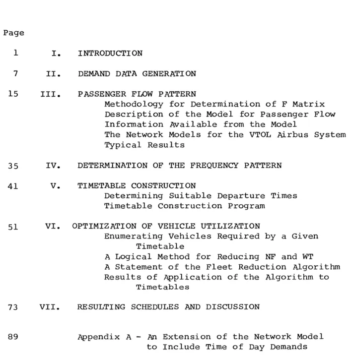
TABLE OF CONTENTS

Page

1 I. INTRODUCTION

7 II. DEMAND DATA GENERATION

15 III. PASSENGER FLOW PATTERN

Methodology for Determination of F Matrix Description of the Model for Passenger Flow Information Available from the Model

The Network Models for the VTOL Airbus System Typical Results

35 IV. DETERMINATION OF THE FREQUENCY PATTERN

41 V. TIMETABLE CONSTRUCTION

Determining Suitable Departure Times Timetable Construction Program

51 VI. OPTIMIZATION OF VEHICLE UTILIZATION

Enumerating Vehicles Required by a Given Timetable

A Logical Method for Reducing NF and WT

A Statement of the Fleet Reduction Algorithm Results of Application of the Algorithm to

Timetables

73 VII. RESULTING SCHEDULES AND DISCUSSION

89 Appendix A - An Extension of the Network Model

to Include Time of Day Demands

I. INTRODUCTION

As part of a continuing study of the application of

V/STOL aircraft to the transportation problems of the

Northeast Corridor, the U.S. Department of Commerce has

requested that detailed data be developed on schedules,

travel times, and fares which might be expected for a

V/STOL system operating in the year 1980. This section

deals with the computer methods used to construct such

schedules.

A schedule (or more properly a schedule plan) is a

complete description of a transportation system. It

de-tails the services to be offered in the dimensions

of time and geography, gives the routings followed by

vehicles, and indicates the loadings to be placed upon

terminals. A complete statistical summary of the

opera-tion of the transportaopera-tion system can be obtained once

the schedule is completed. The number of vehicles and

crews, their daily utilization, the expected load factors,

the required number of loading gates, the average length

of vehicle hop, etc. are all implicitly determined by the

schedule plan. Constructing and maintaining an efficient

schedule is the main problem of transportation system

managements. It is both their production plan and their

product to be marketed, and the economic success of the

plan is gauged by the management's ability to produce a

low cost production which will be saleable to the

travel-ling public.

The use of computers in scheduling is not widespread

at this time, and if they are used, it is generally for

data processing as distinct from decision making or problem

solving. The reasons for this are clear. There has not

been in the past, sufficient capability either in the

hard-ware, or the software to handle problems of the size and

complexity associated with even such relatively small

transportation systems.as the airline systems. This

situ-ation has been changing in the last few years, to the point

where we can now begin to handle fairly large scale

schedu-ling problems, introducing optimization at several points,

and constructing fairly quickly and easily full systen

schedules and their statistical summaries. Parametric

investigations of the effects of restricting fleet size,

terminal size, etc. can be quickly carried out. Various

strategies or policy decisions are similarly easily

inves-tigated.

-2-The construction of computer programs for the schedu-ling process immediately points out the need for detailed

accurate data concerning demand. This is now becoming

available to the airlines through their reservation

sys-tems and the management information syssys-tems evolving from

them. We need to know, for example, detailed information

on the number of people travelling from A to B throughout

the day, by day of week and month of year, with an accuracy

much greater than our present estimates. We would like to

know the demand elasticity, e.g. the change in the number

of people travelling as services are changed in time or

quality for every service pair in the system. The

charac-ter of the available data (as distinct from opinion) decharac-ter-

deter-mines the type of problem that operations research and the

computer will be able to successfully solve. Various large

scale econometric models are conceivable, if revenue and

cost data are available.

This section will describe the work which has been

carried out for a hypothetical Airbus short haul V/STOL

system in the Northeast Corridor. It is only a beginning

as valuable extensions are yet to come as more applications

-3-come into the open literature. The main presentation

will describe the computerized processes developed to

construct a schedule plan assuming certain demand and

operating data. An interesting extension showing the

application of network flow theory to a more detailed

representation of the schedule is then described in

Appendix A.

A map of the corridor showing the terminals selected

for the Airbus system is shown in Figure 1. Table

I shows

some typical distances, travel times, and projected fares

for

the 1980 Airbus.

-4-TABLE I

Typical Fares and Travel Times VTOL Airbus System

TRIP

Washington downtown

- Dulles

- Baltimore downtown - Philadelphia downtown - New York downtown

- Norfolk - Providence Distance (st. miles) 26 33 123 203 144 351 Time (minutes) 6 7 22 34 25 58 Fare (1966 dollars) 3.10 3.35 6.55 9.35 7.25 14.60 Boston downtown - Worcester - Providence - Hartford - Laguardia - Philadelphia downtown - New York downtown

From to From to 40 46 89 181 266 190 8 9 16 31 44 32 3.60 3.80 5.35 8.60 11.60 8.90

-5-0 30 60 miles _MANe FITe eWBA AM EWI ALL* REA* ISP-EQU LGA

STUDY AREA

NORTHEAST CORRIDOR TRANSPORTATION PROJECT UNITED STATES DEPARTMENT OF COMMERCE * MAJOR TERMINALS ' SMALL TERMINALS

VTOL AIRBUS TRANSPORTATION SYSTEM

FIG. I

-6-HARe,\

YRK. eLAN

II.

DEMAND DATA GENERATION

The methods of generating demand data have previously

been described in Reference 3. A brief description of

these methods will be given here along with some detailed

description of the data for a second demand assumption.

The computerized methods of timetable construction of

this report assume the availability of explicit

,

detailed

information about the passenger demand for services between

any two system points. Accordingly, a method of generating

such data was developed using a modified "gravity" model.

The model uses projected 1980 populations for each system

point (see Table 2), and the distance between points to

cal-culate the number of passengers per day between each pair of

points.

The model has the form:

dij

=

K

-[

_'

x

l

-

e S A

SIJ _I

where K is a scaling constant; and the first bracket is the

gravity model with

Sk

=

0.4. The second bracket represents

a modification to represent the share of air travel in

compe-tition with the automobile, bus, and train, etc. The constant

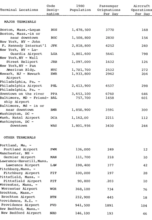
TABLE 2. NORTHEAST CORRIDOR AIRBUS TERMINALS, POPULATIONS, AND OPERATIONS PER DAY

Terminal Locations Code Desig-nation 1980 Population Passenger Orignations Per Day Aircraft Operations Per Day MAJOR TERMINALS Boston, Mass.-Logan Boston, Mass.-in or near downtown

New York, NY - John

F. Kennedy Internat'l

New York, NY -

La-Guardia Airport

New York,NY - Wall

Street Heliport

New York,NY - Pan

American Bldg. Newark, NJ - Newark Airport Philadelphia, Pa. -Philadelphia Airport Philadelphia, Pa.

-downtown on the river

Baltimore, MD -

Friend-ship Airport

Baltimore, Md - in or

near downtown Washington, DC

-Wash. Natnl Airport Washington, DC -downtown OTHER TERMINALS Portland, Me. -Portland Airport Manchester, NH -Gernier Airport Lawrence-Haverill,Mass. Lawrence Airport Fitchburg,Mass. -Fitchburg Airport Pittsfield, Mass. -Pittsfield Airport Worcester, Mass. -Worcester Airport Brockton, Mass.-Brockton Airport Providence, R.I. -Providence Airport New Bedford,

Mass.-New Bedford Airport

BOS BOC JFK LGA JRB NYC EWR PHL PPA BAL BMR DCA WAS 1,478,500 1,508,800 2,818,800 3,801,600 1,097,000 1,701,700 1,933,800 2,413,900 3,653,100 757,700 1,850,900 1,162,00 1,801,956 3770 2830 4252 5641 1632 2532 2942 4537 6760 1458 3591 2211 3430 249 218 377 197 .203 734 445 1891 168 154 240 798 126 272 204 298 646 601 300 112 244 104 PWM MAN LAW FIT PIT WOR BTN PVD NBD 136,000 111,700 198,400 100,000 90,800 368,100 232,900 941,500 146,100 193

-8-TABLE 2. CONTINUED Terminal Locations Code Desig-nation 1980 Population Passenger Originations Per Day Aircraft Operations Per Day Reading, Pa. -Reading Airport Harrisburg, Pa. -Harrisburg Airport Lancaster, Pa. -Lancaster Airport

York, Pa. - York

Air-port Trenton, NJ - Trenton Airport Atlantic City, NJ -REA HAR LAN YRK TRE Atlantic City Airport ACY

Wilmington, Del.

-Wilmington Airport WIL

Washington, DC - Dulles

Airport DUL

Richmond, Va.

-R. E. Byrd Flying Field RIC

Newport News - Hampton

VA - Civil Airport PHF

Norfolk, Va. - Norfolk

Airport ORF Springfield, Mass.-Springfield Airport Hartford, Conn. -Rentschler Airport Hartford-Springfield -Bradley Field Waterbury, Conn. -Waterbury Airport

New London, Conn

-New London Airport

New Haven, Conn.

-New Haven Airport Bridgeport, Conn.

-Bridgeport Airport

Norwalk, Conn. - SW

of downtown near water Stamford-Greenwich, Conn.-Between Stamford

& Greenwich near wat.

New York, NY -

Teter-boro Airport Long Island, NY

-Mitchell AFB (abandoned) Islip, Long Island,

NY - MacArthur Field

East Quogue, Long Is.

NY- Suffolk Cty AFB

East Hampton, Long Is.

NY - Airport

Scranton, Pa.-Scranton Airport

Wilkes-Barre, Pa.

-Wilkes-Barre Airport

Allentown, Pa. -

Allen-town Airport SPR HFD BDL WBY GON HVN BDR NWK SGC TBO MIT ISP EQU EHM AVP WBA ALL 667 1037 814 132 108 694 635 509 319,500 431,300 391,900 329,900 357,900 239,600 631,200 776,900 633,000 570,500 972,500 636,100 693,700 182,000 250,300 254,700 416,600 499,600 196,800 796,200 1,023,200 1,627,200 417,700 292,200 1337 1501 1246 1107 1868 168 140 1336 1431 380 506 535 804 908 331 1301 1555 2508 741 628 266 403 634 1259 216 126,100 194,200 271,900 621,700

-9-nation

C is chosen such as to cause a specific peaking of the d

variation with distance (e.g. for 200 miles C

=

.007,

for

100 miles, C

=

.015).

The value of

is taken as 2.0.

This data is not a prediction

-

it is a hypothetical

pattern of demand generated to examine in detail the problems

of producing a schedule or timetable by computer, and to

allow some idea of desirable vehicle sizes, terminal sizes,

number of operations, vehicle and terminal utilizations, etc.

to be obtained. Both the scale and the pattern of demand

can be changed in order to examine the sensitivity to such

changes of certain operational information arising from the

system schedule. It is expected that detailed projections

of Northeast Corridor demands from other Department of

Com-merce studies will become available at some future date. As

a result of the studies reported in Reference 3, a second

pattern of demand has been generated with the peak of the

pat-tern shifted from 200 to 100 miles.

See Figure 2. Such a

shift assumes that the air system will have a larger share

of the total travel market, particularly for trips below 200

miles.

Since the previous results indicated appreciable time

savings, and lower costs, this shift in demand was indicated

in generating a second demand pattern.

-10-50

40

DEMND MODEL 2

30

L

CL F-J20

_

C0.007

DEMAND MODEL

1

10 -

D

-3xlO -7 x

e- (Cd)

2

P P2

d 0.4

0

1

1

1

11

0 100 200 300 0

DISTANCE ,d, (Statute miles)

N.E. CORRIDOR DEMAND FUNCTION FOR AIRBUS TRAVEL

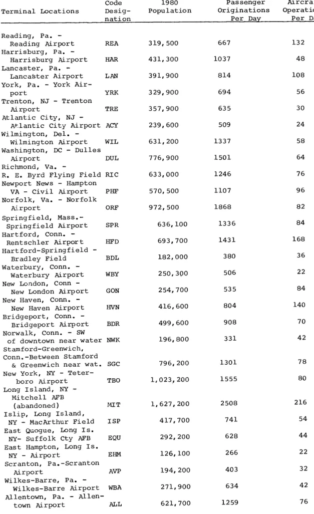
The demand data is given in Table 3. It is a 50 x 50 matrix called the D2 matrix, with a subscript 2 to indicate

the second demand pattern. The data is 0 & D data (origina-tion and destina(origina-tion) where the matrix entry dij gives the number of trips per day from point i to point

j.

As is generally true for passenger traffic (but not cargo or

freight), the matrix of Table 3 is symmetric, where di =

d . The diagonal consists of zeroes, and the sum of any

row represents the number of trips out of a given point, i. Similarly the sum of any column represents the number of trips ending at a point

j.

Table 2 gives the number of passenger originations for each station for the D2 matrix. The second demand generates 27.7 x 106 passengers per year

compared to 16.7 x 106 for the first demand matrix, D₁.

Each entry, dijs represents a best estimate of the mean or average of daily travel demands on the system over some period

such as a peak month or season. Daily demand varies from day

to day in recognized seasonal and weekly cyclic patterns,

and is a probabilistic or stochastic variable. In this study,

dig represents the mean of such variations over all days of a peak month or season, and a system load factor is assumed

later to be 60% to ensure that daily demands above the average

-12-TABLE 3 - DAILY TRIPS BETWEEN CITY PAIRS - SECOND DEMAND

J ci 02 00 < z j C 4 M j a 4 mj w Z m- X0>- 2 L F Co IL cc If 0 0 x uk u x 2a3 U D 4 0 0 4 0 > - I 2 M 4 ._j < 0 a. - 0 t 0 2 3 a y 1 o I 0 2 < - t 2 - x. 4 w > n ; 0 x

-c o co I ca > z a. 3 a I F r a r 3 0 a o , 0 - w m I 3 v x < I 3 3 1- 2 0 2 a a. 4 o 2 - ww a- - J

DCA 691ii i 5T T i 88 329 47 43 5o 8 T 6 34 64 9 1813331449 131235 54 44 26 26 11i 32 95- I9 22 203 131 1 e 497 78 38 2419{

_C

56197 2934 5 *[16 221 30 13 1 21

DUt 32 o 92 712319160o69 i 9 34 L 85 42% 36 61 I7I 2i9 f1 47| 21 94H 37 92315" 13236 255 32 912 25 16 59 4 3 9 8 6 2

-AL 1 2 9 i 4 ₈1 32 _1os7N 26 26 55 1 ₁ 33431I j 920 309 91 242 37 6344 17 48 217 412 3 0 7~ 6 -1 304 ₁ 140-_ 6, 31, 50 18 6 _ 32 9 8 6 - 5 2-1 F512

is 1 so if 6 89 29 _{4 4 6},603 ₁₇i 290 86 721 43; 40 3 1226 2 161 268,107 69 6 27'33 33. I 22 7

80C 9 1 191 35 52 44 52 962! 39j951 29 459 621 17 307 88 73, 44 40 111 3 27 2 i750" 513! 6442269 i1 2 1 22 23 6 7

MAN _MA2i 24 aI f _{3 7 5}

31

1f-3 -1 5-331 9 1 23710 55170i1431722718- 0 6 3 ' 12 53 ~~3

2-WOR 4 I 18-3-, 62I3 16 01 1 1 21 16 9 8 1 9 5 5 72 27 18 132 1 6 7 3 8 2 5 6 101 55

N80 9 I o33; S5 3 3 ii I i 9 24 6 7 127 1 6 1 l4e 3 12 4 3 1 s 5

WVL 224 30 87 1 5 8 6 1 4 2 1 i 7 7

_ v - 4 60 2221 35293 594 12 49IO 1 0 7 1 1 52 40! -7 148i1 2!95I 3 I0I I3i hiw 387tI4-22 s2 2' I6 i -5 I9 I

WIL 7 IV I4i 4 3if529 6il 24 53 6 32 2 2

TR E7 7 4 6 4 REA T 1 7 4 7 900 8414 0 69 1 8 3 67 61 61 3 230 , 43 9 2 7 LAN 24 2 I9 0 21

Sl

1 2 7L 1 2 4 7 2 ,2 48 30, 8 12 5 4 4 18 7 R 4 Idi s 2 i

e1

8 4 s -- 8i_ WBA 9 I I 6 ~5 4I I9 18 5 52 15 5 6 6 3256 6 4 5 0 7 1 6 f SPR I I i4 4i li ti Ii ii 2 s 12e 29 6l [2i2- 0 e- 1 4 3 - - 12 1 1i 040 12 2 i 5 4 -eDL ] Is'l ie 3 7 3 475 4 7 JFK: 6 So 8 9 2 1i-6 4c4 1 So 6 -4 - --4- 1 -- - 1 291 - 36_1- f _ JR0 _N 6 15 23 414 923 2 38 30 9 I 2 60 61 2 _{9 80 1211} 3 57013 278 81 5 2 6 324 11 28 46 910 2i 86i363 5 1 WBy _N I ₉₁ 4 1 _{of 3} 62 ₅ 5332 '

e

6472 5 4 7361 4 9 12 7 1 6 216 8 1 5 1 6 3 4 HFD 32 2050 2 14 28 50 2 9 1 0,9 11'7 2,4 2 2:2 9 1 4 13 29 70 7 0 1 6 ! 4 1 -f I

j0

Ii ! 1f I-~ I i R 7-2 - 2T01 8 214 ACY5 6 41! 3 457 2 102? 3 1 1 T1 2 2 BMR1 59 23 41 7 t 15 31 3 1211 48 9 1 8641 4017 49 3 5 9 3 34 4 wFs r08 ii 6 s0 h r 4as' 522R 1 52 5 134 7 1102146.273 62 4 71 li 3, 3241 72i 39 TBO 1 12 8 T 2231 2 -69N 02

f8

2 21 331 12 457' 195 19 84 5 6 5 476 4 9 R 3

[

3 6 21 252 69 2 1 1 3 1 24 7 1541112

EW Ii 1 1 I28 i 7-_1 58 1- 3i- i l-il-7 11 65 10 5 41 71 22 24'- 21 4- 3

WRY 2 4 9 2 4 2-1 5 41 3 24 1 41 2 9 13' 2 I 2 3 15I 7 6 1 1

PPA 5o 64 3 149 35626

-

I

I tT 16 -ii - 9 I 3i 7 -i

4--WY

1 1

9 7 I3 40 45 1 3 0323 018 20 937.7301 129.94 44j 8 4 0 5 9 3

s

WAS 1 I4 _{18 19 Il 119 79Tl f l j 13---I-I W}

_~

₁₁ 35I _i 22759 _{11 31281}32 22 15 4,,

MC 4 9 5 1 ,2 13 2

NW 24

5-2-III I

I23.2-

1 08 149 93 7,3 81 1 61 84 -7 78I49 29 8 2 3

NYC Iil2- 121: -8 1 71 12 56 4 4 73 i4.-i.IiI C9R4,-i

NRYCI1 - 1948197 16244 88j 6313714 i 425, ii i3 OR I I I4 10 357 I~ j~ I Ii I17 14' RIC 681 24 11 441 ' I 41141215 621 9 43 1359 P M

I

2 4 PHI' I 20 1040 10 129 14 6 5 4 10 8 YRK -t 14 I iI- 84 9 99 49 3 580 665 SGC 1 10 22 9 ' ' NWK r 2 5 2 3 - 5 90 129 49

II

I

HtI

I~

1~

3-4519

F

IT

2 BTN T LAW F J V 0 Z :

I

Z I q I _: , In , o- o w n <Q m LA -

1

11 1 1

0 I j4 . 0 v It 1, 1 > L a- X > ' LJ 1I KL 01 f .9 1 J1 In m ml 2n 2 0 .o 4 LU X 2 j m~ A - 10 a In._

are accommodated. Variations of demand with time of day

are accounted for by choosing departure times in the

time-table construction.

The demand data assumed available here is similar to

that obtained by the CAB in its present method of sampling

ticket sales and recording the 0 & D flow by all airlines

between various points. If the airbus system were operating

with a computerized reservation system or more precisely a

management information system, such data could be continuously

gathered and made available for any time period. Future

pro--jections could then be based on this data in planning

sche-dules for future time periods.

Often, a more detailed description of demand can be

available for purposes of schedule planning. For example, the

weekly cycle of demand could be studied with the goal of

providing different daily timetables, or a semi-weekly schedule;

or, competitive factors between companies or between modes

could be available. No such complexities have been allowed here. The abject has been to provide some idea of the

geo-graphic distribution of daily demands in order to determine

the frequency of service pattern for the assumed system. This

process will be described in the next two sections.

III. PASSENGER FLOW PATTERN

The demand matrix, D, gives the number of trips per day from City A to City B. Unless the system is providing

direct non-stop service between all city pairs this will

not be the totality of passengers using the route A-B since

other "through" passengers will use the route in going

X - A - B - Y. For 50 cities there are 2450 possible

non-stop services, but not all of them will generate

suf-ficient demand to warrant non-stop service. This can be

seen by examining the D matrix. On most airline systems 2

only about 15-20% of such possibilities are economically

attractive, so that there is a substantial percentage of

through passengers on most direct services.

It is necessary to have some method of determining the

passenger flow patterns for a given subset of non-stop

services. The total passenger flow (non-stop plus through

passengers) then determines the daily number of non-stop

seats required, or the frequency of daily non-stop service

required for a given vehicle seat size and load factor.

This process is sometimes called detennining the frequency

of service pattern for the system. Lesser routes are dropped

to zero frequency in favor of higher frequencies else-where.

This section will describe the techniques used to produce a passenger flow pattern (the F matrix) given the subset of routes to be serviced. We are interested in matching available seats/day against passengers/day on each route to be serviced in order to obtain the frequency pattern (the N matrix)in the next section. In other words, we are trying to determine on a system wide basis a balanced

allocation of available seats to the geographic patterns of demand.

A multi-commodity network flow computation is used

to re-route the passengers from X to Y via the shortest

routing X - A - B - Y. Initially, an assumption has been

made that least distance can be used as a criterion for determining the "shortest" routing. It is probably a good representation of least time when the frequency of service on all routes is fairly high, and the model can be exten-ded (as shown in Appendix A

)

to be precisely least time when the time of day network and a discrete timetable are

used. It is assumed that a passenger will use the services which have the earliest arrival at Y, and that the indirect

routings will not have an effect on the D matrix demands.

Neither of these assumptions can be rigorously defended.

In the airbus system, it is planned that knowledge of the

earliest available arrival at his destination via indirect

routings will be available to the passenger through the

system's computer, and that intermediate stops will delay

the flight only a few minutes. Both of these factors will

tend to make the assumptions more applicable to airbus

ser-vice than to present airline serser-vice.

Methodology for Determination of F Matrix

The methods used to determine shortest paths and the passenger F matrix are drawn from network flow

theory, and the theory of graphs. A fuller theoreti-cal understanding of these concepts can be obtained by reading Reference 4, and then Reference 5. A brief

explanation of the techniques will be given here. The computer program .sed was a modification of an IBM SHARE library coding by Dick Clasen at Rand Corporation for the "Out of Kilter" OKF algorithm of Ford and Fulkerson. This algorithm is applicable to large transportation network problems where the num-ber of arcs and nodes can be 4500, and 1500 respect-ively. _{Solutions give integer values of xij and are} obtained within 10 minutes of computation on an IBM 7094.

Suppose we have a network or graph G which con-sists of nodes (i,j,k...) and directed arcs (ij, jk,...) such that closed paths or circuits exist in the graph. With each arc ij, there are three associated scalar quantities;

lii = lower limit on arc flow

uij = upper limit of arc flow = capacity cii = unit cost of flow from i to

j

and the variable x.. which is called the flow of some

com-1J

modity from node i to node

j.

We wish to determine a flow X =

x..,

X. ,... such

that:

1)

1..

( x.

u..

Capacity constraints

1J 1J 13J for all arcs.

2)

(x..

- x

)

=0

Conservation of flow

(i., jk)

at nodes j.

3) x.. are integer values

1J

and which will minimize the total flow cost,

Z

=c..

.x..

arcs ij

This is recognizable as a special case of the general

linear program where a.. =0,

+

1, and is called the

transpor-1J

tation or assignment problem. It is widely applicable to a

variety of transportation or scheduling processes,

particu-larly since the size of the Out of Kilter algorithm and its

integer solutions allow practical problems to be solved. If

posed as a linear program, there would be 4500 variables with

9000arc equations for the upper and lower constraints and 1500

node equations.(i.e.a'matrix of 10500 rows and 4500 columns).

Since most of the a.. matrix entries are zeroes

(

matrix

den-1J

-19~

sities for this type of problem are typically 10 percent), the

labelling technique used by Ford and Fulkerson is far more

efficient than any variant of the Simplex technique. If l..

1J

and u.. are integers, we are assured that any feasible solution

1J

for X will also be integer.

Description of the Model for Passenger Flow

To use this technique, it is necessary to construct

a graph or network as a model or representation of the

pas-senger flow problem. Figure 3 shows a simplified network

representation of the model.

The subgraph of "city" nodes A, B, Ce.. and

"service" arcs [AB, BA, AD, DA, ... represents the

geo-graphic or service network of cities A, B, etc. and

non-stop services operated between cities AB, BA, etc.

If service between cities A and B is to be operated non-stop, then a pair of directed "service arcs" AB and BA exist in

the service network. In Figure 3 this pair of arcs is repre-sented as a solid line with both directions indicated by

arrows. Each arc has its cost (cij) value set to s, the

distance in miles between the city pair. Every service arc

has lii = 0, and u = 00 . Thus, there are no capacity con-straints on the flow in service arcs, and the value of the

flow, xij, will represent the number of passengers/day wishing

to use this service.

The arcs LAA*, BB*, etc. are another subset of arcs

called "disembarcs". Nodes [A*, B*, C*,... are called

-21-SERVICE ARCS

(0S

Bc

B

(

0

,SCE'

O)

DISEMBARC

N,

(0,D,co)

(dBAOdBA)

tI

_(d

0O

d)

~ DEMAND A

FIRURE3(a)

NETWORK FOR PASSENGER FLOW SOLUTION

TRANSIT ARC

IA

SERVICE ARCS FROM

OTHER CITIES

FIGURE 3

(b)

SERVICE ARCS TO

OTHER CITIES

DISEMBARC

MODIFICATION OF CITY NODES

station nodes. There is one disembarc for each city. Their values of lii and u are 0 and 00 respectively as for the

service arcs, and the cost for these arcs is D, the diameter of the service network. A diameter is the longest track or

elementary path in a network, and this value is placed upon these arcs to prevent flows from disembarking at an inter-mediate station and travelling via demand arcs to their des-tinations. The value of the flow in a disembarc represents the number of people arriving at that station per day. It will equal the sum of the associated column of the D matrix.

From every station node [A*, B*, C*, ...

]

there is a subset of arcs called "demand" arcs. For example, from node A*, a demand arc exists going to all city nodes [ B, C,

D, ... ] . The cost on these arcs is zero, and both lii and

uig are set to a value representing the daily demand in pas-sengers/day between city B and all other cities. These demand arcs ensure that a flow x.. equal to the demand d exists in the demand arc, and necessitates a return flow via the shortest

path through the service network. For example, the demand

arc A*E in Figure 3 causes a flow in the service network back

to A and A* via either EDA or EFA whichever is shortest. The node conservation constraints cause all flows in the complete

graph to be circulations, or flows in a circuit. For an

n-city problem, there will be n x n-1 demand arcs. If the

demand is symmetrical, some modifications can be made to

avoid repetition of demands. In this case, there are only

n x n-l demand arcs. 2

At this point, the multi-commodity aspect of the problem is encountered. Every x.. flow into a given city must be

considered as one commodity, xig, to prevent the flow x along the shortest path in the service network from being

exactly cancelled by the symmetrical flow, xji, along the

identical path in reverse order. A modification of the

labelling technique in OKF was made to remove the reverse labelling. In this way, an x.. value, once placed in the

network, could not be removed, and the return flow, x , uses the symmetrical forward path along the other member of

the service arc pair.

Since there are no capacity constraints on service arcs in this problem, the multi-commodity aspect can be handled efficiently within one run of the OKF code by solving for each city sequentially. The "Alter" option of the coding was used to impress new demands for the flow into the next city.

-24-The complete solution for a 50 city case takes around 10 minutes on the MIT IBM 7094 while in CTSS operation.

(Com-patible Time Sharing System).

Information Available from the Model

This modified algorithmic process will minimize the

total flow costs over the complete graph:

i.e. Minimize Z = c.. x s. x + x D

JIJ 13 ij _{i iji}

service

arcs disembarcs

But, since D = constant, and for any given demand the xij in

the disembarcs is fixed equal to the column sums in the D matrix, i.e., the total number of originating passengers per day, P. Min (Z) = Min s. x + P.D service 3 i] arcs = PM. + P.D m.in

The constant RD is readily calculated and subtracted from Z to get PM min. We are minimizing total passenger miles (PM) in the network, and every individual passenger will be

travel-ling his shortest route since there are no arc capacity con-straints.

The average passenger trip distance is then:

PM

p PV

-By a simple trick of splitting the nodes

A,B,C...

L

into two parts separated by a "transit" arc, as indicated

in Figure 3b, further information can be obtained. For

example, node A becomes two nodes:

IA which receives all

service arcs from other cities, and OA which starts all

service arcs out of city A. The transit arc

IA, OA}

has a flow which is the number of people passing through

the station on their trips to other destinations.

The number of passenger departures per day, PD, is

obtained by summing xi

in the transit arcs and adding P.

PD

=

x

+ P

transit arcs

From this we can obtain the average hop or non-stop

distance for both passengers and vehicles:

-~

PM

D

=

-H

PD

-27-As well, the frequency distribution of hops can be

obtained. If we categorize service arc distances, then

the sum of x.. for arcs in each category are an

indica-1J

tor of frequency.

The average number of hops/passenger is

-- PD

P

The most detailed information available from each solution is X itself. For the service network X = (x. for all ij in network), is precisely the F matrix which

gives the number of passengers/day using each service.

It is possible to obtain the indirect routings and the number of passengers per day on them. This has not

been carried out as yet. That information could be useful

in constructing flights consisting of a series of flight segments by the same vehicle at a later stage in the schedule construction process.

-28-The Network Models for the VTOL Airbus System

For a system serving the 50 shopping points shown in

Figure 1, a model was constructed. There are 2450 possible

demand arcs which obtain d.. from the demand generation

1J

program.

There are

50 disembarcs,

and

50 transit arcs,

and

somewhere between 200-500 service arcs. The distance

costs,

sig,

are the great circle or airline distances used

in the demand program. The value of D was set at 1000 miles.

Several solutions were obtained for both D and D2

demand matrices, using different service networks. The

service networks were selected on two criteria. The first

was geographic where each station was connected to two of

its closest neighbors by "basic" arcs.

These basic arcs

were members of every service network.

The second criterion was either demand,

d..,

or

pas-1J

senger

flow,

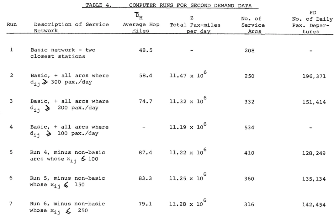
Xi

Table 4 describes the sequence of runs

for the second demand, and indicates how the various service

networks were selected.

A strategy of including arcs of

lesser 0 and D demand dii was followed in the first

four runs,

and the frequency of service pattern determined as explained

in the next section.

Adding more and more non-stop services

dilutes the service to the point where a small number of

TABL 4. COMUTE RUS FO SEONDDEN~flDATA Description of Service Network DH Average Hop iailes Total Pax-miles per dayv No. of Service Arcs

~

PD No. of Daily Pax. Depar-tuires

Basic network - two

closest stations

2 Basic, + all arcs where

d. > ..,300 pax./day

3 Basic, + all arcs where

d

>

200 pax./day

4 Basic, + all arcs where

di j, 100 pax./day

5 Run 4, minus non-basic

arcs whose xij

4

100

6 Run 5, minus non-basic

whose xij ( 150

7 Run 6, minus non-basic

whose xij ( 250

58.4

74.7 11.47 x 106 11.32 x 10 11.19 x 106 87 ,4 83.3 79.1 11. 22 x 10 6 11.25 x 10 11.28 x 10 Run 48.5 208 250 196, 371 332 151,414 534 410 128, 249 360 135,134 316 142, 454 TABLE 4. n r d y Ar s

passengers per day were using various lesser services. The

strategy then became that of dropping service on these low

density routes and asking these passengers to proceed

in-directly via routes which enjoyed higher passenger flows.

Basic service arcs were always retained so that no station

could be isolated. Passenger flows on basic arcs is often

very low, and can be used to consider dropping the station

from the system.

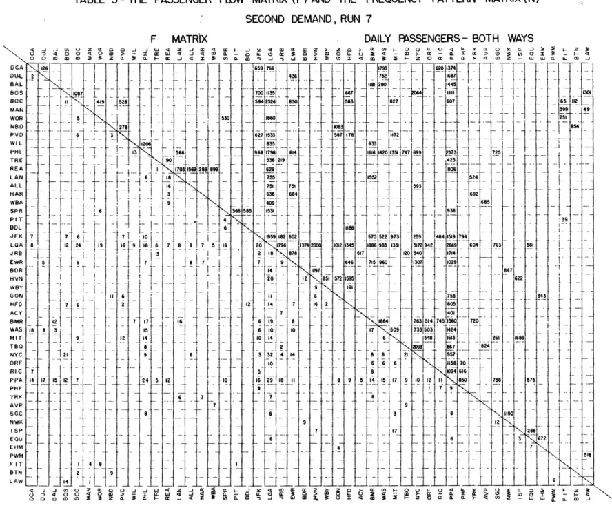
-31-TABLE 5 - THE PASSENGER FLOW MATRIX (F) AND THE FREQUENCY PATTERN MATRIX (N)

SECOND DEMAND, RUN 7

00W 01o e 2 2 a W OCA 126 SAL SOS 1087

L

SOC 4 141 2 5 MAN F1l 4 WOR 5 NBO 278 P t 3

~

PHI

L

14

TRE REA WA

L

1

SPR 6 PIT SDL -T JFK 7 7 6 7 LGA 8 12 24 9 16 9 E WR 15 9 HVN WBY GON 6 11 6 HFO - 7 6 21 A C YI BMR 12 7 WAS 8 I

ij

NYC 2 ORF

RIC 7

PPA 4 17 15 12 7

1

PHF 1 YRK AVP ISP EQU EHM PWM F

IT1

4 8 BTN 2 9 LAW 14 L F MATRIX x m w1 4 4 W a. I- 4 566 90 1703 159 288I899 6 3 I 10 1 6 3 7

24 5

8 14 1 -J 0 () .7 a 0 0J 4i 1*3 Io :* 40 04 0 0>'i a a0a1w0 0 W 3 2 z (

I.l-16

2

1-8 7 5-, 6 t7 7 !a a-4 4 0 a) w. z 659766 436 700 1135 594 232 830 L 530 18601 62711533 968 1798 614 538 219 .62? 755 751 751 t 638 684 66 585 1531 463 6 959 182 602 16 20 1796 1374 201 2 86 878 7 9 4 1 97 0 - 12 851 9 7

12 14

7

16

2

7 6 _19 8_ 6 1 101 10 14

3 32 4

14

10 5 10 16 29 18 11 7 6 a i , J~ 4W 0m Z>

DAILY PASSENGERS- BOTH WAYS

1 0 >- m (n 0 2- 0 IL LWx >4 u . 0. a I z 0 IL 23 4 - W M- M r 0. X~ > 0 .> 0 an I ': 1: 1- 4 0 m 4W . W 1- 0 m a 0>1 4 0 z - d us mi IL 04 17991] 752 1181 2801 667 583 j827j

183-587 78 1172 633

k

I881

570 522 9731 1012 1345 1886 983 1331 617 646 715 960

572

15951

-61 1664 1 509 6-. 6 6 6 8 -8 9 -5 14 15 17 1 4

<F

T Liisj

7-I

---

1

-1 620 14

f1687.f

11 144 2D64

lt

607 f

8

9

9

37

3

f_

7

2

5

-24

692 936 259 14841519 5172942 6 i

120

340

₇₁₄

1307 102$ L 805

401

763 514 7451138C 733 503 1142 54 63 763 261

171-]

I--I -k -.1-. 2093 867 824 2957 --70 1094 616

9

0 12

850 758

575

1 9 288

6

1672

7

2

LI

I ii r

44*o . W I DAILY FREQUENCY - ONE WAY

65 1121 399 49 75 854 39

18

m--N MAT RIX

Typical Results

Results from the final run for the second demand are

given in detail in Table 5. Entries in the upper half of

the matrix are xi= passengers per day using service ij.

Other interesting results are given below

Total pax-miles/day = Z = 11.28 x 106

Total Passenger Trips/day = P = 76000

Total number of Passenger Departures = PD = 142,454

Average Passenger Trip Distance = Dp = 148.5 miles Average Hop Distance = DH = 79.1 miles

Average No. of Hops/Passenger = 1.91

The distribution of hop distances is shown in Figure 4,

compared to the distribution of city pair distances for the

50 stopping points.

100-NORTHEAST CORRIDOR

50

100

INTERCITY AIR

200

300

400

DISTANCE -N. MILES

DISTRIBUTION

OF INTERCITY

DISTANCES

(ALL CITY PAIRS)

50

100

200

300

400

VEHICLE HOP DISTANCE - N. MILES

DISTRIBUTION

OF VEHICLE

FLIGHT HOPS

FIG. 4

-34-80

60h-

40[-VTOL AIR SYSTEM

T

20

0

FIG. 4

(a)

a. 0

z O

00 QW

a3-z

OL

0

FIG.4 (b)

IV. DETERMINATION OF THE FREQUENCY PATTERN

Given the expected number of passengers/day using

a given route, an estimate of the desirable number of

ser-vices or direct flights/day can be obtained using vehicle

seat size and an average load factor established by

plan-ning policy. If we let

N

be the number of flights/day;

N.

Xj=ij < S . LF

where x = daily passengers from i to

j

- one way

S = vehicle seat size

LF = desired average load factor

< >

signifies rounding off to next highest

integer.

At the present time, it has been assumed that there

is only one vehicle size (80 passengers), and that for planning

purposes an average system load factor which should be

achievable is 60%. Other combinations of vehicle size

should be studied since within the present models there

are indications that a smaller vehicle on the low density

routes should be used to increase daily frequencies of service.

The average load factor of 60% is chosen to allow for

monthly and weekly cycles of demand, and to account for the

-35-fact that daily demand is a probabilistic variate from day to day. When a fixed seating capacity is matched against

the average of a probabilistic quantity, a capacity margin

above the average load is required to ensure that the above

average loads can be carried.

The time of day cyclic variations can be accounted for

in two ways: allowing load factors to vary with time of

day, and by bunching departure times at the peak hours.

Both methods are discussed in the next section.

It is assumed that a daily schedule will be established

for the period of the demand estimate. If more detailed

information were available regarding weekly variations in demand, considerations could be given to such things as a

semi-weekly schedule or special schedules for Saturday, etc.

Typical cycles of demand are shown in Figure 5. Similar

in-formation can be generated and estimated by the management

information system for the Airbus system.

It has also been assumed that there is no information

on competitive or marketing considerations which would

dif-ferentiate one route from another. Normal domestic airline

competition causes frequencies to be added by competing

air-lines to the point where marginal revenues tend to equal

marginal costs. As such, a variation in breakeven load

-36-factors with length of haul arising from the differences

between fare and cost structures causes varying market

load factors in competitive markets. It has been assumed

here that fares are proportional to cost, causing equal

breakeven load factors on all routes, and allowing the

planned load factor to remain constant for all services.

In this manner, the allocation of seats/day to a given

service is directly proportional to the estimated number

of passengers.

Given other situations such as the present

airline system, different assumptions and allocations of

seats/day would be made using suitable marketing

informa-tion.

No such information exists for this study.

The frequency pattern, or N matrix, corresponding to

the F matrix is given in Table

5

below the diagonal.

It

assumes an 80 passenger vehicle at 60% load factor, and

is symmetric. The entries are the number of one-way flights/

day for each service.

It is interesting to note at this

point that the N matrix of Table 5 has 2996 flights/day

which is 2-3 times as big as the largest airline schedules

in existence today.

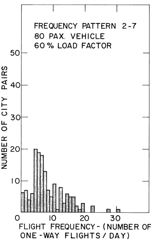
A frequency distribution of the number of one-way

non-stop services/day is given in Figure 6 for this N matrix.

The average value is

9.5 non-stop flights per day, and the

-37-FREQUENCY PATTERN

80 PAX. VEHICLE

60%

LOAD FACTOR

10

II

h l

[1

...

20

2-7

30

FLIGHT FREQUENCY- (NUMBER OF

ONE -WAY FLIGHTS /

DAY)

FIGURE 6

DISTRIBUTION OF FLIGHT

FREQUENCY (NON-STOPS)

-38-50

k-

4&F-0

w

m

z

30

20k-l

Ok-IlL

,..a %-.V.. 4r.. 4% T -, . ,

_a,

distribution indicates that there are many routes below

this value.

There are, however, a significant amount of

one-stop, two-stop, etc. indirect services on most routes

which should also be considered in determining the total

frequency of service.

The routes below 5 frequencies per day indicated in

the distribution are all "basic" services retained to

keep certain cities in the system. Also, examination of

the total system effect of dropping such cities can be

easily made.

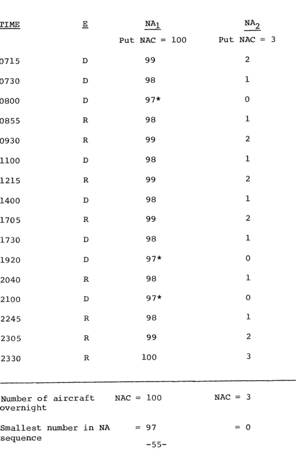
The number of operations per day for each station

can be obtained by summing the row and column of a complete

N matrix. The row sum represents the number of departures,

and equals the column sum which is the number of arrivals.

Totals for run 7 are given in Table 2 for all cities. The

largest station for this pattern is Laguardia airport with

798 operations per day. This would indicate use of larger

aircraft in Laguardia Service, or the establishment of

another terminal in the New York area. Similar considerations

would apply to the downtown Philadelphia site which has 646

operations per day. With the computerized methods used in

this study, new sites would be chosen in such areas, and a

new passenger flow pattern determined using a revised

estimate of demands between all stations and the new

sites. The N matrix or frequency pattern, and the new

number of operations/day per station are then quickly

tabulated.

-40-V. TIMETABLE CONSTRUCTION

Having determined a frequency pattern for all

non-stop services, the next step in constructing a timetable

or schedule plan is to assign departure times for each

of the N.. services on every route ij.

Given a departure

1J

time for a flight from i to

j,

and knowledge of the trip

duration or block time, the arrival time at

j

is

deter-mined. The set of departure and arrival times, properly

ordered for every station, constitutes a timetable

des-cribing in explicit detail the transportation system.

A computer program has been written to construct an

initial timetable given as input at this point three sets

of data:

1) the N matrix, or frequency pattern giving

Nij;

2) the A T matrix describing block times of ij;

3) data describing the daily variation in demand, d. (t),

fyJ

for every city pair.

-41-Determining Suitable Departure Times

In the absence of detailed information about daily

variations in demand for the hypothetical 1980 Airbus

System, two demand variations were assumed. A flat

dis-tribution from 0600 to 2400 hours, and an extremely peaked

distribution descriptive of Eastern airlines shuttle

de-mand on a Friday. These were considered as extremes, and

that the daily variation would lie somewhere between them.

These daily patterns were chosen after examining a

variety of patterns from various sources. The daily

traf-fic patterns for Northeast airlines, for all days of the

week and various months of the year were available.

Traf-fic patterns reflect passenger demand modified by the airline

schedule, and the peaking was much less severe than the EAL

shuttle pattern used. There were wide variations in

pat-terns at different times, on different routes, and from

day tD day. The number of aircraft operations per hour

at various Northeast Corridor airports was examined for

various periods to see the daily pattern as reflected by

Airline schedules, etc. Again the patterns were less peaked.

-42-MONTH OF YEAR

I

|

|

|

I

@

J

F

M

A

M

J

J

A

S

O

N

D

Month of Year

- 1965 Total,

US Domestic

DAY OF WEEK

1 .4i

i

i

i

i

i

1.2

0.8

0.6

0.4 M T W Th F S Su

Day of Week -NE Airlines,1964

HOUR OF DAY

2.0

-

t-riday

1.6

1.2

-0.8

0.4

0

2

0

2

4

6

8

10

12

14

16

18

20 22 24

Hour of Day - EAL Shuttle - Friday

TYPICAL AIRLINE DEMAND VARIATIONS

-43-1.2

1.0

[

-I

I I

0.9

0.8

0.7

0.6

2.4

FIGURE 5

Finally, detailed passenger and aircraft information for one day's operations at New York JFK Airport were examined to see the hourly variations in passengers and number of

seats for domestic services. Load factors were

substan-tially higher during peak periods,, since the passenger distribution was more peaked than the aircraft distribu-tion.

It is not possible or desirable to present all the information on daily variations examined. A sample of typical airline traffic variations is shown in Figure5

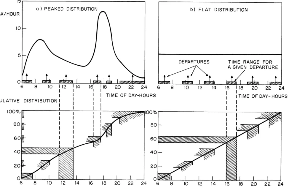
The method of choosing departure times for N.. flights in ij service is explained by Figure 7. The two distri-butions of the arrival rate of passengers (or of the proba-bility density of passenger demand) are shown in the upper portion of Figure 7. Below them are the cumulative proba-bilities of demand obtained by integrating the probability density distributions or arrival rates. It goes from zero to 100%, and represents the cumulative number of passengers arriving during the day. The uniform arrival rate gives a straight line cumulative from 0600 to 2400, while the

peaking shows much steeper slopes during the peak periods.

-44-The rationale first used to select departure times

was to divide the daily load on a given route equally

amongst N.. departures by dividing the vertical axis of the cumulative distribution into N.. equal segments.

LJ

The departure times could then be found by reading the

corresponding time from the horizontal axis. However,

because of the optimization process described in the

next section, this was changed such that a range of

times was selected for each departure in a similar

manner. Thus, the vertical axis was divided into 2N. -l

parts so that N.. departure ranges could be selected.

1J

The departure time was placed in the center of each range

to form an initial timetable.

This is shown in Figure 7 for both distributions

when N.. = 6. The vertical axis is divided into 13

seg-1J

ments, and the departure ranges are shown by the shaded

bands. For the uniform or flat distribution, the

depar-tures are equally spaced. For the peaked distribution,

the departure times tend to be bunched at the peak hours,

when their ranges are also much reduced. There is always

a gap between departure ranges such that two successive

PROBABILITY DENSITY OF PASSENGER DEMAND 15-%PAX/HOUR 10 5-6 CUMULATIVE 100% 80 60 40 20 0 6 b) FLAT DISTRIBUTION

DEPARTURES TIME RANGE FOR A GIVEN DEPARTURE

| | | |

6 8 10 12 14 16 1 18 20 22 24

I O

I| TIME OF DAY- HOURS

8 10 12 14 16 18 20 22 24 6 8 10 12 14 16 18 20 22 24

FIGURE 7 METHOD OF DETERMINING DEPARTURE TIMES

departures for the same destination will always be separa-ted even when they are moved to the closest end points of their ranges.

The initial departure times chosen by this method are symmetrical in that flights leave both i and

j

for

j

and i respectively at the same time. Furthermore, there will be departures at precisely these same times for every city pair with the same number of daily flights, since the daily variation in demand is used for all city pairs. This symmetry is partially destroyed during the optimization process of the next section.

There has been no consideration of continuing, through flights at this point. They would be constructed after

seeing the connectivity of the flight hops after the op-timization process of the next section. Similarly, there

has been no consideration of interconnections between flights, or between other modes of transportation. The possibility of competition (a critical factor in choosing times for airline schedules) has not been considered here. All these

considerations would be introduced at a later stage if

per-tinent information were available. Notice that the departure

times are chosen from the same daily variation for all routes,

representative of 0 and D demand, not indirect demand through a station.

The two daily variations in demand, and the resulting choices of times represent two extremes of the problem of peaking. The choice of departure times from this method also represents two philosophies of matching ser-vice to these demand variations. It is possible, for

example, to choose times uniformly throughout the day, and allow the load factor variation to handle the peaking. An average load factor of 45% would give peak load factors of 100% during the 5-6 pm peak for example. This approach avoids bunching of departures in order to maximize

utili-zation, and accepts lower average load factors. However,

the low load factors on off peak flights causes proponents of this approach to comment on sensitivity of loads to timings, and to move flights towards peak times whenever possible.

The second philosophy is to maintain load factors on individual flights, and to bunch departures at peak times. Load factors are higher at the expense of aircraft utili-zation, and the lower utilizations cause movement of

flights away from optimum market times in order to make connections which ensure better vehicle usage.

-48-The results in either case begin to resemble each other, and it is expected that the two results obtained

here will bracket a reasonable schedule.