Developing a potential retinal OCT biomarker for local growth of geographic atrophy

Developing a potential retinal OCT biomarker

for local growth of geographic atrophy

The MIT Faculty has made this article openly available.

Please share

how this access benefits you. Your story matters.

Citation

Yu, Yue et al. “Developing a potential retinal OCT biomarker for local

growth of geographic atrophy.” Biomedical Optics Express, 11, 9

(September 2020): 399506 © 2020 The Author(s)

As Published

10.1364/BOE.399506

Publisher

The Optical Society

Version

Final published version

Citable link

https://hdl.handle.net/1721.1/129545

Terms of Use

Article is made available in accordance with the publisher's

policy and may be subject to US copyright law. Please refer to the

publisher's site for terms of use.

Developing a potential retinal OCT biomarker for

local growth of geographic atrophy

Y

Y

,

E

M. M

,

S

C

,

Q

R

,

P

J.

R

,

N

K. W

,

J

G. F

2_{Department of Electrical Engineering and Computer Science, Research Laboratory of Electronics,} Massachusetts Institute of Technology, Cambridge, MA 02139, USA

3_{Bascom Palmer Eye Institute, University of Miami Miller School of Medicine, Miami, FL 33136, USA} 4_{New England Eye Center, Tufts Medical Center, Boston, MA 02116, USA}

*_{jgfuji@mit.edu}

Abstract: Geographic atrophy (GA), the advanced stage of age-related macular degeneration, is

a leading cause of blindness. GA lesions are characterized by anisotropic growth and the ability to predict growth patterns would be valuable in assessing potential therapeutics. In this study, we propose an OCT-based marker of local GA growth rate based on an axial projection of the OCT volume in the Henle fiber layer (HFL) and outer nuclear layer (ONL). We analyze the association between our proposed metric and local GA growth rates in a small longitudinal cohort of patients with AMD. These methods can potentially be used to identify risk markers, stratify patients, or assess response in future therapeutic studies.

© 2020 Optical Society of America under the terms of theOSA Open Access Publishing Agreement

1. Introduction

Geographic Atrophy (GA), the advanced, non-exudative form of age-related macular degeneration (AMD), is characterized by contiguous losses of the photoreceptors (PR), retinal pigment epithelium (RPE), and choriocapillaris (CC) [1]. To date, there is no FDA-approved treatment that has been shown to effectively prevent, slow, or stop GA progression. In developing GA therapeutics, the ability to predict GA growth rates and patterns would expedite clinical trials by enabling stratification of patients on the basis of predicted lesion growth rates and the directionality of this growth.

Several prior studies have examined correlations between GA growth rates and metrics of lesion shape [2,3], structural impairment [4–14], and CC blood flow impairment [15,16]. These studies can be divided into those that correlated measures of global GA growth (i.e., disregarding the directionality of GA growth), and those that correlated measures of local GA growth (i.e., considering the directionality of GA growth). Studies of local GA growth patterns, the focus of this paper, have found correlations between local GA growth patterns and OCT-based biomarkers of structural impairment [6,7] but not CC impairment [17].

Motivated by the promising correlations between local GA patterns and imaging biomarkers of structural impairment, and in particular the results of Stetson et al. [6], in this study we develop a simple, OCT-based biomarker of local GA growth that is derived from a slab encompassing the presumptive locations of the Henle fiber layer (HFL) and outer nuclear layer (ONL)—which we term the HFL-ONL control (HOC) slab. As will be detailed, the HOC slab is designed in order to capture four different OCT features, each of which has been linked to GA growth: (1) increased HFL/ONL backscattering; (2) HFL/ONL thinning; (3) descent of retinal layers; and, (4) hyper-reflective foci (HRF). This study demonstrates a pilot assessment of the spatial correlations between HOC values along GA margins and local GA growth rates in a small longitudinal cohort

#399506 https://doi.org/10.1364/BOE.399506

Research Article Vol. 11, No. 9 / 1 September 2020 / Biomedical Optics Express 5182

of patients, introducing techniques that can be extended to larger longitudinal studies in the future.

2. Methods

The methods described in sections2.1–2.3,2.5, and2.7are similar to those presented in a previous study from our group [17], and so are summarized only briefly.

2.1. Patient enrollment

This study was conducted at New England Eye Center of Tufts Medical Center, Boston, and was approved by Institutional Review Boards at the Tufts Medical Center and the Massachusetts Institute of Technology. The study adhered to the tenets of the Declaration of Helsinki and complied with the Health Insurance Portability and Accountability Act of 1996. Written informed consent was obtained from patients prior to imaging. During a 3-year period from 2014 to 2016, patients with GA were enrolled in this study and longitudinally imaged. Each patient underwent a comprehensive ophthalmic examination, and eyes with other macular diseases, myopia >6 diopters and/or significant media opacities were excluded from the study.

2.2. OCT imaging

All eyes were imaged with a 400 kHz swept-source OCT prototype instrument at ∼1050 nm wavelength. The full-width-at-half-maximum (FWHM) axial optical resolution was ∼9 µm and the transverse resolution was ∼20 µm in tissue. Image acquisitions were performed with 500 A-scans per B-scan, 5 repeated B-scans per B-scan position and 500 unique B-scan positions per volume, corresponding to a 12 µm isotropic transverse sampling density. This protocol generates both OCTA and OCT data, although only the OCT images were used in this study.

2.3. Mitigation of artifacts

2.3.1. Motion artifacts

Orthogonally scanned (horizontal-fast and vertical-fast) raster volumes were acquired in each eye. Using a previously described motion correction algorithm, a single registered and merged volume was generated from the orthogonal volume pair [18–21]. This approach estimates the motion of individual A-scans using similarity between an orthogonal pair of volumes with a regularization condition. In addition to motion correction, this increases the signal-to-noise ratio by volume merging. Regions with data gaps, which can occur at the intersection of motion in the two orthogonal scans, were automatically identified and excluded from the analysis.

2.3.2. Vessel shadowing

Areas underlying large retinal vessels were also automatically identified and excluded from the analysis. We generated the large vessel mask by a median projection of the OCTA volume through the RPE. The projection range extended from Bruch’s membrane to 45 µm anterior in order to capture the retinal vessel OCTA flow signals that project onto the RPE.

2.4. Segmentation

For each baseline volume, the RPE and Bruch’s membrane (BM) were automatically segmented using a custom graph-cut based method (unpublished). These segmentations were manually inspected and corrected using a tablet (Wacom Cintiq Pro 24, Wacom Co., Ltd., Japan) for each OCT B-scan. Then, an RPE maximum contour was generated by computing the maximum OCT value within the ±18 µm of the segmented RPE. The rationale for using the RPE maximum contour, rather than the hand segmented RPE contour, was to reduce the dependency of our method on the particular grader performing the segmentation (different graders may define the

position of the RPE segmentation lines differently). Finally, the RPE maximum contour was smoothed along the horizontal direction using a Gaussian kernel (σ= 60 µm).

2.5. Lesion tracing and registration

An experienced reader manually traced the baseline and follow-up lesion margins using an en facesub-RPE slab formed by a mean projection from Bruch’s membrane to 340 µm posterior to Bruch’s membrane [22]. Fundus autofluorescence (FAF) images were consulted in ambiguous regions. Per the Classification of Atrophy Meetings (CAM), lesions were required to measure at least 250 µm in diameter along at least one lateral dimension in order to be considered as GA [23]. Margins from both baseline and follow-up visits were aligned by manually selecting a set of corresponding fiducial points and then registered using an iterative closest point (ICP) algorithm. To mitigate small tracing and registration errors, the baseline visit margin was forced (clipped) to be inside or on the follow-up margin.

2.6. HFL-ONL control (HOC) slab and projection

The HFL-ONL control (HOC) slab is comprised of the majority of the ONL and portions of the HFL. In general, the ONL contains photoreceptor cell bodies, while the HFL is composed of Müller cells and photoreceptor axons.

2.6.1. Computing the HOC slab

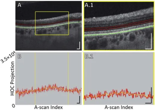
The HOC slab is formed by the mean axial projection of the baseline OCT volume through a ∼30 µm range, with the anterior boundary of the slab positioned ∼110 µm anterior to the segmented RPE, and the posterior boundary positioned ∼80 µm anterior to the RPE maximum contour (Fig.1). The slab position and thickness were empirically determined from a set of normal subjects, and their rationale is further described in the Discussion. Here we emphasize that the HOC slab was computed using the baseline, rather than the follow-up, OCT volume.

2.6.2. Excluding drusen and the central fovea

A drusen mask was formed using the separation between the RPE maximum contour line and the BM segmentation line. In particular, all regions with separations greater than 45 µm were considered to be drusen. This threshold was selected by qualitative assessment of our dataset, on the basis that it offered a reasonable balance between maximizing the amount of GA margin analyzed and minimizing the number of artifacts caused by morphological deformations. Regions of drusen were excluded, with the rationale that they alter the morphology of overlying retinal layers, complicating HOC analysis. We also excluded the central foveal region within a 0.5 mm radius, fovea-centered disk because there is a rapid spatial variation in the HFL and ONL layer thicknesses within the region, which complicates HOC analysis [24].

2.6.3. Computation of local HOC metric

The local HOC metric was computed for each position along the GA margin by averaging the HOC projection values within a local, margin-centered neighborhood. For this study, we used a 250 µm diameter disk-shaped neighborhood, which is the same as used in Moult et al. [17]. Regions corresponding to large retinal vessels, motion artifacts, drusen, and the fovea were excluded from the computation of the local HOC metrics; lesion interiors were also excluded. 2.7. Computation of local growth trajectories

Local growth rates were computed at equally, 6 µm spaced (in arclength) positions along the GA margins using the methodology presented in Moult et al. [17]. First, local growth trajectories were computed using a partial differential equation model of GA growth; then, local growth

Research Article Vol. 11, No. 9 / 1 September 2020 / Biomedical Optics Express 5184

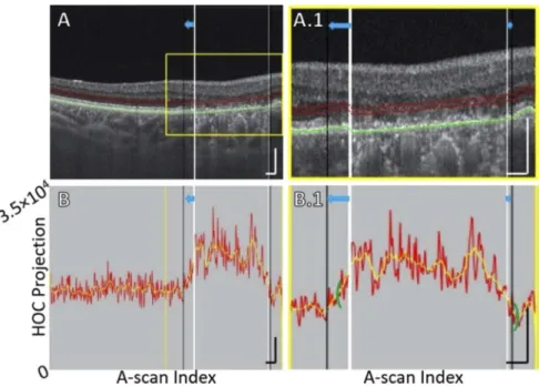
Fig. 1. HOC slab location and boundaries in a pathology-free region of Case 5 (see Table1). (A) OCT B-scan. Red contours correspond to the anterior and posterior boundaries between which the HOC projection was computed. The green contour corresponds to the RPE maximum contour, which was used to generate the HOC projection boundaries. (A.1) Enlargement of panel A. (B) HOC projection values corresponding to panel A are indicated by the red graph (values correspond to a 16-bit OCT B-scan); for ease of interpretation, a smoothed trendline is indicated by the orange graph. (B.1) Enlargement of panel B. All scale bars are 250 µm.

distances were computed as the arclengths of these growth trajectories; and, finally, the local growth rate for each margin position was computed as the trajectory arclength divided by the inter-visit time.

2.8. Statistical analysis

Associations between local HOC projection values and local GA growth rates were assessed using Pearson’s correlation; the null hypothesis was that the Pearson’s correlation between local HOC metric values and local GA growth rates was zero. The level of statistical significance was set at α= 0.05 and to control for the family-wise-error-rate, p-values were compared to the Bonferroni-corrected significance level αBC= α / 7. Because there is substantial (spatial) autocorrelation for both the local HOC and local GA growth metrics, metric values sampled at different margin locations are, in general, not independent, violating the assumptions of standard tests of statistical significance. To address this, we adopted the non-parametric, Monte Carlo approach developed in Viladomat et al., which accounts for spatial autocorrelations [25]. In this approach, for each Monte-Carlo run, the HOC metric values along the margin are randomly permuted and then adjusted so as to have a variogram matching that of the unpermuted values. Using this approach, a null distribution of correlation coefficients can be constructed, which can then be used to compute p-values. For further details, we refer readers to Viladomat et al. [25]. For this study, we performed 10,000 simulation runs for each eye; the variogram smoothing

parameter, h, was set at the empirically determined value of h= 10; in cases in which there were more than 1000 sampled points along the margin, a random sample of 1000 positions was taken.

3. Results

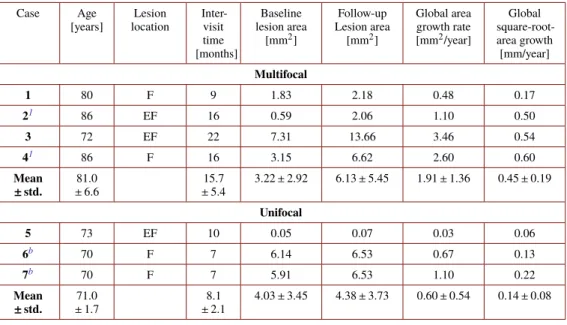
Seven eyes from 5 patients were included in this study. Patients had multifocal as well as unifocal GA lesions and were imaged longitudinally. A summary of patient characteristics is presented in Table1. Qualitative comparisons between local HOC metrics and local GA growth rates are shown in Fig.2and Fig.3. Local HOC metrics and local GA growth rates were calculated and mapped along the baseline GA margin. Variation of the local HOC metric and local GA growth rate can be seen by the colored perimeter on the lesions and qualitative spatial correlation between the HOC metric and GA growth can be seen by comparing the colors. For example, Case 1 in Fig.2shows a low spatial correlation, while Case 4 in Fig.3shows a high spatial correlation. Figure4shows scatter plots of local GA growth versus local HOC metric. Quantitative analysis revealed significant correlations between local HOC metrics and local GA growth rates in 2 of the 7 tested eyes (Case 4 and Case 7; see Fig.4). Although the study cohort is too small to draw conclusions or generalize the HOC results to other patient cohorts, the statistics presented here are intra-eye, and are therefore not a function of the cohort size.

Table 1. Description of Subjects

Case Age [years] Lesion location Inter-visit time [months] Baseline lesion area [mm2] Follow-up Lesion area [mm2] Global area growth rate [mm2/year] Global square-root-area growth [mm/year] Multifocal 1 80 F 9 1.83 2.18 0.48 0.17 21 _{86 EF 16 0.59 2.06 1.10 0.50} 3 72 EF 22 7.31 13.66 3.46 0.54 41 _{86 F 16 3.15 6.62 2.60 0.60} Mean ± std. 81.0 ± 6.6 15.7 ± 5.4 3.22 ± 2.92 6.13 ± 5.45 1.91 ± 1.36 0.45 ± 0.19 Unifocal 5 73 EF 10 0.05 0.07 0.03 0.06 6b _{70 F 7 6.14 6.53 0.67 0.13} 7b _{70 F 7 5.91 6.53 1.10 0.22} Mean ± std. 71.0 ± 1.7 8.1 ± 2.1 4.03 ± 3.45 4.38 ± 3.73 0.60 ± 0.54 0.14 ± 0.08 a_and

Research Article Vol. 11, No. 9 / 1 September 2020 / Biomedical Optics Express 5186

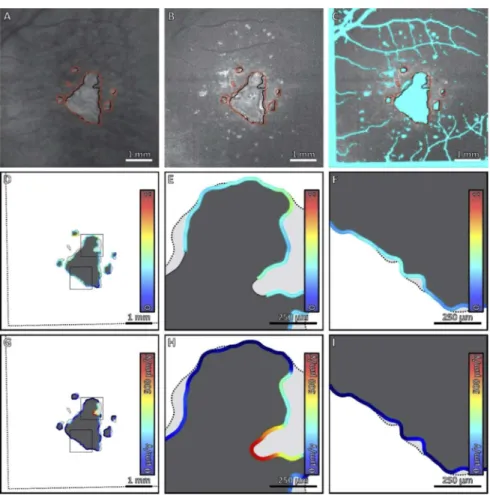
Fig. 2. Comparison of local HOC metric and local GA growth rate along the margin of

GA for Case 1. (A) Sub-RPE OCT projection at baseline; black contours correspond to the lesion margin at baseline, and red contours correspond to the lesion margin at follow-up. (B) HOC projection at baseline. (C) HOC projection, with excluded regions colored teal. (D) Local HOC metric mapped along the baseline GA margin. For visualization, the HOC metric has been normalized between [0,1], with the same normalization used for all cases. (E, F) Enlargements of panel D. (G) Local GA growth rates mapped along the baseline GA margin. (H, I) Enlargements of panel G. Qualitatively, this case has a low spatial correlation between the local HOC metric and the local GA growth.

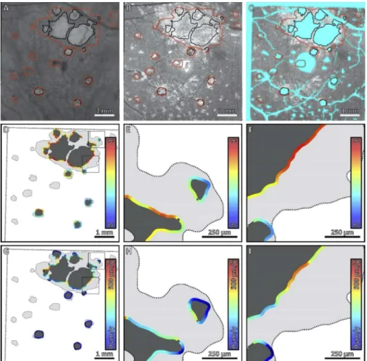
Fig. 3. Comparison of local HOC metric and local GA growth rate along the margin of

GA for Case 4. (A) Sub-RPE OCT projection at baseline; black contours correspond to the lesion margin at baseline, and red contours correspond to the lesion margin at follow-up. (B) HOC projection at baseline. (C) HOC projection, with excluded regions colored teal. (D) Local HOC metric mapped along the baseline GA margin. For visualization, the HOC metric has been normalized between [0,1], with the same normalization used for all cases. (E, F) Enlargements of panel D. (G) Local GA growth rates mapped along the baseline GA margin. (H, I) Enlargements of panel G. Qualitatively, this case has an appreciable spatial correlation between the local HOC metric and the local GA growth rate.

Research Article Vol. 11, No. 9 / 1 September 2020 / Biomedical Optics Express 5188

Fig. 4. Scatter plots of the local GA growth rate versus the local HOC metric values. Local

HOC metric values are normalized between [0,1], with the same normalization used for all cases (as in Figs.2–3). Pearson’s r and the estimated p-values are listed in the top right of each plot. Considering a Bonferroni adjusted significance level, only Case 4 and Case 7 showed statistically significant correlations (asterisks).

4. Discussion

In this study, we proposed the HOC projection as a simple and interpretable OCT-based biomarker of local GA growth. Using a set of quantitative techniques developed in Moult et al. [17], we found a statistically significant correlation between the local HOC metric values along the GA margin and the local GA growth rates in 2 of the 7 tested eyes. This demonstrates the utility of the HOC metric, however, our limited cohort size and heterogeneity of follow-up times preclude making general conclusions.

It is useful to discuss the motivation and rationale for the HOC projection, and to place it in the context of prior OCT and histology studies. The importance of HFL/ONL integrity has been identified by prior studies of GA growth directionality [6,12]. The HOC metric follows a similar strategy to Stetson et al., who proposed OCT minimum intensity as a predictor of GA growth, and found increased minimum intensities predicted where GA grew in 22 of 24 cases [6]. In healthy eyes the minimum intensity along a retinal A-scan occurs in the HFL and ONL. Thus, increased minimum intensities correspond to alterations in these layers. In a study by Niu et al., of 19 retinal features, the thickness of bands from the IPL to EZ and the backscattering of the bands from the OPL to EZ were among the top 5 most predictive of GA growth [12]. Because the HFL and ONL are contained in these ranges, this finding also provides support, albeit indirect, of their importance. Motivated by these findings, and in particular by the approach of Stetson et al., we designed the HOC projection to capture 4 different OCT features of AMD pathology, each of which increases the values of the HOC projection: (1) increased ONL/HFL backscattering; (2) ONL/HFL thinning; (3) descent of retinal layers; and, (4) hyper-reflective foci (HRF). These four OCT features are described below:

1. Increased HFL/ONL backscattering. As reported by Stetson et al., increased OCT minimum intensities, which are located in the HFL and ONL in normal eyes, were associated with areas into which GA lesions grew [6]. Since the HOC slab is comprised of the HFL and ONL, increases in HFL and ONL backscattering also cause increased HOC values.

Although the origin of these backscattering changes is not yet fully understood, Li et al. hypothesized that gliosis may have a role [1]. An example of increased HFL and ONL backscattering along the GA margin is shown in Fig.5.

2. HFL/ONL thinning. AMD is associated with retinal thinning, including thinning of the HFL and ONL. In eyes with GA, Fleckenstein et al. observed severe alterations in every outer retinal band as well as ONL thinning near atrophy borders in most eyes prior to choroidal hyper-reflectivity [26]. In a recent histology study, Li et al. found the distance between the OPL and ELM thinned significantly towards atrophic areas [1]. Among the 170 locations they measured, ONL thickness decreased from ∼30 µm to 0 µm going from regions of non-atrophy to atrophy. The HFL and ONL are hypo-backscattering and their adjacent layers are hyper-backscattering layers. Thus, when the HFL and ONL are thinned, the displacement of adjacent layers into the HOC slab results in an increased HOC signal. An example of HFL and ONL thinning along the GA margin is shown in Fig.6.

3. Descent of retinal layers. In an OCT study by Wu et al. of eyes with drusen-associated atrophy, subsidence of the outer plexiform layer (OPL) and inner nuclear layer (INL) was noted prior to atrophy [27]. Similarly, Bearelly et al. found ONL subsidence was frequently observed beyond the margin of atrophy [28]. And, in a histopathology study, Dolz-Marco et al. defined the GA margin by ELM descent [14]. In the context of our study, subsidence of the retinal layers causes the displacement of the hypo-scattering HFL and ONL out of the HOC slab, and displacement of the relatively hyper-scattering OPL and INL into the HOC slab. Thus, retinal layer descent causes an increased HOC signal. An example of OPL descent into the HOC slab is shown in Fig.7.

4. Hyper-reflective foci. Several groups have reported that hyper-reflective foci (HRF), which are comprised of anteriorly migrating RPE cells, are an indicator of GA progression and development [29–32]. Ouyang et al. [30] suggested HRF as a predictor of new atrophy onset, and, using a deep learning approach, Schmidt-Erfurth et al. [31,32] identified HRF as a predictor of GA progression and development. Since the HOC slab is located anterior to RPE and has a moderate width, it is likely that some anteriorly migrating HRF will be captured by the HOC slab (of course, some HRF may eventually displace beyond the HOC slab). In our cohort, there were no examples of HRF occurring on the GA margins; however, Fig.8shows an example of an HRF—with an “RPE plume” appearance [29]—captured by the HOC slab prior to the formation of a new GA lesion (note also that this HRF occurs within the excluded foveal region). While the HRF of Fig.8did not factor into the results of this study, it nevertheless serves to demonstrate the ability of the HOC slab to capture HRF.

We specified the thickness (∼30 µm) and position (∼80 µm anterior to the RPE) of our HOC slab based on prior ONL and HFL measurements, as well the known variations of the ONL and HFL with eccentricity and age:

1. Spatial variations in ONL and HFL thicknesses. Using directional-OCT, Lujan et al. measured ONL and HFL thicknesses as a function of eccentricity from the fovea, finding a maximum thickness at the central fovea and a rapid decrease parafoveally [24]. Moreover, they reported that ONL thickness is minimum 0.8 mm temporally and 1.0 mm nasally, before gradually increasing up to the periphery of the macula. Based on this spatial thickness variation, and the marked thickness increase at the central fovea, we decided to exclude the central 0.5 mm-radius disk (as discussed in Methods) from our analysis. 2. Macular ONL and HFL thicknesses. Estimated from Fig.3in [24], the average thickness

Research Article Vol. 11, No. 9 / 1 September 2020 / Biomedical Optics Express 5190

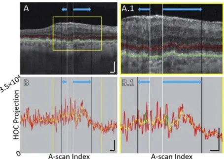
Fig. 5. B-scan analysis of the HOC projection for Case 7, which illustrates increased

ONL/HFL backscattering and other alterations. (A) B-scan. The position of the GA margin at baseline and follow-up are indicated by the white and black vertical lines, respectively (blue arrows indicate growth). Red contours show the anterior and posterior boundaries between which the HOC projection was computed. The RPE maximum contour, shown in green, was used to generate the HOC projection boundaries. (A.1) Enlargement of panel A. (B) HOC projection values corresponding to panel A are indicated by the red graph (from a 16-bit B-scan); for ease of interpretation, a smoothed trendline is shown in orange. (B.1) Enlargement of panel B. The green brackets show the extent of the 125 µm neighborhood over which the HOC metric was computed. All scale bars are 250 µm.

is ∼50 µm. In a histology study by Curcio et al., the mean thickness of OPLHenle (the definition of OPLHenle in [33] is the same layer described in [34,35], which is equivalent to HFL) was reported to be ∼50 µm at 1 mm nasally and ∼55 µm at 1 mm temporally, while the mean thickness of ONL rods was ∼20 µm at 1 mm both nasally and temporally [33]. Note that thickness measured on histologic sections could have shrinkage compared to ex vivo OCT images, leading to an underestimated thickness measurement [33]. Based on these measurements, our ∼30 µm HOC slab should, in normal retinae, cover the majority of the ONL and part of the HFL.

3. Position of the ONL relative to the RPE. Histological measurements by Curcio et al. [33] on a dataset of 18 normal maculae suggest the average distance from the ONL to the mid-RPE is ∼55 µm at 1 mm nasal, and ∼60 µm at 1 mm temporal. However, the thickness measured from ex vivo OCT is larger than histologic sections, with the median area difference between thickness curves being 14.5% (range, 4.0%-39.0%).

4. Changes in HFL and ONL thicknesses and positions with normal aging. In normal aging, Curcio et al. found OPLHenle was 21% thicker in older eyes (≥70 years of age), while ONL thickness did not change significantly with age [33]. They also reported a modest (11%) RPE thinning with normal aging. The thinning of RPE will decrease the distance between the RPE maximum contour and the outer ONL boundary. If the offset distance

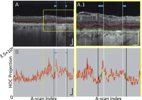
Fig. 6. B-scan analysis of the HOC projection for Case 3, showing ONL/HFL thinning.

(A) B-scan. The GA margin at baseline and follow-up are indicated by white and black vertical lines, respectively (blue arrows indicate growth). Red contours show the anterior and posterior boundaries of the HOC projection. The RPE maximum contour, shown in green, was used to generate the HOC projection boundaries. (A.1) Enlargement of panel A. (B) HOC projection values corresponding to panel A are indicated by the red graph (from a 16-bit B-scan); for ease of interpretation, a smoothed trendline is shown in orange. (B.1) Enlargement of panel B. The green brackets show the extent of the 125 µm neighborhood over which the HOC metric was computed. All scale bars are 250 µm.

(∼80 µm in this dataset) remains fixed, RPE thinning could change the composition of the HOC slab (i.e., include less of the ONL and more of the HFL). However, we expect that the impact on the HOC projection is negligible for the following reasons: (1) RPE thinning is modest (11%); (2) the RPE maximum contour goes nearly through the middle of RPE, which halves the effect of thinning; (3) RPE thinning changes only the ratio of the HFL and ONL in the HOC slab, and both of these layers are hypo-scattering in normal retinae when illuminated with perpendicularly incident beams; and, (4) the HOC projection covers a ∼30 µm slab, which is relatively robust to small offset changes.

The proposed HOC projection has several weaknesses (Table2). First, when the OCT beam is not perpendicular to the retina, the HFL can appear hyper-scattering [34]. Thus, tilted retinae will cause increases in the HOC projection for reasons not related to AMD pathology. One potential approach to mitigate this limitation would be to exclude the HFL from the projection, either by reducing the thickness of the slab, or by directly segmenting the ONL (rather than using an RPE-offset). However, in addition to excluding pathological changes of the HFL, such approaches themselves have limitations: reducing the slab thickness reduces the SNR of the projection, and direct segmentation of the ONL is challenging in non-titled B-scans, where the HFL and ONL can be difficult to distinguish. For these reasons, we recommend the approach of only applying HOC analysis in non-tilted B-scans.

Another limitation of the HOC projection, at least in the form in which it is currently presented, is exclusion of the central foveal region, as well as regions of drusen. In principle, we believe that techniques could be developed to accommodate these regions: for example, spatially-dependent

Research Article Vol. 11, No. 9 / 1 September 2020 / Biomedical Optics Express 5192

Fig. 7. B-scan analysis of the HOC projection for Case 3, showing OPL descent into

boundaries of the HOC projection. (A) B-scan. The GA margin at baseline and follow-up are indicated by the white and black vertical lines, respectively (blue arrows indicate growth). Red contours show the anterior and posterior boundaries of the HOC projection. The RPE maximum contour, shown in green, was used to generate the HOC projection boundaries. (A.1) Enlargement of panel A. (B) HOC projection values corresponding to panel A are shown by the red graph (from a 16-bit OCT B-scan); for ease of interpretation, a smoothed trendline is shown in orange. (B.1) Enlargement of panel B. The green brackets show the 125 µm neighborhood where the HOC metric was computed. All scale bars are 250 µm.

Table 2. Strengths and weaknesses of the HOC projection

Strengths Weaknesses

• The HOC projection is readily interpretable and is underpinned by prior OCT and histopathology studies.

• Based on this pilot study, the HOC projection shows a modest correlation with local GA growth rates in a subset of cases. • The HOC projection is easy to

compute, requiring only Bruch’s membrane and RPE segmentations, which are provided by most commercial OCT systems.

• The HFL can become hyper-scattering in tilted OCT images, thereby confounding analysis.

• Anatomically normal HFL/ONL thickness changes within the fovea require special treatment (in our study, removal).

• Morphological changes in the HFL/ONL layers overlying drusen require special treatment (in our study, removal).

weighting or comparison to normative atlases in the case of the fovea, and direct segmentation, rather than an RPE offset, in the case of drusen. However, this generates additional complexities, and would require larger patient cohorts to develop. Our approach to exclude, rather than accommodate these regions, has the advantage of simplicity, but limits the ability to study these features, both of which are thought to have unique roles in the development and progression of GA. Nevertheless, in the case of the fovea, a separate treatment is likely desirable because of the phenomenon of foveal sparing. Moreover, the importance and role of drusen in the margin-growth of GA remain unclear, with few studies investigating their effects of local GA growth. In a study

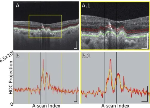
Fig. 8. B-scan analysis of the HOC projection for Case 4, which shows an HRF having an

RPE plume appearance. Note that this RPE plume occurs in the excluded foveal region and corresponds to a new GA focus, rather than an expansion of a previously existing foci; thus, this RPE plume did not factor into our analysis and is instead shown to illustrate the ability of the HOC slab to capture certain HRF. (A) B-scan. There is no baseline GA margin in this B-scan. The position of the GA margin at follow-up is indicated by the black vertical. Red contours show the anterior and posterior boundaries of the HOC projection. The RPE maximum contour, shown in green, was used to generate the HOC projection boundaries. (A.1) Enlargement of panel A. (B) HOC projection values corresponding to panel A are indicated by the red graph (from a 16-bit B-scan; note that, because the hyper-reflective focus generates a high OCT signal, the vertical axis range has been expanded compared to that used Figs.1,5-7); for ease of interpretation, a smoothed trendline is shown in orange. (B.1) Enlargement of panel B. All scale bars are 250 µm.

by Niu et al., when comparing the association of various OCT-derived features in predicting GA growth, the thickness of reticular pseudo-drusen was found to be of high importance, drusen topographic height of mid-range importance, and the binary presence/absence of drusen of low importance [12]. Thus, it is plausible that by excluding drusen the HOC metric reduces its power as a predictive metric.

Beyond the HOC metric itself, our study has several limitations, the most substantial of which is a small cohort size. This, combined with heterogenous follow-up intervals precludes generalization of our findings, and limits our ability to make inferences about why some cases, but not all, showed a spatial correlation between the HOC projection and local GA growth rate. Other limitations include using a single, 1050 nm SS-OCT system, making it difficult to predict if our results will be similar when using other, 840 nm OCT systems.

A general limitation of the HOC metric, common to other image-based metrics, is that the quality of the metric is dependent on the quality of the OCT volume. Consequently, poor quality OCT images (e.g., due to severe refractive errors, media opacities, vignetting) will affect the integrity of the HOC analysis. In this study, eyes with myopia >6 diopters and/or significant media opacities were also excluded, and volumes were assessed for adequate signal-to-noise.

Research Article Vol. 11, No. 9 / 1 September 2020 / Biomedical Optics Express 5194

Reduced OCT data quality will affect all image-based metrics and further analysis is needed to understand whether the HOC metric is more or less sensitive to reduced signal or other artifacts.

5. Conclusion

In this study, we introduce the HOC projection, a simple, physiologically-based OCT metric to assess AMD-related pathology of the outer retina. In a small case series, we spatially correlated the values of the HOC projection along the GA margins with local GA growth rates. The analysis revealed a statistically significant correlation in a subset of cases (2 of 7 eyes). These methods can potentially be used to identify risk markers, stratify patients, or assess response in future therapeutic studies. Future studies with larger patient cohorts are needed.

Funding

China Scholarship Council (201806010297); National Institutes of Health (5-R01-EY011289-31); Topcon Corporation; Retina Research Foundation; Beckman Argyros Award in Vision Research; António Champalimaud Vision Award; Massachusetts Lions Eye Research Fund; Macula Vision Research Foundation.

Acknowledgments

We are grateful to Dr. Rahul Mazumder for fruitful discussions related to assessing the significance of correlations under spatial autocorrelation.

Disclosures

PJR: Apellis (C, I), Biogen (C), Boehringer-Ingelheim (C), Carl Zeiss Meditec (C, F), Chengdu Kanghong Biotech (C), EyePoint (C), Ocunexus Therapeutics (C), Ocudyne (C, I), Unity Biotechnology (C), Valitor (I), Verana Health (I), Stealth BioTherapeutics (F). NKW: Optovue (C), Carl Zeiss Meditec (F), Heidelberg (F), Nidek (F). JGF: Optovue (I, P), Topcon (F).

References

1. M. Li, C. Huisingh, J. Messinger, R. Dolz-Marco, D. Ferrara, K. B. Freund, and C. A. Curcio, “Histology of geographic atrophy secondary to age-related macular degeneration: a multilayer approach,”Retina38(10), 1937–1953 (2018).

2. J. S. Sunness, E. Margalit, D. Srikumaran, C. A. Applegate, Y. Tian, D. Perry, B. S. Hawkins, and N. M. Bressler, “The long-term natural history of geographic atrophy from age-related macular degeneration: enlargement of atrophy and implications for interventional clinical trials,”Ophthalmology114(2), 271–277 (2007).

3. Z. Yehoshua, P. J. Rosenfeld, G. Gregori, W. J. Feuer, M. Falcão, B. J. Lujan, and C. Puliafito, “Progression of geographic atrophy in age-related macular degeneration imaged with spectral domain optical coherence tomography,” Ophthalmology118(4), 679–686 (2011).

4. K. Moussa, J. Y. Lee, S. S. Stinnett, and G. J. Jaffe, “Spectral domain optical coherence tomography–determined morphologic predictors of age-related macular degeneration–associated geographic atrophy progression,”Retina 33(8), 1590–1599 (2013).

5. A. Ebneter, D. Jaggi, M. Abegg, S. Wolf, and M. S. Zinkernagel, “Relationship between presumptive inner nuclear layer thickness and geographic atrophy progression in age-related macular degeneration,”Invest. Ophthalmol. Visual Sci.57(9), OCT299 (2016).

6. P. F. Stetson, Z. Yehoshua, C. A. A. Garcia Filho, R. P. Nunes, G. Gregori, and P. J. Rosenfeld, “OCT minimum intensity as a predictor of geographic atrophy enlargement,”Invest. Ophthalmol. Visual Sci.55(2), 792–800 (2014). 7. R. P. Nunes, G. Gregori, Z. Yehoshua, P. F. Stetson, W. Feuer, A. A. Moshfeghi, and P. J. Rosenfeld, ““Predicting the progression of geographic atrophy in age-related macular degeneration with SD-OCT en face imaging of the outer retina,” Ophthalmic Surgery,”Lasers & Imaging Retina44(4), 344–359 (2013).

8. A. Giocanti-Auregan, R. Tadayoni, F. Fajnkuchen, P. Dourmad, S. Magazzeni, and S. Y. Cohen, “Predictive value of outer retina en face OCT imaging for geographic atrophy progression,”Invest. Ophthalmol. Visual Sci.56(13), 8325–8330 (2015).

9. J. Y. Lee, D. H. Lee, J. Y. Lee, and Y. H. Yoon, “Correlation between subfoveal choroidal thickness and the severity or progression of nonexudative age-related macular degeneration,”Invest. Ophthalmol. Visual Sci.54(12), 7812–7818 (2013).

10. M. Marsiglia, S. Boddu, S. Bearelly, L. Xu, B. E. Breaux Jr, K. B. Freund, L. A. Yannuzzi, and R. T. Smith, “Association between geographic atrophy progression and reticular pseudodrusen in eyes with dry age-related macular degeneration,”Invest. Ophthalmol. Visual Sci.54(12), 7362–7369 (2013).

11. L. Xu, A. M. Blonska, N. M. Pumariega, S. Bearelly, M. A. Sohrab, G. S. Hageman, and R. T. Smith, “Reticular macular disease is associated with multilobular geographic atrophy in age-related macular degeneration,”Retina 33(9), 1850–1862 (2013).

12. S. Niu, L. de Sisternes, Q. Chen, D. L. Rubin, and T. Leng, “Fully automated prediction of geographic atrophy growth using quantitative spectral-domain optical coherence tomography biomarkers,”Ophthalmology123(8), 1737–1750 (2016).

13. M. Lindner, S. Kosanetzky, M. Pfau, J. Nadal, L. A. Gördt, S. Schmitz-Valckenberg, M. Schmid, F. G. Holz, and M. Fleckenstein, “Local progression kinetics of geographic atrophy in age-related macular degeneration are associated with atrophy border morphology,”Invest. Ophthalmol. Visual Sci.59(4), AMD12–AMD18 (2018).

14. R. Dolz-Marco, C. Balaratnasingam, J. D. Messinger, M. Li, D. Ferrara, K. B. Freund, and C. A. Curcio, “The border of macular atrophy in age-related macular degeneration: a clinicopathologic correlation,”Am. J. Ophthalmol.193, 166–177 (2018).

15. M. Thulliez, Q. Zhang, Y. Shi, H. Zhou, Z. Chu, L. de Sisternes, M. K. Durbin, W. Feuer, G. Gregori, R. K. Wang, and P. J. Rosenfeld, “Correlations between choriocapillaris flow deficits around geographic atrophy and enlargement rates based on swept-source OCT imaging,”Ophthalmol. Retina3(6), 478–488 (2019).

16. M. Nassisi, E. Baghdasaryan, E. Borrelli, M. Ip, and S. R. Sadda, “Choriocapillaris flow impairment surrounding geographic atrophy correlates with disease progression,”PLoS One14(2), e0212563 (2019).

17. E. M. Moult, A. Y. Alibhai, B. Lee, Y. Yu, S. Ploner, S. Chen, A. Maier, J. S. Duker, N. K. Waheed, and J. G. Fujimoto, “A framework for multiscale quantitation of relationships between choriocapillaris flow impairment and geographic atrophy growth,”Am. J. Ophthalmol.214, 172 (2020).

18. M. F. Kraus, B. Potsaid, M. A. Mayer, R. Bock, B. Baumann, J. J. Liu, J. Hornegger, and J. G. Fujimoto, “Motion correction in optical coherence tomography volumes on a per A-scan basis using orthogonal scan patterns,”Biomed. Opt. Express3(6), 1182–1199 (2012).

19. S. B. Ploner, J. Schottenhamml, E. Moult, L. Husvogt, A. Y. Alibhai, N. K. Waheed, J. S. Duker, J. G. Fujimoto, and A. K. Maier, “Correction of artifacts from misregistered B-scans in orthogonally scanned and registered OCT angiography,” Invest. Ophthalmol. Visual Sci. 60, 3097 (2019).

20. M. F. Kraus, J. J. Liu, J. Schottenhamml, C.-L. Chen, A. Budai, L. Branchini, T. Ko, H. Ishikawa, G. Wollstein, J. Schuman, J. S. Duker, J. G. Fujimoto, and J. Hornegger, “Quantitative 3D-OCT motion correction with tilt and illumination correction, robust similarity measure and regularization,”Biomed. Opt. Express5(8), 2591–2613 (2014). 21. S. B. Ploner, M. F. Kraus, L. Husvogt, E. Moult, A. Y. Alibhai, J. Schottenhamml, T. Geimer, C. Rebhun, B. Lee, and C. R. Baumal, “3-D OCT motion correction efficiently enhanced with OCT angiography,” Invest. Ophthalmol. Visual Sci. 59, 3922 (2018).

22. Z. M. D. M. H. A. Yehoshua, C. A. A. M. D. Garcia Filho, F. M. M. D. P. Penha, G. P. Gregori, P. F. P. Stetson, W. J. M. S. Feuer, and P. J. M. D. P. Rosenfeld, “Comparison of geographic atrophy measurements from the OCT fundus image and the sub-RPE slab image,”Ophthalmic Surgery, Lasers & Imaging Retina44(2), 127–132 (2013). 23. S. R. Sadda, R. Guymer, F. G. Holz, S. Schmitz-Valckenberg, C. A. Curcio, A. C. Bird, B. A. Blodi, F. Bottoni, U.

Chakravarthy, E. Y. Chew, K. Csaky, R. P. Danis, M. Fleckenstein, K. B. Freund, J. Grunwald, C. B. Hoyng, G. J. Jaffe, S. Liakopoulos, J. M. Monés, D. Pauleikhoff, P. J. Rosenfeld, D. Sarraf, R. F. Spaide, R. Tadayoni, A. Tufail, S. Wolf, and G. Staurenghi, “Consensus Definition for Atrophy Associated with Age-Related Macular Degeneration on OCT: Classification of Atrophy Report 3,”Ophthalmology125(4), 537–548 (2018).

24. B. J. Lujan, A. Roorda, J. A. Croskrey, A. M. Dubis, R. F. Cooper, J.-K. Bayabo, J. L. Duncan, B. J. Antony, and J. Carroll, “Directional optical coherence tomography provides accurate outer nuclear layer and Henle fiber layer measurements,”Retina35(8), 1511–1520 (2015).

25. J. Viladomat, R. Mazumder, A. McInturff, D. J. McCauley, and T. Hastie, “Assessing the significance of global and local correlations under spatial autocorrelation: A nonparametric approach,”Biometrics70(2), 409–418 (2014). 26. M. Fleckenstein, S. Schmitz-Valckenberg, C. Adrion, I. Krämer, N. Eter, H. M. Helb, C. K. Brinkmann, P. C. Issa, U.

Mansmann, and F. G. Holz, “Tracking progression with spectral-domain optical coherence tomography in geographic atrophy caused by age-related macular degeneration,”Invest. Ophthalmol. Visual Sci.51(8), 3846–3852 (2010). 27. Z. Wu, C. D. Luu, L. N. Ayton, J. K. Goh, L. M. Lucci, W. C. Hubbard, J. L. Hageman, G. S. Hageman, and R. H.

Guymer, “Optical coherence tomography-defined changes preceding the development of drusen-associated atrophy in age-related macular degeneration,”Ophthalmology121(12), 2415–2422 (2014).

28. S. Bearelly, F. Y. Chau, A. Koreishi, S. S. Stinnett, J. A. Izatt, and C. A. Toth, “Spectral domain optical coherence tomography imaging of geographic atrophy margins,”Ophthalmology116(9), 1762–1769 (2009).

29. C. A. Curcio, E. C. Zanzottera, T. Ach, C. Balaratnasingam, and K. B. Freund, “Activated retinal pigment epithelium, an optical coherence tomography biomarker for progression in age-related macular degeneration RPE fate in AMD via histology and SDOCT,”Invest. Ophthalmol. Visual Sci.58(1), 211–BIO226 (2017).

30. Y. Ouyang, F. M. Heussen, A. Hariri, P. A. Keane, and S. R. Sadda, “Optical coherence tomography–based observation of the natural history of drusenoid lesion in eyes with dry age-related macular degeneration,”Ophthalmology120(12), 2656–2665 (2013).

Research Article Vol. 11, No. 9 / 1 September 2020 / Biomedical Optics Express 5196

31. U. Schmidt-Erfurth, S. M. Waldstein, C. Grechenig, G. S. Reiter, M. Baratsits, P. Bui, M. Fabianska, M. Arikan, A. Sadeghipour, and H. Bogunovic, “Deep learning identifies hyperreflective foci as predictors of geographic atrophy progression,” Invest. Ophthalmol. Visual Sci. 60, 4222 (2019).

32. U. Schmidt-Erfurth, H. Bogunovic, C. Grechenig, P. Bui, M. Fabianska, S. Waldstein, and G. S. Reiter, “Role of deep learning quantified hyperreflective foci for the prediction of geographic atrophy progression,”Am. J. Ophthalmol.

(2020).

33. C. A. Curcio, J. D. Messinger, K. R. Sloan, A. Mitra, G. McGwin, and R. F. Spaide, “Human chorioretinal layer thicknesses measured in macula-wide, high-resolution histologic sections,”Invest. Ophthalmol. Visual Sci.52(7), 3943–3954 (2011).

34. B. J. Lujan, A. Roorda, R. W. Knighton, and J. Carroll, “Revealing Henle’s fiber layer using spectral domain optical coherence tomography,”Invest. Ophthalmol. Visual Sci.52(3), 1486–1492 (2011).

35. T. Otani, Y. Yamaguchi, and S. Kishi, “Improved visualization of Henle fiber layer by changing the measurement beam angle on optical coherence tomography,”Retina31(3), 497–501 (2011).