WHAT IS NEW WITH THE ACTIVITY WORLD VIEW IN MODELING AND SIMULATION? USING ACTIVITY AS A UNIFYING GUIDE FOR MODELING AND SIMULATION
Alexandre Muzy David R.C. Hill
LISA UMR CNRS 6240 ISIMA/LIMOS – UMR CNRS 6158
Università di Corsica - Pasquale Paoli Clermont-Universite – Blaise Pascal University Campus Grossetti, BP 5220250 Corti, France Campus des Cézeaux – F-63173 AUBIERE Cedex ABSTRACT
Among the four well known conceptual frameworks for simulation, the activity scanning strategy is one possible world-view. Other usual strategies (process-based, event-based or three phase approach) can be used. Depending on the problem to be modeled, one view will be more adapted and ease the implementa-tion. In a system specification, the integration of the usual world-views should be clear. The concept of activity is shared by all the known conceptual frameworks and is a key aspect of simulation. In this paper we emphasize on what is new with activity-based modeling and simulation, and provide new definitions. In addition, we propose a multi-level life cycle adapted to activity aware simulations.
1 INTRODUCTION
The modeling concepts shared in the modeling and simulation community are well known. They include the notions of: systems, models, events, states, variables, entities and attributes, resources, delay and ac-tivities (Law and Kelton 2000; Banks et al. 2000). The concepts of objects and processes have been intro-duced in the simulation community in the late sixties by Dahl and Nygaard (1966) with the Simula lan-guage, though the latter was adopted by the community in the late eighties when object-oriented languages became more widespread and mastered. Around that time Balci (1988) described the four ma-jor frameworks that were in use to implement discrete-event simulation kernels. These conceptual frame-works (also named simulation structures or simulation strategies or world views) guide scientists in the design and the development of their simulation model. In this paper we confer a particular attention to the activity scanning approach and to the activity concept itself.
Activity scanning is also called two-phase approach, the first phase being dedicated to simulation time management, the second phase to the execution of conditional activities (e.g., during scanning, exe-cution of simulation functions depend on the fulfillment of specific conditions). In artificial intelligence this approach is known as rule-based programming (also known as rule-based systems or expert systems) (Chesñevar and Maguitman 2000). Buxton and Laski (1962) introduced this approach in the simulation field with the Control and Simulation Language (CSL). In CSL, when a rule is “fired” a corresponding action is taken and the system state is updated. This approach is often considered to be dual with the event scheduling method. The fourth conceptual framework is named the three phase approach. It is an optimi-zation of the activity scanning approach proposed by Tocher (1963) a year after the introduction of CSL. This optimization is interesting for systems in which potential activities can be detected at each time step. The first phase is the same as in the activity scanning approach. The second phase is different since it handles the execution of all unconditional activities (avoiding rules scanning for rules known to always be fired). The third phase is then similar to the second phase of regular activity scanning (an activity is con-sidered and executed if the corresponding rule can be fired). Pidd (1992) provides more details on the lat-ter approaches. Both activity scanning and three phase approach, as described by the lilat-terature, rely on a fixed time increment. The whole simulation is driven by clock time advance. This time management,
of-ten called clock-based by simulation practitioners, is also named continuous time by theoreticians (Zeigler 1976; Zeigler et al. 2000). Zeigler considers the fixed timed management as a discretization of a continu-ous time function. Because of data structure management, this approach can be inefficient when you get a lot of discrete-event occurrences at the same time, without detecting activities. ). In addition it can also lead to inaccuracies when high precision simulations are considered. An event-based time management where the time is advanced to the next scheduled event avoids the two previously cited problems.
Let’s now consider the theoretical view proposed by Zeigler in 1976, which is a discrete-event speci-fication of the system mathematical structure introduced by Mesarovic (1975). The discrete-event system specification (DEVS) consists of basic elements: discrete-events and models as components composing networks of coupled models (models being atomic or coupled). The trajectory of models in time is driven and executed by abstract simulators. The efficiency of abstract simulators received significant attention (Wainer 2001; Lee and Kim 2003; Hu and Zeigler 2004; Muzy and Nutaro 2005). The execution efficien-cy of simulators depends on their structure (and the basic advantages/disadvantages, which can be ob-tained in distributed and sequential implementation structures), as well as on the structure of the models they are connected to. A choice has to be made between the level of specification of models and the deep-ening of the corresponding simulator hierarchy. We believe that the activity level of a system can be used as a measure of the computational cost of both model and simulator architectures of DEVS. Then, using this measure, a trade-off can be obtained between the reduction of the total execution time and the reusa-bility of the model. This paper provides elements for achieving these goals.
Now that we are placed in a more theoretical context (provided by DEVS), we can review the usual definitions [mainly extracted from (Balci 1988)] of the following words : activity, event, and process, which are the underlying concepts in this paper. An activity is an operation that transforms the state of a system over time. It begins with an event and ends by producing another event (linked to the termination of the activity). Some definitions in the simulation community consider that an activity is thus a period of time with a known duration, constant or random, computed or read in a file if we have a trace based simu-lation. An event is what causes a change in the state of the system (eventually composed of many compo-nents). A process is a sequence of activities or events ordered in time. A process is usually linked to the object, actor or agent oriented approach in which the life cycle of an active entity is specified. As it can be seen, events (underlined in usual definitions) are central for usual world views. We propose here a new fine-grain definition of activity grounded on discrete-events. Then, a full activity-based modeling and simulation life cycle is presented.
The next section of this paper presents the basic operations on DEVS model and simulators and how they can be combined and selected with an activity based approach. This is the first level of the activity-based modeling and simulation. In Section 3, all operations are considered at a core (second level) through the description of the fundamental steps of a simulation life cycle and an abstract framework for decisions, engineering and modeling choices constitutes the last (third level) of the whole approach. Sec-tion 4 presents how the whole life cycle can be applied though a didactical example. Finally, perspectives of this work are provided.
2 ACTIVITY-BASED OPERATIONAL OPTIMIZATION OF MODELS AND SIMULATORS We focus here on the characterization of both modeling and simulation architectures through activity measures. Architectures are evaluated through activity. Switching from one architecture to another is also discussed.
2.1 Usual Operations on Models and Simulator Architectures
Decoupling models and simulators is currently a well accepted conceptual technique in the modeling and simulation community. This allows enhancing reusability and separates modeling and simulation con-cerns improving clarity.
At the model level, the degree of structure specification (or decomposition) of a system (i.e., how much information is known about system internal structure) is related to the degree of autonomy of mod-els:
• First, a fully integrated single model of a system can be considered (this corresponds to a single atomic model). The system is not described by sub-models, just by one model, which consists of a transition function operating on a set of state variables.
• Second, partially autonomous, interdependent, sub-models of the system can be described (this corresponds to a multicomponent model). Usual world views fall in the category of multicompo-nents (Zeigler 2000). Through their transitions, compomulticompo-nents can change directly the state of their influencees.
• Third, fully autonomous modular sub-models of the system can be considered (this corresponds to a coupled model of atomic models). Atomic models interact through input/output ports. Their state is fully encapsulated through port access. Their interface is designed to re-act to input events and to act through output events. In a causal chain, events are sent by influencing components and received by influencees.
At the simulator level, simulators correspond to the computing layer of models. Simulators are in charge of activating transition functions of atomic models, as well as sending events to other models. Co-ordinators are in charge of exchanging messages according to components couplings.
Figure 1 depicts various solutions of model and simulator architecture hierarchies -- for the same sys-tem behavior (i.e., without introducing error). On the left side of the figure, a hierarchy of models is rep-resented (with coupled models CM and atomic models AM). On the right the corresponding fully distrib-uted simulator hierarchy is represented (with coordinators Coo and simulators S). The message exchanges between simulators and managed by coordinators are represented with symbol '*'. Every solution is sup-posed not to affect simulation model trajectories, i.e., to preserve the structure of state variables and the computations performed by the transitions of the model. This hierarchical model and simulator architec-ture, presented as a tree, is coherent with the definitions presented in (Zeigler et al. 2000). However, ar-chitecture changes of models and simulators are considered in a computational way as arar-chitecture opera-tions. Operations are defined and described in detail in the Figure caption. Obviously, a symmetry exists between model and simulator operations: Simulator flattening increases with composition while simulator deepening increases with decomposition. At the last architecture level, a flat simulator is used for simulat-ing the whole modelsimulat-ing hierarchy embedded in coupled model CM3 [more information about the archi-tecture and mechanisms of this kind of simulator can be found in (Muzy and Nutaro 2005).
Moving down or up in the model and/or simulator hierarchy has an execution cost. The less the simu-lation hierarchy is deep (and/or the less the model is decomposed), the faster and the more efficient will be the execution. The more the simulation hierarchy is deep (and/or the more the models are decom-posed), the slower and the less efficient will be the execution.
Moving down or up in the model and/or simulator hierarchy has also a reusability/autonomy cost. When deepening and decomposing, sub-models and sub-simulators are identified as entities, specifying their interfaces. Therefore, because the parts of the simulation models (sub-models and sub-simulators) have well defined interfaces, they can obviously be reused more easily. The less the simulator hierarchy is deep (and/or the less the model is decomposed), the less the models and the simulators can be isolated and reused. The more the simulation hierarchy is deep (and/or the more the model is decomposed), the more the models and the simulators can be isolated and reused.
Figure 1: Various model and simulator architecture solutions. The possible operations are: At the model level: 1. Decomposition: to describe a model with more structure details, moving down through the sys-tem specification hierarchy, using coupled models; and 2. Composition: to reduce the level of specifica-tion of a model, composing submodels into single models, moving up through the system specificaspecifica-tion hierarchy; At the simulator level: 1. Deepening: To add hierarchical levels in order to take into account more detailed operations, and 2. Flattening: To aggregate detailed simulators in a single simulator, thus flattening a hierarchical level.
Before going further, let's precise the notion of autonomy used here. Modular models self-react with their environment (other sub-models) through discrete-event interfaces. If we look at atomic models as rule-based systems, their computations consist of if-then logic re-action elements (the rules) that can be fired (activated) in some causal sequence: If (event of type x received) Then perform computation (or ac-tion). Performing computation possibly leads to a state change. State is then said to be encapsulated. From a control point of view, according to their inputs, atomic models can "decide" to possibly change state or not. This is different from having their state directly changed and accessed, without their authorization, by another component. Therefore, we can say that defining component interfaces increases autonomy. And because autonomy increase leads to adaptability increase (to the external events of component's environ-ment), autonomy increase leads to reusability increase. Notice that the reciprocal is not necessary true.
We end-up here with a new definition of correlated notions of autonomy and reusability in compo-nent-based models:
Definition 0 - Interfaces, autonomy and reusability in component-based models: the Interface of a component consists of its set of input and output ports. Parts (sub-components) of a model are more reus-able and autonomous when described as components interacting through well defined interfaces. If the parts of the model are more reusable, the model itself will be more reusable.
To sum-up, choosing an operation has both advantages and disadvantages in terms of execution time and reusability/autonomy.
2.2 A New Definition of Activity
In usual definitions, activity emerges as a quality of objects. Traditionally, activity, as a measure (a quan-tity), has been scarcely used at the implementation level (Coquillard and Hill 1997), and not at all at the conceptual level (except some recent exceptions we will see). Nonetheless, in all the usual definitions presented in introduction, discrete-events (underlined) are central – as countable units. We propose here a new integrative (qualitative and quantitative) definition of activity.
First, since events occur as a consequence of system activities, we can consider that:
Definition 1 - Qualitative activity in a discrete-event system: A system is qualitatively inactive in case no event occur and qualitatively active in the other case.
Second, at the beginning of the nineties, a C++ simulation library, named Meijin++, proposed an in-teresting implementation of a discrete-event simulation kernel. It proposed a dynamic processing of events with different data structures selecting at runtime the best data structure depending on the number of events, or their frequency of occurrence and on the overhead needed to copy data from one structure to the other. We consider here that:
Definition 2 - Quantitative activity in a discrete-event system: Quantitative activity of a system corre-sponds to the number of discrete-events received by the system, over a simulation time period.
Discrete-events can be of two types: internal or external to the atomic model (endogenous or exogenous).
Definition 3 - Quantitative internal activity in a discrete-event system: Internal quantitative activity corresponds to the number of internal discrete-events, over a simulation time period.
Internal activity provides information about the quantity of internal computations within atomic models. Definition 4 - Quantitative external activity in a discrete-event system: External quantitative activity corresponds to the number of external discrete-events, over a simulation time period.
External activity provides information about the quantity of messages exchanged by atomic models. Definition 5 - Quantitative activity in a discrete-event system: The sum of both internal and external activity is equal to quantitative activity, over a simulation time period.
Quantitative activity measures have been used with success for the simulation of spatially distributed sys-tems in (Muzy et al. 2011). Notice a crucial distinction, quantitative activity is defined at the simulator level and is a metric of computational resource usage, while qualitative activity is defined at the model level although it can be used at the simulator level.
Having proposed a new definition of activity, we want now to know how activity can be used in the usual model and simulator architecture of DEVS. First, considering qualitative activity, atomic models can be defined as embedding a binary state variable: qualitativeActivity={active,inactive}. This has been widely used in DEVS [cf., e.g., (Wainer and Giambiasi 2001; Muzy et al. 2005)], where cells can be ac-tive or inacac-tive]. At each time step, knowing that some atomic models are acac-tive and others are inacac-tive, simulators can focus computations only on active atomic models (Muzy and Nutaro 2005). This is the
ac-tivity tracking mechanism. Hence, acac-tivity tracking is defined as the ability of simulators to automatically detect active atomic models, focusing simulation resources only on these atomic models, during a simula-tion run.
Cellular automata are a good application case for activity tracking. When simulating cellular automa-ta, the Hash-Life algorithm, recently re-introduced in the Golly software (http://golly.sourceforge.net/), is a very good example of activity tracking. Spatial patterns of qualitative activity are detected at various sizes, from the well known elementary patterns to complex meta-cells. A memorization optimization, more classically used in recursive algorithms, uses a hash table, where discovered patterns are directly linked to their simulated future thus avoiding unnecessary re-computation. This activity tracking strategy enables to simulate huge cell spaces (above 1050 cells) on a regular personal computer.
2.3 Level 1: Optimization of Modeling and Simulation Architecture through Activity
As described in section 2.1, a balance exists between the degree of reusability/autonomy and the degree of decomposition/deepening. Therefore, for one simulation model, an optimal satisfying level of depth of model and simulator hierarchy exists. The satisfaction amount depends on a balance between computing resource ratio (computing resource usage over the availability of such resources) and the degree of reusa-bility/autonomy desired. Obviously, when one thinks of infinite computing resources, a modeler would define every sub-model and corresponding simulator at a maximum specification depth. However, this is rarely the case, except for very simple simulation models. The quantification of resource usage is crucial for choosing the adequate depth level of modeling and simulation architecture.
Table 1 presents the model and simulator architecture changes and their impact on reusabil-ity/autonomy, external and internal quantitative activities (noted activities for short). Notice that the im-pact of model/simulator operations on both reusability/autonomy and external activity is symmetric. Composition/flattening decreases external activity but at the same time reusability/autonomy. Decomposi-tion/deepening increases external activity but at the same time reusability/autonomy. Notice too that oper-ations have no impact on internal activity. Therefore, model/simulator operoper-ations have an increasing or decreasing impact on both reusability/autonomy and external discrete-event exchanges.
External activity concerns the definition of sub-models/simulators boundaries. We can say that "the less 'permeable' is this boundary" is a metaphor of how much is isolated an atomic model. In other words, permeability concerns the encapsulation of the state variables of the atomic models. External activity quantifies the degree of encapsulation of atomic models. Therefore, it can be used as a measure of the de-gree of encapsulation in the whole simulation model. Also, as the internal activity measure is equal to a constant, external activity measures here the impact of model/simulator architecture operations on per-formances. Finally, using external activity Table 1 can be considered as a table control of mod-el/simulator architecture operation impacts on encapsulation and performances. Notice that, as described in Figure 1, these operations can be restricted to particular areas of the hierarchy. It is why knowing the negative or positive impact of limited operations is valuable.
Table 1: Level 1 - Activity-based operation balance for modeling and simulation engineering. Sign ‘+’ means an increase and ‘-’ a decrease.
Operation Reuse/Autonomy Internal
Activity External Activity
Model Composition - Unchanged -
Model Decomposition + Unchanged +
Simulator Flattening - Unchanged -
3 ACTIVITY AWARE MODELING AND SIMULATION LIFE CYCLE
Previous section introduced model/simulator architecture changes and how activity can be used to drive architecture change operations in the usual model/simulator hierarchy. Here we go a step further consider-ing models/simulators and their structure changes as a part of modelconsider-ing and simulation life cycle. Struc-ture changes include architecStruc-ture changes and/or structural changes (i.e., a change of simulation model structure). Notice that if a change of architecture does not affect the model behavior, structural changes do.
3.1 Level 2: Definition of the Life Cycle
A life cycle is related to the modeling (and sometimes simulating) tasks. The objects manipulated by the modeler/programmer (models and simulators), and the structure changes on these objects, have been de-fined so far. No confusion should arise between the models/simulators objects, described in the last sec-tion, and the modeling and simulation tasks described here. While models/simulators are objects, the modeling task is the link (set of actions) to build a model of a system. The same way, simulation task is the link (set of actions) to build a simulator of a model.
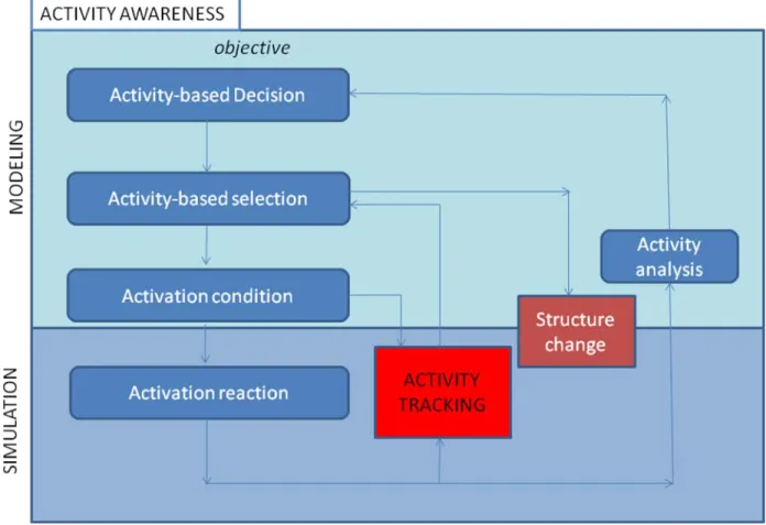
Figure 2 presents how activity can be used as a guide for both modeling and simulation tasks. Figure 2 presents two main parts :
1. The modeling task: and beyond modeling, in the reality this part would correspond to a mind lay-er (and can be refined to decision and modeling processes),
2. The simulation task: and beyond simulation, in the reality this part would correspond to a physi-cal, physiologiphysi-cal, biologiphysi-cal, chemical... layer.
Both parts are consistent with the model/simulator decoupling at the lower level. Simulations will be used as a decision-aid not only for decision makers but for modelers too. At different detail levels, both modelers and decision makers deal with the same objects: decisions, parameters, and resources. Here too, activity can be used to explicitly describe the different steps of modeling and simulation for both decision makers and modelers. This cycle is iterative and structure-variable. Many simulations and structure changes can be iterated. At each iteration, model/simulator structure changes can be achieved. Each step of the cycle deals with activity. This is why the whole cycle is considered to deal explicitly with activity, that is being activity aware. The different steps of the cycle can be described as follows (activity here is quantitative):
1. Objective: An objective can be at three levels: engineering (concerning simulation performanc-es), modeling (concerning model parameters), or decision-support (concerning decisions in the real world);
2. Activity-based decision: Comparing quantitative activity measures from simulation (activity analysis) and the objective, decisions can be achieved.
3. Activity-based selection: According to the decision orders, new model/simulator structures are selected. Information, as sets of active and inactive atomic models, is used from/for the activity tracking module. Activity selection uses these sets for structure changes.
4. Activation conditions: Conditions of activation of atomic models are defined. According to the-se conditions, atomic models become active or not (then composing the active/inactive the-sets for activity tracking).
5. Activation re-actions: If previous condition is fulfilled an activation-related computation can be performed. This computation is considered to be a re-action due to the activation.
6. Activity analysis: A feedback on data activity analysis is obtained in the following ways: Ad-hoc: activity is analyzed from data directly obtained within the simulation loop, or A-priori: activ-ity has been determined from previous analysis and experiments.
Figure 2: Level 2 - Activity aware simulation life cycle. Activity measure is used to perform: Decisions, selection, condition, reaction and analysis.
An activability level can then be determined before the simulation (e.g., a probability function of ac-tivability of a process, of a decision, of a biological behavior, etc.). Activity analysis (Akerkar 2004) of timed data streams consists in determining spatial and temporal activity patterns. As for activity tracking, the detection of activity in data can be based on the causality of events in time and space, for instance, if a particular position in space is active, there is a higher probability that the neighboring positions will turn active.
3.2 Level 3: Definition of the Life Cycle
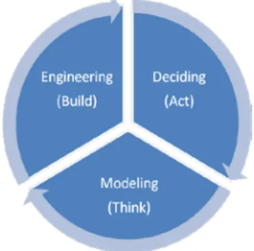
To exploit the activity aware life cycle, we propose a third level of abstraction: the “think-build-act”, process which also consists in interdependent levels (Figure 3) :
1. The Modeling level: following the usual analysis-design-verification-validation cycle, modelers test, evaluate and compare the parameters of the model.
2. Engineering level: the output results obtained at the modeling level are compared to the amount of available resources.
3. Decision-based level: according to the comparison between the obtained results and the availabil-ity of resources, resources can be reallocated. Various scenarios can be used to restrict the initial conditions of the model, having an impact on the allocation of resources. This is the higher level
of the hierarchy. It allows managing solutions through a model base, selecting or not the models according to their performances.
Figure 3: Level 3 - The think-build-act process. This process is iterative and incremental.
The Level 1 - Activity-based operation balance for modeling and simulation engineering, naturally takes place at the engineering level of Level 3 and can be described through the whole Level 2 - Activity aware simulation life cycle (as you will see in the application example hereafter). This process is used on the following application example.
4 AN APPLICATION EXAMPLE: A LAND-USE SIMULATOR
We propose here a didactic simplified version of a land-use simulator (Prunetti et al. 2010). This simula-tor consists of two kinds of stakeholders: the government and landowners. Both can be represented by agent models. The land-use is represented through a cellular model. The following simplified simulation sequence is used. First, the government takes constructability decisions for non built cells. Second, if landowners own the cells concerned by constructability decisions, they choose to protest against this deci-sion or not. Protestation or not of landowners depends on their propensity parameter (being more for con-structability of their cells or not). Third, the government takes a final concon-structability decision according to its own propensity parameter (the government can be more concerned by ecology, the welfare of the landowners or by the fiscal revenues they will obtain if the cells are built).
4.1 Level 3: The Think-build-act Process for Modelers
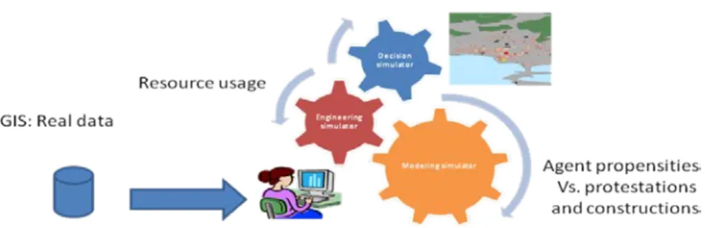
To present a high-level picture of the problem, we present in Figure 4 the Level 3 of our approach -- for modelers. As you will see, the same approach could have been presented for decision-makers and engi-neers, but with different entities. The land-use simulator is composed of three usual simulators, one for each level of our think-build-act process. We assume that each simulator uses real data from a geograph-ical information system. The three simulators have the following roles:
1. The modeling simulator deals with the comparison between output and input parameters: The de-cision making process of landowners and of the government is studied through various input pa-rameter values. Input papa-rameters correspond to the propensity of agents: ecology, welfare and fis-cal revenue (for the government), as well as the constructability desire (for landowners). The impact of every parameter level on outputs (protestations and constructions) is observed to exper-iment the model.
2. The engineering simulator deals with land resources: A resource in this example is linked to the availability of a cell for construction.
3. The decision simulator deals with scenarios: The combination of the model input/output parame-ters constitutes scenarios. A building rate is obtained for every scenario. The modeler will exper-iment various building rates improving his knowledge about the internal structure of the whole
simulation system. If all agents are of the same kind, there are 5 propensity parameters and 6 pos-sible combinations of the parameters (considering, at a time, only 1 government and 3 landowners of each type). If the parameter values are continuous, and if there are many agents, the number of scenarios is exponential.
Figure 4: Simulation process with real data extracted from a Geographical Information System. This is an application of Level 3 for modelers.
4.2 Level 2: Activity Aware Modeling and Simulation Life Cycle for Modelers, Engineers, and Decision-Makers
All the think-build-act process can now be explicitly described through the activity-aware modeling and simulation life cycle. Each step of this cycle (cf. activity rectangles with soft angles in Figure 2) is de-tailed for the three kinds of simulators, representing the behavior of a modeler, an engineer (software en-gineer) and a decision-maker.
4.2.1 Modeler Life Cycle
• Objective: Understand and validate the behavior of the model.
• Activity decision: Quantitative activity = Number of constructions and protestations. Compare: agent parameters (propensity) with output parameters (protestations and constructions). While it is not consistent improve and/or verify the model.
• Activity selection: Activity tracking consists of adding constructions and constructabilities (for active cells) and protestations (from active landowner agents) in space. Structure changes consist in modifying, validating, and verifying the model structure. They exclude architecture changes and related optimizations.
• Activation conditions: They are at the cell level.
- For cells: If (a cell is close to already built cells) Then Consider the cell for construction. - For agents: If (a cell is considered for construction) Then Consider the neighboring
agents for protestation or not. • Activation reactions:
- From government: If (a cell is considered for construction), Then re-act: According to the protestations of the landowners in the neighborhood, make the cell constructible or not. If (the protestations of a cell considered for construction have been collected) Then re-act: Compute the expected fiscal revenue in that cell. If (both protestations and expected cal revenues have been collected for a cell) Then According to the protestations, the fis-cal revenue and the type of the government, the latter makes the cell constructible or not. - For landowners: If (a cell is proposed for construction) Then re-act: protest or not. • Activity analysis: Ad-hoc: Decisions of agents (propositions for constructability and
protesta-tions), A-priori: Activability corresponds to all the probabilities used in the decision making pro-cess, e.g., for protestations.
4.2.2 Engineer Life Cycle
The life cycle for engineers concerns the application of Level 1 - Activity-based operation balance for modeling and simulation engineering.
• Objective: Minimize execution times and maximize reusability through model/simulator archi-tecture.
• Activity decision: Quantitative activity = Number of active atomic models during the simulation, Compare activity and reusability (depth in model/simulator hierarchy). While (execution time is acceptable) Then decompose/deepen the models/simulators. If (execution time is not acceptable) Then look at quantitative activity bottlenecks and compose/flatten the corresponding mod-els/simulators.
• Activity selection: Activity tracking consists of automatically and efficiently select active atomic models, automatically unselect inactive atomic models. This is achieved through an analysis of the activity within the hierarchy through architecture changes. Structure changes of the model are excluded.
• Activation conditions: They are at the atomic model level, which is an abstraction of cells. I.e., for a cell in "consideredForConstruction" state, the corresponding state at the atomic level is "ac-tive". We see here that the state variable for qualitative activity at the atomic level embeds many state variables for qualitative activity at the cell level. Hence, we obtain:
- If (an atomic model receives an event and is in a particular state) Then it becomes active, conversely,
- If (an atomic model does receive an event and is in another a particular state) Then it be-comes inactive.
• Activation re-actions: If (an atomic model is active) Then re-act: compute its transition.
• Activity analysis: Ad-hoc: Number of active atomic models, external and internal evens during the simulation, A-priori: activability corresponds to all atomic models influenced by initially acti-vated atomic models.
4.2.3 Decision-Maker Life Cycle
• Objective: Maximize welfare or/and fiscal revenues to find the best or a set of best scenarios. • Activity decision: Quantitative activity = Protestations (inversely proportional to welfare) of
sce-narios, Minimize protestations and maximize welfare and fiscal revenues.
• Activity selection: Choose the scenarios with a minimum of protestations and a maximum of fis-cal revenues. The decision-maker uses a scenario (or model) base. This allows him to compare scenarios (or models) according to his objectives. Activity tracking consists in keeping scenarios with a minimum of protestations and a maximum of fiscal revenues. This is not a structure change, rather a model (corresponding to scenarios) selection. Architecture changes are excluded too.
• Activation conditions:
- If (a scenario has good performances) Then keep it.
- If (a scenario does not have good performances) Then don't keep it. • Activation re-actions: If (scenario has been kept) Then re-act: evaluate it
• Activity analysis: Ad-hoc: Number of protestations/fiscal revenue of a scenario during the simu-lation. A-priori: All scenarios are tested without a-priori activability.
4.3 Discussion
The whole activity aware multi-level modeling and simulation life cycle proved to integrate: 1. Model/simulator architecture changes,
2. Modeling/simulation steps, and
3. Modeling, engineering and decision levels.
The whole cycle constitutes a new modeling and simulation framework to consider both performance and qualitative results of simulation models, through activity, at many levels (from implementation, to modeling and decision support concerns). Many entities have been specified at many abstraction levels (model/modeling, simulator/simulation, decisions, and engineering). It is, we think, a new perspective aiming at joining optimization and modeling and simulation domains.
5 CONCLUSION
Elements for a discrete-event specification and usual conceptual frameworks for discrete-event simulation have been investigated with a particular attention to the notion of activity. At the simulation level, as a quantitative measure (the number of event occurrences over a simulation time period in the system), and, at the model level, as a qualitative measure (the activation/inactivation of atomic models), activity allows organizing and refining valuable information worth for optimizing: simulation and modeling performanc-es for large simulations, as well as finding an optimal trade-off for the choice of both model and simulator architectures. Furthermore, activity proved to be worth for guiding the modeler through the modeling and simulation life cycle. From a low to a high level of specification, activity allows modeling concisely, and simulating systems efficiently. Moreover, activity can be used to drive the whole modeling and simula-tion cycle. However, a lot of work needs now to be achieved to explore the approach. When many appli-cations will have lead to a knowledge increase about the activity mechanisms and elements, we will con-sider automation tools for activity-based modeling and simulation.
ACKNOWLEDGMENTS
This research is supported by both CNRS and the RTSync Company. We would like to thank deeply Ber-nie Zeigler for his continuous guidance, stimulating discussions, interactive implementations and for providing so much advice concerning the definition of the new activity paradigm, in the name of Science.
We would like also to warmly thank Hans Vangheluwe. Operations on modeling and simulation ar-chitectures emerged from fruitful discussions during research vacations in Corsica.
REFERENCES
Akerkar, S.R. 2004. “Analysis and Visualization of Time-varying data using the concept of 'Activity Modeling”. M.Sc. Thesis. Electrical and Computer Engineering Dept. University of Arizona.
Balci, O. “The implementation of four conceptual frameworks for simulation modeling in high-level lan-guages”. In Proceedings of the 1988 Winter Simulation Conference, 287–295. Piscataway, New Jer-sey: Institute of Electrical and Electronics Engineers, Inc.
Banks, J., J. Carson, B. Nelson, and D. Nicol. 2000. Discrete-Event System Simulation. 3rd ed. Upper
Saddle River, New Jersey: Prentice-Hall, Inc.
Buxton, J. and J. Laski. 1962. “Control and Simulation Language” The Computer Journal, 5:194–199. Chesñevar, C., A. Maguitman and R. Loui. 2000. "Logical models of argument." ACM Comput. Surv., 32 (4): 337-383.
Coquillard, P. and D.R.C. Hill. 1997. Modélisation et Simulation d’Ecosystèmes. Des modèles analy-tiques à la simulation à événements discrets. Collection Ecologie, Masson, Paris.
Dahl, O., and K. Nygaard. 1966. “Simula - An algol based simulation language.” Communication of the ACM, 9:671–678.
Mesarovic M. and Y. Takahara. 1975. General Systems Theory: A Mathematical Foundation. AcademicPress, New York, NY.
Muzy, A. and J. Nutaro. 2005. “Algorithms for efficient implementation of the DEVS and DS-DEVS ab-stract simulators.” In Open International Conference on Modeling and Simulation (OICMS'05), 273– 279.
Pidd, M. 1992. "Object orientation & three phase simulation." In Proceedings of the 1992 Winter Simula-tion Conference, edited by B.L. Nelson, W.D. Kelton, and G.M. Clark, 689–693. Piscataway, New Jersey: Institute of Electrical and Electronics Engineers, Inc.
Hu, X. and B. Zeigler. 2004. “A high performance simulation engine for large-scale cellular DEVS mod-els”. In Proceedings of High Performance Computing Symposium (HPC'04), 6 p.
Law, A. and W. Kelton. 2000. Simulation Modeling & Analysis. 3rd ed. New York: McGraw-Hill, Inc.
Tocher, K.D. 1963. The Art of Simulation, English Universities Press, London.
Lee, W. and Kim T. 2003. “Simulation speedup for DEVS models by composition-based compilation.” In Proceedings of the Summer Computer Simulation Conference, 395–400.
Muzy, A., E. Innocenti, G. Wainer, A. Aiello and J. Santucci, 2005, "Specification of Discrete-event Models for Fire Spreading", Simulation 81(2): 103-117.
Muzy, A., R. Jammalamadaka,B. Zeigler and J. Nutaro. 2010. “The Activity tracking paradigm in dis-crete-event modeling and simulation: The case of spatially continuous distributed systems”, Simula-tion TransacSimula-tions of the Society for Modeling and SimulaSimula-tion InternaSimula-tional, 87(5): 449–464.
Prunetti, D., A. Muzy and E. Innocenti. 2010. "Utilitarian Individual-based Simulation of Real Estate Development in a Computational Virtual Laboratory." Journal of Economic Computation and Economic Cybernetics Studies and Research, 44:159–178.
Wainer, G. and N. Giambiasi. 2001. “Application of the Cell-DEVS paradigm for cell spaces modeling and simulation” Simulation, 76:22–391.
Zeigler, B. 1976. Theory of Modeling and Simulation. John Wiley.
Zeigler, B., H. Praehofer and T. Kim. 2000. Theory of modeling and simulation, 2nd ed. Academic Press.
AUTHOR BIOGRAPHIES
ALEXANDRE MUZY is research fellow CNRS at the Università di Corsica Pasquale Paoli. He received his Ph. D. from the same university, in 2004. He is currently Associate Editor of the SIMULATION Jour-nal (Transactions of The Society for Modeling and Simulation InternatioJour-nal) and member of many con-ference scientific committees. He received in 2011 the Second International Bernard P. Zeigler DEVS Modeling and Simulation award, track Theory and methodology, for his work on activity. His e-mail ad-dress is [email protected].
DAVID R.C. HILL is currently Vice President of Blaise Pascal University (France) since July 2008. Past director of the Auvergne Region Computing Center (CRRI) 2008-2010, he was also deputy director of ISIMA Computer Science & Modeling Institute between 2005-2007. He managed 2 departments at ISIMA between 1995 and 2005. Professor Hill joined ISIMA in 1993, he received his French qualifica-tion as Research Director in 2000 and his Ph.D. in 1993 (dealing with Object-Oriented Software Engi-neering and Simulation) all from Blaise Pascal University. He has served as chairman or program chair-man at various international conferences. He is Associate Editor of the SIMULATION Journal (Transactions of The Society for Modeling and Simulation International), guest editor and reviewer for various simulation and modeling journals. His e-mail address is [email protected].