HAL Id: halshs-00003926
https://halshs.archives-ouvertes.fr/halshs-00003926
Submitted on 4 May 2005
HAL is a multi-disciplinary open access
archive for the deposit and dissemination of
sci-entific research documents, whether they are
pub-lished or not. The documents may come from
L’archive ouverte pluridisciplinaire HAL, est
destinée au dépôt et à la diffusion de documents
scientifiques de niveau recherche, publiés ou non,
émanant des établissements d’enseignement et de
Climate strategy with CO2 capture from the air
David Keith, Minh Ha-Duong, Joshua Stolaroff
To cite this version:
David Keith, Minh Ha-Duong, Joshua Stolaroff. Climate strategy with CO2 capture from the air.
Climatic Change, Springer Verlag, 2006, 74 (1-3), pp.17-45. �10.1007/s10584-005-9026-x�.
�halshs-00003926�
Climate strategy with CO
2
capture from the air
David W. Keith
∗Minh Ha-Duong
Joshuah K. Stolaroff
March 31, 2005
Abstract
It is physically possible to capture CO2directly from the air and immobilize it
in geological structures. Air capture differs from conventional mitigation in three key aspects. First, it removes emissions from any part of the economy with equal ease or difficulty, so its cost provides an absolute cap on the cost of mitigation. Second, it permits reduction in concentrations faster than the natural carbon cycle: the effects of irreversibility are thus partly alleviated. Third, because it is weakly coupled to existing energy infrastructure, air capture may offer stronger economies of scale and smaller adjustment costs than the more conventional mitigation tech-nologies.
We assess the ultimate physical limits on the amount of energy and land re-quired for air capture and describe two systems that might achieve air capture at prices under 200 and 500 $/tC using current technology.
Like geoengineering, air capture limits the cost of a worst-case climate sce-nario. In an optimal sequential decision framework with uncertainty, existence of air capture decreases the need for near-term precautionary abatement. The long-term effect is the opposite; assuming that marginal costs of mitigation de-crease with time while marginal climate change damages inde-crease, then air capture
∗Corresponding author. Department of Chemical and Petroleum Engineering, University of Calgary, 2500 University Drive NW, Calgary, AB, Canada T2N 1N4, [email protected]
increases long-run abatement. Air capture produces an environmental Kuznets curve, in which concentrations are returned to preindustrial levels.
1 Introduction
It is physically possible to capture CO2directly from air and immobilize it in geolog-ical structures. Today, there are no large-scale technologies that achieve air capture at reasonable cost. Yet, several strong arguments suggest that it will be possible to develop practical air capture technologies on the timescales relevant to climate policy [Elliott et al., 2001, Zeman and Lackner, 2004]. Moreover, we argue that air capture has important structural advantages over more conventional mitigation technologies which suggest that, in the long-run, air capture may play a significant role in mitigating CO2emissions.
Air capture may be viewed as a hybrid of two related mitigation technologies. Like carbon sequestration in ecosystems, air capture removes CO2 from the atmosphere, but it is based on large-scale industrial processes rather than on changes in land-use, and it offers the possibility of near-permanent sequestration of carbon. It is also pos-sible to use fossil fuels with minimal atmospheric emissions of CO2by capturing the carbon content of fossil fuels while generating carbon-free energy products, such as electricity and hydrogen, and sequestering the resulting carbon. Like CO2 Capture and Storage (CCS), air capture involves long-term storage of CO2, but unlike CCS air capture removes the CO2directly from the atmosphere and so manipulates the global atmospheric concentration rather than the exhaust stream of large fixed-point sources such as power plants.
This paper hangs on the long-run performance of air capture, a technology that does not now exist at commercial scale. Predicting the performance of technologies a century or more in the future might appear to be a fool’s errand. We embark on it nevertheless because near-term climate policy does depend on long-run estimates of
the cost of mitigating CO2 emissions, whether or not such dependence is considered explicitly.
We don’t believe we can estimate the costs of air capture late in this century with an accuracy of better than perhaps a factor of three. Moreover, we are similarly pessimistic about anyone’s ability to make predictions about any large-scale energy technologies a century in the future. If near-term decisions were strongly contingent on long-run technology forecasts, then the task would be hopeless. As we shall demonstrate in the latter half of the paper, however, the sensitivity of near-term decisions to assumptions about the distant future is sufficiently weak that estimates with this level of uncertainty can provide a meaningful guide to near-term decisions.
We suggest that the two most important factors in estimating the long-run perfor-mance of energy technologies are, first, the basic physical and thermodynamic con-straints and, second, the technology’s near-term performance. Section 2 addresses the first factor, the ultimate physical and economic constraints that may determine the long-run performance of air capture technologies. The second factor is addressed in Section 3, which presents two examples of how air capture might be achieved using current technology. Our view is that air capture could plausibly be achieved at roughly 500 $/tC (dollars per ton carbon) using currently available technologies, and that the com-bination of biomass with CCS could remove carbon from the air at about half that cost. While these technologies are not competitive with near-term mitigation options such as the use of CCS in electric power generation, they may be competitive with other prominent mitigation technologies such as the use of hydrogen fuel-cell cars [Keith and Farrell, 2003].
In the second half of the paper we examine the implications of air capture for the long-run policy and economics of climate change using a global integrated assessment model. The Dynamics of Inertia and Adaptability Model (DIAM) is described in Sec-tion 4. SecSec-tion 5 explores the economic consequences of air capture for global climate policy, by examining how air capture affects optimal CO2emission strategies.
2 Ultimate physical and economic limits on the
perfor-mance of air capture technologies
An air capture system (as we define it) removes CO2from the air and delivers a pure CO2 stream for sequestration. In general, air capture systems will use some sorbent material that selectively captures CO2. The sorbent is then regenerated to yield con-centrated CO2and fresh sorbent ready to be used for capture. A contacting system is necessary to expose the sorbent to fresh air. At the simplest, a pool of sorbent open to the air might serve as a contactor. Active contacting systems might look like water-air heat exchangers that are associated with power plants in which fans blow air past a system of flowing sorbent. Energy is required for regeneration, to pump sorbet and air through the contacting system, and to compress the CO2stream for pipeline transport or sequestration. The energy could be supplied by any source: fossil, solar, or nuclear systems are all plausible.
Extraction of pure gases from air is more than theory: oxygen, nitrogen, and argon are commercially produced by capture from air. The crucial questions about air capture are the cost and energy inputs. In this section we assess some of the ultimate physical limits on the amount of energy and land required to capture CO2from the air. While there are no detailed engineering-economic estimates of performance of air capture technologies, there is a wealth of analysis on the capture of CO2from centralized power plants (although we do not expect that the performance of air capture technologies will approach these limits for many decades). We therefore assess the basic physical and economic factors that influence relationship between the cost of direct CO2 capture from air and the more familiar process of capture from centralized power plants. The relationship between these ultimate limits and nearer term costs is addressed in the following section.
These thermodynamic arguments do not, of course, prove that practical air capture systems can be realized, nor is the performance of air capture technologies likely to
approach thermodynamic limits in the near future. The ultimate thermodynamic limits are nevertheless an important basis for suggesting that air capture can be achieved at comparatively low cost. From the liberation of pure metals from their oxides to the performance of internal combustion engines, electric motors and heat pumps, the historical record strongly supports the view that thermodynamic and other physical limits serve as an important guide to the long run performance of energy technologies.
2.1 Physical limits to the use of energy and land
Thermodynamics provides a lower-bound on the energy required for air capture. The minimum energy needed to extract CO2 from a mixture of gases in which the CO2 has an partial pressure p0 and to deliver it as a pure CO2 stream at final pressure p is set by the enthalpy of mixing, k T ln (p/p0), where k is the Boltzmann constant (8.3 J mol−1K−1) and T is the working temperature. At typical ambient temperatures, k T is about 2.5 kJ/mol. The minimum energy required to capture CO2from the air at a partial pressure of 4 × 10⁻⁴atm and deliver it at one atmosphere is therefore about 20 kJ/mol or 1.6 GJ/tC (gigajoules per ton carbon). If we add the energy required for compressing the CO2to the 100 atm pressure required for geological storage (assuming a 50% efficiency for converting primary energy to compressor work) the overall energy requirement for air capture with geologic sequestration is about 4 GJ/tC.
The ∼4 GJ/tC minimum may be compared to the carbon-specific energy content of fossil fuels: coal, oil, and natural gas have about 40, 50, and 70 GJ/tC respectively. Thus if the energy for air capture is provided by fossil fuels then the amount of carbon captured from the air can—in principle—be much larger than the carbon content of the fuel used to capture it. The fuel carbon can, of course, be captured as part of the process rather than being emitted to the air.
Now consider the requirement for land. Land-use is an important constraint for energy technologies in general, and is a particularly important constraint for biological
methods of manipulating atmospheric carbon that may compete with air capture. An air capture system will be limited by the flux of CO2that is transported to the absorber by atmospheric motions; even a perfect absorber can only remove CO2at the rate at which it is carried to the device by large-scale atmospheric motion and turbulent diffusion. At large scales (100’s of km), CO2transport in the atmospheric boundary layer limits the air capture flux to roughly 400 tC/ha-yr [Elliott et al., 2001].
If air capture is used to offset emissions from fossil fuels as a means to provide energy with zero net CO2 emissions, then we can divide the power provided by the fossil fuels by the land area required to capture the CO2emission resulting from the fuel combustion in order to compute a power density. If coal is used as the fuel, then an air-capture/coal system can provide a CO2-neutral energy flux of 50 W m−2(the value would be almost twice this for an air-capture/natural-gas system).
This result is the effective density at which fossil fuels with air capture provide power with zero net emissions. It may be directly compared with the power densities of alternative CO2-neutral energy systems. Both wind power and biomass based systems can produce roughly 1 W m−2, and even solar power which is constrained much more strongly by cost than by land-use can deliver only ∼20 Wm−2.
There is a strong analogy between the land requirements for air capture and for wind power. Both depend on the rate of turbulent diffusion in the atmospheric boundary layer: diffusion of CO2for air capture and diffusion of momentum for wind power. In each case, large scale processes limit the average flux. Large wind farms, for example, must space their turbines about 5–10 rotor-diameters apart to avoid “wind shadowing” by allowing space for momentum to diffuse downward from the fast moving air above. Similarly for an air capture system, the individual units must be spaced far enough apart to ensure that each receives air with near-ambient CO2-concentration. In each case the footprint of the actual hardware can be limited to only a tiny fraction of the required land because the footprint of an individual wind turbine or air capture system can be small, and the land between the units can be preserved for other uses. If computed
using only the footprints of the individual air capture units, CO2-neutral flux can be many 100’s of W m−2.
The large effective power densities of air capture, however computed, make it im-plausible that land-use could be a significant constraint on the deployment of air cap-ture.
2.2 Capture from the air compared with capture from power plants
Almost all the literature on industrial CO2capture and sequestration has addressed the problem of capturing CO2from large centralized facilities such as electric power plants [Reimer et al., 1999, Willams et al., 2001]. It is therefore instructive to compare the cost of air capture with the cost of capture from these sources.
First, a technical point. One might expect that the energy required to capture CO2 from the air, where its concentration is 0.04% would be much larger than the energy required for capture from combustion streams which have CO2concentrations of 10%. The enthalpy of mixing is logarithmic, however, so the theoretical energy required to capture atmospheric CO2 is only ∼3.4 times the theoretical requirement for capture from a 10% source at atmospheric pressure.
The energy requirement computed from the enthalpy of mixing assumes that the capture system removes only an infinitesimal fraction of the CO2stream (in economist’s terms it’s the value for marginal removals). For real capture systems removing a sig-nificant fraction of the CO2, the energy requirement will be driven by the energy cost integrated up to the last unit of CO2captured. The overall energy requirement increases when the concentration in the discharge air exiting a capture system decreases.
This matters because air capture and power plant capture differ significantly on out-put concentration. The need to make deep reductions in CO2emissions will probably make it desirable to capture most of the CO2from a fossil plant. Indeed most existing design studies have aimed at capturing more the 90% of the CO2in the exhaust gases.
Whereas, in optimizing the overall cost of an air capture system one can freely adjust the faction of CO2which is captured from each unit of air, trading off the energy cost of capture against the cost of moving air through the system. Practical capture systems might capture less than a quarter of the CO2in the air.
Thus it is sensible to compare air capture with CO2removed from a fossil plant at a partial pressure of 10−2(1%) with removal from the air at a partial pressure of 3×10⁻⁴. On these grounds the intrinsic total energy penalty of air capture for delivering CO2at 1 atm is 1.8 rather than the 3.4 derived previously by considering the marginal energy costs of capture1.
Put simply, thermodynamic arguments suggest that capturing CO2from air requires (at minimum) only about twice as much energy as capturing 90% of the CO2from a power plant exhaust. In addition, several economic arguments suggest that the overall difference in costs may well be much smaller because air capture has several practical advantages over CCS.
First, siting issues are less acute for air capture facilities. The location of a CCS power plant is constrained by three transportation requirements: fuel must be trans-ported to the plant, CO2from the plant to a suitable storage site, and finally the carbon-free energy products—electricity or hydrogen—to users. The location of an air capture plant is less constrained: there is no final energy product, and the energy inputs per unit of CO2-output may be as little as 10% (Section 2.1) of that needed for an CCS plant. Moreover, air capture plants will likely be located at CO2 sequestration sites, eliminating the CO2transport cost.
While the cost of transportation is hard to quantify, there is little doubt that reduc-tion in transportareduc-tion requirements lowers the cost of air capture compared to CCS. Perhaps more importantly, it lowers the barriers posed by the siting of new energy
1That is ln(1/10−2)/ ln(1/3× 10−4) = 1.8rather than ln(1/10−1)/ ln(1/4× 10−4) = 3.4. Note that this argument is strictly true only for a one-step capture process.
infrastructure. Public resistance to the construction of new energy transportation in-frastructure such as gas and electric transmission systems is already a serious problem; the development of CCS would only increase these difficulties. It is plausible that the reduction of these barriers is one of the most important attributes of air capture.
Second, air capture systems can be built big, taking maximum advantage of returns-to-scale, because air capture need not be tightly integrated into existing energy infras-tructures. One of the features that makes CCS so appealing is its compatibility with existing fossil energy systems: CO2capture may be though of as a retrofit of the energy system. But this feature also limits the rate of its implementation and the scale of the individual CCS facilities. An power plant with CO2capture may need to be located and sized to replace and existing power plant. Too rapid implementation of CCS will raise adjustment costs. Air capture, in contrast, is more loosely coupled to the existing system: it is not an intermediate but a final energy use. This implies that the air capture facilities can be optimally sized to suit geology and technology, and can be constructed rapidly if required. In this respect air capture is more like geoengineering than it is like conventional mitigation [Keith, 2000].
Finally, air capture differs from CCS because it effectively removes CO2with equal ease or difficulty from all parts of the economy. This is its most important feature. In this section we have argued that the long-run cost of air capture may be quite close to the cost of capture from power plants. But even if the cost of abatement with air capture is considerably more than the cost of abatement at large centralized facilities, air capture still has the unique ability to provide abatement across all economic sectors at fixed marginal cost. Air capture operates on the heterogeneous and diffuse emis-sion sources in the transportation and building sectors where the cost of achieving deep emissions reductions by conventional means are much higher than they are for central-ized facilities.
3 Two examples
We now describe two systems that could demonstrate air capture using existing tech-nology. The first is biomass energy with CCS, and the second is a direct capture system using aqueous sodium hydroxide. We argue that air capture could likely be achieved at costs under 200 $/tC using biomass-CCS or at costs under 500 $/tC with direct air capture.
We say could be achieved because technological developments are driven, in part, by investments in research, development and deployment (RD&D). The development of air capture, or other carbon management technologies, is strongly contingent on the level of RD&D investment. The cost estimates presented below implicitly assume a significant RD&D effort involving the construction of a handful of industrial-scale pilot projects sustained over a couple of decades prior to the large-scale deployment of the technology at a total cost of several billion dollars. We do not assess the likelihood of this assumption, but we do note that similar assumptions underlie many statements about the cost and performance of future energy technologies although they are often unstated.
3.1 Biomass with capture and sequestration
There are many ways in which terrestrial biotic productivity may be harnessed to retard the increase in atmospheric CO2. Biomass may be, (i) sequestered in situ in soil or standing vegetation; (ii) used as an almost CO2-neutral substitute for fossil fuels; (iii) sequestered away from the atmosphere by burial [Metzger and Benford, 2001]; or (iv) used as a substitute for fossil fuels with capture and sequestration of the resulting CO2 [Keith, 2001, Obersteiner et al., 2001]. The latter two options remove carbon from the active biosphere and transfer it to long lived reservoirs.
Biomass with capture provides an energy product—electricity, hydrogen, or ethanol— while simultaneously achieving the capture of CO2from the air. This may allow it to
2 4 6 8 0 50 100 150 200 250 300 Carbon price ($/tC) C os to fe le ct ric ity (c /k W h) Coal Natural gas
Cost of air capture at current electricity prices Biomass with capture
competitive with coal Biomass
with CO capture2
s Figure 1: Cost of electricity as a function of carbon price. The cost and performance of these technologies is uncertain; the robust result is that the cost of electricity from biomass-with-capture declines with carbon price, so that at very high carbon prices it will tend to dominate other options. Similar graphs can be made for the production of hydrogen or ethanol. The following assumptions were used: for natural gas, coal, and biomass with capture, capital costs in $/kW were respectively 500, 1000, and 2000; operating costs were 0.3, 0.8, and 1.0 c/kWhr; efficiencies were, 50%, 40%, and 30% on an HHV basis; and finally, fuel costs were 3.5, 1, and 3 $/GJ respectively. For simplicity, values were adjusted to make the cost of electricity equal for coal and natural gas at a carbon price of zero.
nearly double the effective CO2mitigation in comparison to conventional biomass en-ergy systems. Unlike pure air capture systems, biomass with capture is limited by the availability of biomass. It cannot take advantage of the flexibility that arises from air capture’s decoupling from the energy infrastructure. Nevertheless, biomass with cap-ture provides an important middle ground between conventional mitigation and pure air capture.
Biomass-with-capture systems can be built with existing technology [M’ollerstena et al., 2003, Rhodes and Keith, 2005, Audus, 2004]. Capture is most easily achieved for ethanol production, where a pure CO2stream containing about a third of the carbon in the feedstock is naturally produced from the fermentation step. Existing designs for the production of electricity or hydrogen using biomass gasification technologies can readily be adapted to achieve CO2capture by the addition of water-gas-shift reactors and CO2capture from the syngas stream. While the cost and performance of such tech-nologies is uncertain, all the required component techtech-nologies have been demonstrated commercially.
To derive a carbon price for this technology, consider electricity production. We estimate that a biomass gasification combined cycle power plant with CO2 capture from the syngas using physical absorption in glycol would produce electricity at about 8 c/kWhr while effectively capturing CO2 at a rate of 0.29 kg-C/kWhr [Rhodes and Keith, 2005]. If the electricity were valued at the current producer cost of about 3.5 c/kWhr, then the cost of CO2 capture is about 160 $/tC. If nuclear, wind or CCS technologies set the cost of electricity in a CO2 constrained electric market at 5–7 c/kWhr, then the cost of CO2removal using biomass is about half this value (Figure 1). Unlike fossil-based technologies, the cost of electricity from biomass with capture decreases when the carbon price increases. At a sufficiently high carbon price, biomass with capture becomes relatively cheaper. As can be seen from Figure 1, this occurs well before 160 $/tC. It competes with coal-based electricity (without CCS) at around 100 $/tC.
3.2 Air capture with sodium hydroxide
To illustrate a direct air capture system that could be built with available technology we describe a system based on sodium and calcium oxides that uses technology very closely related to that used in integrated paper mills and the cement industry. We choose this system for ease of analysis and because of its close relationship to cur-rent commercial technologies although we doubt is the best or most likely means of achieving air capture. Put bluntly, our objective is to describe a system most likely to convince skeptics that air capture could be realized with current technologies.
The following description provides an overview of the system; technical details are included in Appendix B. Carbon dioxide is captured in an NaOH solution sprayed through the air in a cooling-tower-like structure, where it absorbs CO2 from air and forms a solution of sodium carbonate (Na2CO3). The Na2CO3is regenerated to NaOH by addition of lime (CaO), forming calcium carbonate (CaCO3). The CaCO3in turn is regenerated to CaO by addition of heat in a process called calcining.
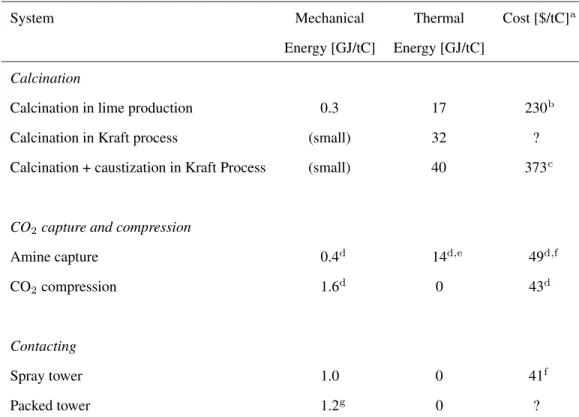
The appeal of this system is that the chemicals involved are all inexpensive, abun-dant, and relatively benign, and that almost all the processes are well-understood as current industrial-scale practices. Given a well-funded R&D program, such a system could be built at large scale within a decade. The energy and monetary costs of the sys-tem are dominated by the calcining portion. This owes to the large amount of chemical energy needed to convert CaCO3to CaO and the energy required to heat and separate the water from the CaCO3 mud entering the caliner. The primary drawback of this system is indeed this large energy requirement.
As a lower bound on the cost of the system, one can consider the current cost of calcining dry CaCO3 without CO2 capture. This is precisely what the lime produc-tion industry does, so we can base this bound on the market price of lime, which gives $240/t-C. To estimate an upper bound, we consider a complete system built from com-ponents from today’s industries. With a minimum of new design, we can assemble
component costs from analogous operations in industry. As described in Appendix B, we find the total cost by this method is roughly $500/t-C.
An optimized system, with a modest amount of new design and novel technology, could be substantially cheaper than $500/t-C, but could not substantially reduce the energy and capital costs of calcining. Still, the NaOH capture scheme is a feasible and scalable near-term option for carbon capture from air.
4 Air capture changes optimal climate policy
The two previous examples suggest that air capture is possible, and that it may be achieved at costs of a few hundred dollars per ton carbon. The cost of air capture is uncertain, but not necessarily much more uncertain than the cost of more conventional emissions abatement technologies half a century in the future. In the remainder of this paper we assume that air capture is available at this cost and explore the consequences for climate policy
It is generally agreed that deep cuts in greenhouse gases emissions will be required to avert dangerous climate change. The debate has often been framed as a problem of defining an appropriate target at which to stabilize atmospheric CO2concentration. This long-term problem can not be solved today, and consequently debates on the op-timal timing for climate policy have failed to converge on a definitive answer to the near-term policy question “how fast should we get there?” [IPCC, 2001, chapters 8.4 and 10.4.3]. Introducing the possibility of air capture casts the discussion in a new light by implying that stabilization is irrelevant, as results presented below will explain.
In this study a stylized integrated assessment model, DIAM, first described by Ha-Duong et al. [1997], is used to compare optimal global CO2 strategy with and with-out air capture. DIAM does not represent explicit individual technologies or capital turnover, but instead the inertia related to induced technical change. The inertia of the worldwide energy system induces adjustment costs, related to the rate of change
0 0.01 0.02 0.03 0.04 0.05 0.06 0.07 0.08 0.09 0.1 300 350 400 450 500 550 600 650 700 750 800
Fraction of world wealth
Atmospheric CO2 concentration (ppmv) Unlucky Lucky Lucky (p=0.8)
Unlucky (p=0.2) Expected impact
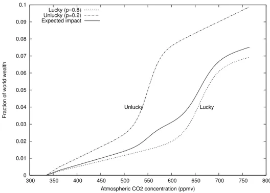
Figure 2: The cost of climate change. The fraction of global wealth lost as a function of carbon dioxide concentration. Damage is assumed to be zero in 2000.
of abatement. The model maximizes the expected discounted inter-temporal sum of utility under the risk of abrupt adverse climate-change impact.
We acknowledge that this cost-benefit optimization framework lacks a special claim to universality, and that it obscures many of the distributional issues that drive climate politics. We adopt it nevertheless, to explore the effect of removing the irreversibility of CO2emissions accumulation via air capture, because of its importance as a reference for considering long-term climate policy.
4.1 Climate change impacts
DIAM represents the uncertainty in the benefits of avoiding climate change, or al-ternatively the cost of climate impact, using one of two non-linear damage functions
represented Figure 2. This frames optimal climate policy as a problem of precaution against a risk of abrupt climate change, as discussed by NAS [2002]. The stochastic impact function represents several defining characteristics of the climate problem: un-certainty regarding climate and ecosystems sensitivity; nonlinearities in the physical and political system; and expected growth in the degree of environmental concern with increasing wealth.
Figure 2’s vertical scale represents a fraction f of global wealth lost. Because of the inertia found in ecosystems and climate system, the impact at date t depends on the lagged concentration, so that (omitting mitigation costs) wealth at date t in the model is W (t) = Wref(t)(1
− f(pCO2(t− 20))). The order of magnitude of the impact
compares with a few years of economic stagnation, since impact costs in the 4–8% range represents a few times the world’s rate of economic growth.
The impact is a function of atmospheric carbon dioxide concentration. While it is measured in monetary units, it represents a global willingness to pay to avoid the given level of climate change, including non-market values. The impact at any date is defined as a fraction of wealth at this date. Therefore it scales over time with the size of the economy. The assumption is that, even though a richer economy is structurally better insulated against climate variations than an poorer economy, the overall desire to limit interference with the biosphere increases linearly with wealth.
Our representation of impacts is consistent with the literature. For example, IPCC [1997, section 3.1.3] reports that for a +2.5 ˚ C warming, economic losses around 1.5 to 2 % of the Gross World Product are commonly used. Because the impacts are expressed as a function of CO2concentrations they implicitly include uncertainty in the climate’s response to radiative forcing as well as uncertainty in climate change impacts.
These uncertainties are summarized as a binary risk in the model. There are two cases, Lucky or Unlucky. If ‘Unlucky’ (p = 0.2) then a 550 ppmv concentration level leads to approximately a 4% impact. If ‘Lucky’ (p = 0.8) then this impact is not re-alized until 650 ppmv. Uncertainty is resolved only in 2040, so that a precautionary
policy has to be found for the period 2000–2040. Expected impact, the weighted aver-age of the two cases, is shown Figure 2 in solid line. Because there is little available evidence to quantify uncertainty further, probabilities are purely subjective.
The impacts are nonlinear; in both cases there is a step in the damage function. As shown in the figure, the main difference is that the step starts at about 600 ppmv in the Lucky case, and 500 ppmv in the Unlucky case.
Rather than imposing a fixed stabilization target, this formulation allows a cost-benefit trade-off. But the kink in the damage function serves as a soft concentration ceiling, and the location of the kink is therefore a critical parameter.
4.2 Abatement cost
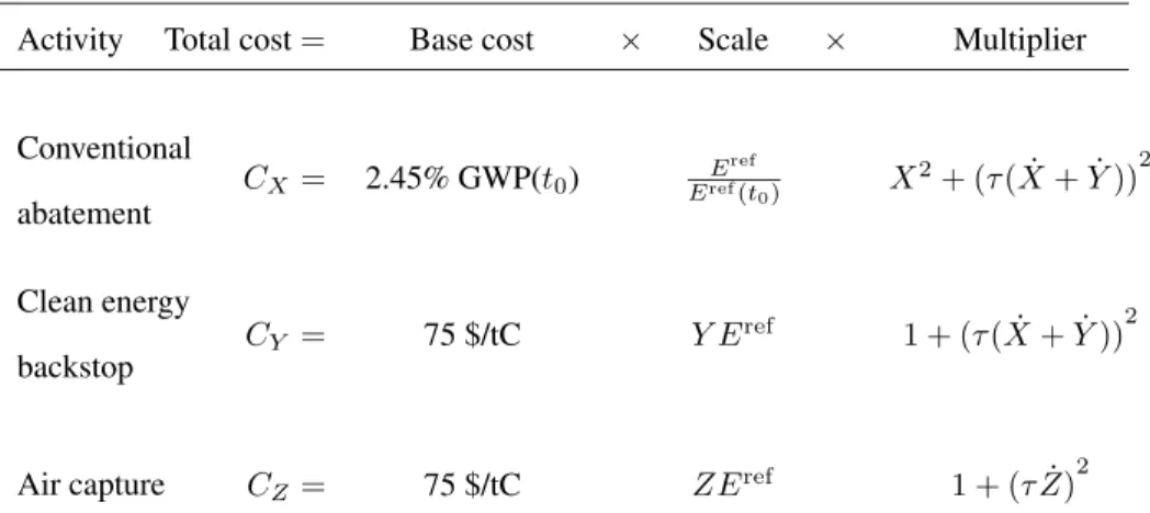
The model represents emissions abatement occurring by three processes, called activi-ties X, Y and Z hereafter, each with its own cost function. Activity X represents emis-sions abatement through conventional existing energy technologies; its marginal cost increases with mitigation. Activity Y represents a conventional backstop technology, for example producing power and hydrogen from solar energy. It reduces emissions at a marginal cost independent of the amount of mitigation. Activity Z represents air cap-ture. The cost of each activity depends on both the scale and rate of its implementation (see Table 1 and Figure 3).
Ignoring adjustment costs, activity X incurs quadratic abatement costs up to full abatement. With adjustment costs, assuming that abatement increases at rate of 2% per year, then the abatement cost function is 4.9X2 per cent of global production. This was calibrated following the DICE-98 model by Nordhaus [2002]. This is represented in Figure 3 by curve X. It says, for example, that if implemented over 50 years, a 100 $ tax per ton of carbon would produce a 40% reduction in emissions.
Activity Y , the conventional backstop, and activity Z, representing carbon capture and sequestration from the air, look alike with constant marginal costs. But there are
two important differences. First, the potential for conventional and backstop abatement is limited to the baseline, so that X + Y ≤ 1, whereas air capture allows negative net emissions, so Z is not bounded above (see Figure 3, curve XYZ).
The second difference has to do with adjustment costs. Using quadratic adjustment costs to represent the dynamics of inertia and adaptability is the distinguishing feature of DIAM. Section 2.2 argued that air capture is less coupled with the energy system than CCS. This is why adjustment costs for Z depend only on ˙Z, while adjustment costs for the other two activities depend on their joint growth rate ˙X + ˙Y.
The scale of adjustment costs in the model is determined by the characteristic time constant for change in the global energy system. We adopt a time constant, τ, of 50 years—roughly in accord with the historical rate of diffusion for new primary fuels [Gr¨ubler et al., 1999]. This leads to the plausible result that on typical optimal trajec-tories, the rate-dependent and -independent terms in the cost function are comparable.
The previous section provided rough engineering estimates of the near-term cost of air capture, and suggested values in the range 200-500 $/tC. These estimates cannot be easily compared with the cost of various mitigation activities in DIAM for three reasons: (1) because of the use of adjustment costs in DIAM, (2) because of the well known incompatibilities between bottom-up engineering estimates and the top-down economic estimates against which DIAM is calibrated [IPCC, 2001], and (3) because, as we will see below, air capture is not used by the model until after the middle of this century and the long-term costs of air capture likely fall between the near-term cost estimates described in Section 3 and the long-run limits described in Section 2.
As a base case we assume that air capture costs 150 $/tC in the model if it is im-plemented over 50 years (the adjustment time constant). This cost is equivalent to the marginal carbon price that would (if implemented over 50 years) produce a 60% reduction in emissions given our baseline abatement cost curve (Activity ’X’, Figure 3). Although the capture cost used in DIAM is less than half that derived from our engineering estimates the values are comparable. This is roughly consistent with our
Activity Total cost = Base cost × Scale × Multiplier Conventional abatement CX = 2.45% GWP(t0) Eref Eref(t0) X2+ (τ ( ˙X + ˙Y )) 2 Clean energy backstop CY = 75 $/tC Y E ref 1 + (τ ( ˙X + ˙Y ))2
Air capture CZ = 75 $/tC ZEref 1 + (τ ˙Z)2 Table 1: The cost of reducing carbon emissions in DIAM for each activity. Gross World Production (GWP) was about 18 × 1012$ for the base year. All base costs decline at an autonomous technical progress rate of 1 per cent per year. The τ = 50 yr inertia parameter in adjustment costs is the characteristic time of the world’s energy system. engineering cost estimates given that (i) air capture is not used for more than half a century, and (ii) its cost lies in the upper 40% of the mitigation supply curve, above the cost of mitigation for many large-scale point sources, but comparable to, or below, cur-rent engineering cost estimates for mitigating dispersed sources such as transportation where costs can exceed 1000 $/tC Keith and Farrell [2003].
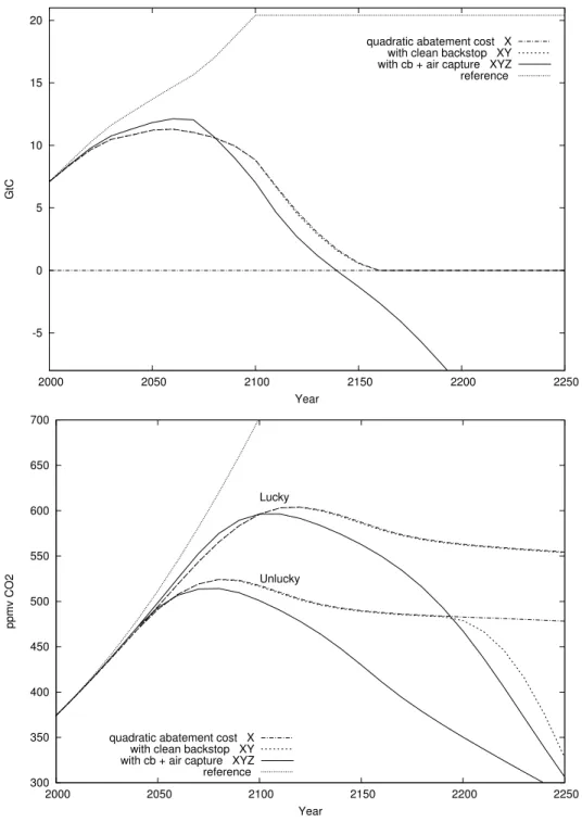
The costs are scaled in time according to the scale of the future energy demand Eref(t), shown in Figure 4, top panel. Reference emissions grow slower than GDP, and then are left constant at 20 GtC/yr after 2100. This baseline is necessarily arbitrary. An important assumption is that the decoupling between GNP and energy consumption observed in industrialized countries after the oil shocks is a persistent general effect.
5 Optimal climate strategies with air capture
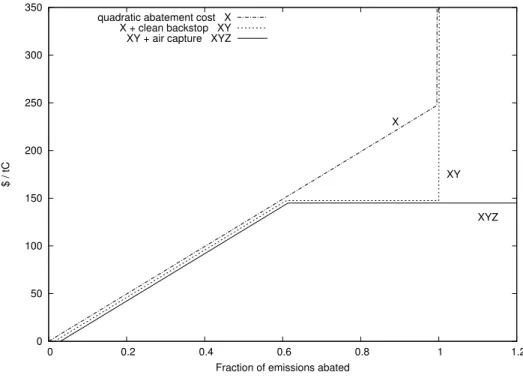
The model was used to compare three scenarios X, XY and XY Z by changing the availability of carbon management activities in the cost function, as Figure 3 illustrates.
0 50 100 150 200 250 300 350 0 0.2 0.4 0.6 0.8 1 1.2 $ / tC
Fraction of emissions abated X
XY
XYZ quadratic abatement cost X
X + clean backstop XY XY + air capture XYZ
Figure 3: Marginal abatement cost functions, assuming that adjustment costs double the long-run permanent costs. Backstop technology allows clean energy without carbon emissions at a constant marginal cost. Air capture allows abatement beyond 100%.
-5 0 5 10 15 20 2000 2050 2100 2150 2200 2250 GtC Year
quadratic abatement cost X with clean backstop XY with cb + air capture XYZ reference 300 350 400 450 500 550 600 650 700 2000 2050 2100 2150 2200 2250 ppmv CO2 Year Unlucky Lucky
quadratic abatement cost X with clean backstop XY with cb + air capture XYZ reference
In scenario X, the backstop Y and air capture Z technologies are not available. Con-sequently, the marginal cost curve is a simple ramp culminating at 250 $ per tC for complete emission abatement. In scenario XY , backstop is available but not direct capture, so that the marginal cost ramp is capped at 150 $ per tC. Finally, scenario XY Zallows all three abatement activities.
Results are displayed Figure 4. The top panel displays the optimal CO2emissions trajectory, where for clarity only the ‘Lucky’ branch (smaller impact) of the contingent strategy is drawn. As acknowledged in previous literature, even in this case emissions have to be deeply reduced in the long run. When air capture is not available, emissions are reduced to zero around 2150. When it is available, air capture kicks-in after 2060 and grows large enough to drive net emissions negative by around 2140.
The first result is that the backstop technology (activity Y ) has almost no effect on the emission trajectory. There are two reasons. First, nonlinearity in the impact function serves as a soft constraint on concentration, as discussed above. The optimum is at the intersection of marginal cost and benefit curves, where the marginal benefit of abatement is steep so the optimal abatement quantity is relatively insensitive to changes in cost.
Another explanation for this result is that the changes in cost are actually relatively small. The carbon value stays below 150 $/tC for a long time, where the backstop makes no difference. Although the backstop’s (Y ) marginal cost is lower than marginal cost of activity X by up to forty percent, this is only relevant in the twenty-second century when the overall costs are a small fraction of global wealth.
The results are similarly insensitive to the cost of air capture. Even if the cost of air capture is doubled to 300 $/tC (including the 50-year adjustment cost), the optimal concentration trajectories are qualitatively similar to those shown here (Appendix A).
The second result is that the concentration overshoots its final level in all cases (Figure 4, bottom panel). Given that the model assumes constant economic growth,
this can be called an environmental Kuznets curve. Most published scenarios have concentrations and climate change increasing monotonically. Even in intervention sce-narios, concentration generally increases asymptotically to a stabilization ceiling. Yet the idea that managed atmospheric pollutants first increase and then decrease with time has been heavily discussed in the environmental economics literature; see, for example, Anderson and Cavendish [2001] or the survey by Borghesi [1999].
Carbon dioxide is a long-lived stock pollutant. Technical progress, the decreasing energy intensity of the economy and the effect of adjustment costs make it comparably cheaper to reduce emissions in the future. These factors explain why the optimal tra-jectory overshoots. Also, an inverted Malthus effect is at play. On one hand, climate change impact is a fraction of wealth. Therefore the willingness to pay to solve the problem grows exponentially. On the other hand, the costs of abatement are propor-tional to the amounts of pollution generated in the business-as-usual scenario, where reference emissions are assumed to grow only up to 2100 and linearly.
The third result elaborates on the previous one: When air capture is available con-centration declines rapidly toward preindustrial levels. Without air capture the dynam-ics that dictate a return toward a low concentration target remain as described above, but the rate of CO2 concentration decline is determined by natural removal. With air capture, the rate is determined by the trade-off between its costs and the benefits of reducing climate change.
This idea is overlooked in the existing literature. Admittedly, the decrease is mostly happening in the twenty-second century, while most scenario studies reasonably focus on this one. Yet the factors driving the return toward preindustrial concentration— the inverted Malthus effect—are general, as is the environmental Kuznets curve. This result suggest that if technology exists to reverse climate damage it will be employed.
The rate at which concentrations return to pre-industrial levels depends on the cost of air capture, but for reasons mentioned in our discussion of the first result above, the
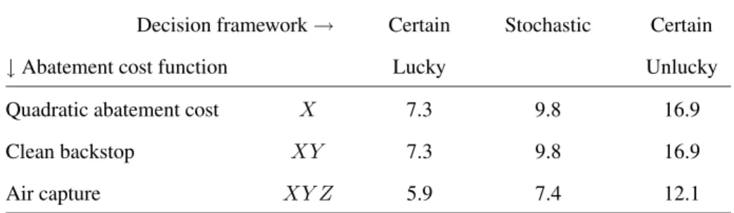
Optimal % abatement in 2030 Decision framework → Certain Stochastic Certain ↓ Abatement cost function Lucky Unlucky Quadratic abatement cost X 7.3 9.8 16.9 Clean backstop XY 7.3 9.8 16.9 Air capture XY Z 5.9 7.4 12.1 Table 2: Abatement (%) of global CO2emissions, in 2030, for the three different abate-ment cost function X, XY and XY Z defined Figure 3. The first column shows the optimal abatement if one were certain from the start that climate impact is low. Con-versely, the third column shows optimal abatement if one knew that climate impact on Figure 2’s higher curve. Central column shows the optimal abatement on a precaution-ary path in a stochastic world, as displayed on Figure 4.
rate is only weakly dependent on cost. The ultimate return to pre-industrial concentra-tions and the rate of return also depend on the role of adaptation in reducing, or pos-sibly eliminating, climate impacts over the long run. We speculate that, if reasonable estimates of long-run adaption were included in the model’s climate-damage function we would still see a prominent concentration peak and subsequent decline (i.e., the Kuznets curve) but that the decline would be slower and, depending on assumptions about adaptation, the concentrations might not return to pre-industrial levels.
The fourth result highlights a short-term implication of air capture. The model com-putes an optimal contingent strategy, given that uncertainty is resolved in 2040. Table 2 shows the optimal emission abatement in 2030 under various uncertainty (columns) and technology availability (rows) scenarios.
The optimal contingent strategy is in the middle ‘Stochastic’ column. The left col-umn, ‘Lucky’ applies when it is known from the start that damages are relatively low. As can be seen, precaution is a middle-of-the road approach, leaning on the optimist
side towards the ‘Lucky’ outcome, which is expected (p = 0.8).
Air capture reduces initial abatement. Abatement is 9.8 percent below business as usual in the X case, but only 7.4 percent with air capture XY Z (Table 2). Because the total costs are initially quadratic, this difference in abatement corresponds to a much larger difference in spending on abatement: $13 billion per year with air capture, and $24 billion without. This effect arises even though air capture is not until long after 2030 and is due to the possibility of moderating future impacts in the ‘Unlucky’ case.
The result can be understood as the reduction of the environmental irreversibility: it is optimal to pollute more when it is possible to cleanup afterward than when it is not.
This fourth result suggests that air capture reduces an important irreversibility from the decision problem. Note however that the irreversibility in impacts themselves was not modeled. This aspect does have significant policy implications, as we discuss next. While air capture may reduce our vulnerability to extreme climate responses, it does not necessarily allow us to eliminate consequences. The time-scale for abrupt climate change may be as short as a few decades. If an abrupt change occurred— suppose a rapid shutdown of the thermohaline circulation—a large scale air capture program might conceivably be built in a comparable time frame, but it would need to operate continuously for several decades to significantly decrease the atmospheric concentration of CO2. Air capture is therefore unable to eliminate vulnerability to such rapid changes.
More generally, air capture eliminates only the irreversibility of atmospheric carbon dioxide accumulation in the long run. It does not address irreversibilities in climate change damages. This distinction is critical because of many remaining unknown time constants in the links between CO2concentration, global warming, earth climate, and human activities. Further research is needed to model explicitly abrupt climate damage with hysteresis.
6 Conclusion
No air capture systems exist today, yet we argued that one could be readily built with-out any new technology, and that in the long run, the ability to capture CO2 from the air fundamentally alters the dynamics of climate policy (even if it is more expen-sive than any conventional mitigation available in the economy). Air capture differs from conventional mitigation in three key aspects. First, it removes emissions from any part of the economy with equal ease or difficulty. Consequently, its price caps the cost of mitigation with a scope unmatched by any other kind of abatement technology. Second, because air capture allows the removal of CO2after emission it permits reduc-tion in concentrareduc-tions more quickly than can be achieved by the natural carbon cycle. Third, because it is weakly coupled to the energy system, air capture may offer stronger returns-to-scale and lower adjustment costs than conventional mitigation options.
This is not to claim that air capture systems are trivial to build today, nor that they will play a quantitative role in the next decade. With regard to the technology, we advanced three arguments. First, that both thermodynamics and economic reasons sug-gest that in the long run, the cost of large-scale air capture will be roughly comparable to the cost of capturing CO2from large fixed sources. Second, we have described two systems that could plausibly achieve air capture a costs from 200 to 500 $/tC within the next few decades. Finally, while their costs are large compared to near term carbon prices, they are competitive with, or significantly cheaper than, the cost of abatement from diffuse sources found in the transportation sector. While both costs will likely decline with technological improvement, air capture is likely to be competitive with conventional mitigation when the time comes to achieve very deep reductions in emis-sions.
Several research groups [McFarland et al., 2004, Herzog et al., 2003, Keller et al., 2003, for example], have begun to explore the implications of carbon management technologies and the leakage of sequestered carbon using integrated assessment
mod-els. Our paper extends this work by exploring the role of direct air capture.
The most obvious impact of carbon management technologies is in altering the cost of mitigation. The model used here, DIAM, is designed to explore climate policy over century-long time-scales and contains a very simplistic representations of the energy sector. From such a perspective, including CCS is achieved by a rather minor adjust-ment to the aggregate abateadjust-ment cost function. Consequently, while mitigation using CCS may differ in many important dimensions from mitigation achieved using non-fossil renewables, the outcomes in terms of cost-benefit optimal emission strategy was very similar.
Absent air capture or the possibility of unlimited biological sequestration, leak-age of sequestered carbon presents novel problems with respect to the inter-temporal distribution of abatement costs and benefits. If industrial carbon management plays a dominant role in mitigating emissions, then as much as 500 GtC could be stored by 2100. Even if the average leak rate is only 0.2 percent annually, there would be a 1 GtC per year source undermining CO2stabilization. As [Keller et al., 2003, Figure 4] has shown, absent air capture the leakage issue has significant consequences on optimal long-term climate policy.
This problem may be compounded by the CCS energy cost, which is likely to result in somewhat faster mobilization of the fossil carbon reserves than in a business-as-usual scenario: the 500 Gt of fossil carbon would be burned sooner with CCS than without.
Air capture, or any similar means of engineering a near-permanent carbon sink, reduces the leakage problem to a relatively minor perturbation in the distribution of abatement cost over time.
Previous research suggested that when carbon dioxide accumulation is irreversible, the ultimate concentration target is the most important parameter for the timing of abatement. For example, if it is assumed that CO2concentration will be stabilized at 600 ppmv or over, then there is little cause for action before 2020. The opposite holds if
the ultimate ceiling is 450 ppmv, or if one wishes to keep open the option of remaining below that ceiling.
But this stock irreversibility is less relevant when capture from the air is possi-ble. Our simulations demonstrate that air capture can fundamentally alter the temporal dynamics of global warming mitigation.
Air capture is a form of geoengineering because it directly modifies the biosphere and would be implemented with the aim of counterbalancing other human actions [Keith, 2000]. Like geoengineering, its availability reduces our vulnerability to some high-consequence low-probability events. In an optimal sequential decision frame-work, we have shown that the consequence is a decrease in the need for precautionary short-term abatement. Because air capture may provide some insurance against cli-mate damages, it presents a risk for public policy: the mere expectation that air capture or similar technologies can be achieved reduces the incentive to invest in mitigation. Yet, while air capture removes irreversibility in CO2concentration increase, it does not protects against irreversibilities in the climate system’s response to forcing.
While air capture may reduce the amount of mitigation in the short run, it can in-crease it on longer time-scales. If air capture is possible, even at comparatively high cost, and if the willingness to pay for climate change mitigation grows with the econ-omy, then the optimal trajectory follows an environmental Kuznets curve. At some point the optimal target will be to return atmospheric greenhouse gases concentration to lower levels. These may be even lower than present-day levels. Air capture changes the temporal dynamics of mitigation by making this response possible.
Acknowledgments
Research supported by the Centre National de la Recherche Scientifique, France and by the Center for Integrated Assessment of Human Dimensions of Global Change, Pitts-burgh PA. This Center has been created through a cooperative agreement between the
National Science Foundation (SBR-9521914) and Carnegie Mellon University, and has been generously supported by additional grants from the Electric Power Research In-stitute, the ExxonMobil Corporation, and the American Petroleum Institute. We thank Hadi Dowlatabadi, Granger Morgan, Ted Parson, Hans Ziock, Klaus Keller and Alex Farell for their useful comments.
References
Dennis Anderson and William Cavendish. Dynamic simulation and environmental policy analysis: Beyond comparative statistics and the environmental Kuznets curve.
Oxford Economic Papers, 53(4):721–746, October 2001.
Harry Audus. Climate change mitigation by biomass gasification combined with CO2 capture and storage. In Proceedings of 7th International Conference on Greenhouse
Gas Control Technologies, volume Volume 1: Peer-Reviewed Papers and Plenary
Presentations, Cheltenham, UK, 2004. IEA Greenhouse Gas Programme.
Simone Borghesi. The environmental Kuznets curve: a survey of the literature. Tech-nical Report Nota do lavoro 85.99, Fondazione Eni Enrico Mattei, November 1999. URL http://www.feem.it/web/resun/wp/85-99.html.
S. Elliott, K. S. Lackner, H. J. Ziock, M. K. Dubey, H. P. Hanson, S. Barr, N. A. Ciszkowski, and D. R. Blake. Compensation of atmospheric CO2buildup through engineered chemical sinkage. Geophysical Research Letters, 28(7):1235–1238, 2001.
Peter Flanagan. Email conversation. Associated with Groupe Laperrire and Verreault, May 2004.
by scrubbing with caustic soda in packed towers. Transactions of the Institution of
Chemical Engineers, 31:201–207, 1953.
Arnulf Gr¨ubler, Nebojˇsa Naki´cenovi´c, and David G. Victor. Dynamics of energy tech-nology and global change. Energy Policy, 27:247–280, 1999.
Minh Ha-Duong, Michael J. Grubb, and Jean-Charles Hourcade. Influ-ence of socioeconomic inertia and uncertainty on optimal CO2-emission abatement. Nature, 390:270–274, 1997. URL file://HaDuong. ea-1997-InfluenceInertiaUncertaintyAbatement.pdf.
H. Herzog, K. Caldeira, and J. Reilly. An issue of permanence: Assessing the effec-tiveness of temporary carbon storage. Climatic Change, 59, 2003.
P.J. Hoftyzer and D.W. van Krevelen. Applicability of the results of small-scale exper-iments to the design of technical apparatus for gas absorption. Transactions of the
Institution of Chemical Engineers, Supplement (Proceedings of the Symposium on Gas Absorption, 32:S60–S67, 1954.
IPCC. Stabilisation of Atmospheric Greenhouse Gases: Physical, Biological and
Socio-economic Implications (IPCC Technical paper III). UNEP/WMO, 1997.
Working Group I.
IPCC. Climate Change 2001: Mitigation. Cambridge University Press, 2001.
N.A.C. Johnston, D.R. Blake, F.S. Rowland, S. Elliott, K.S. Lackner, H.J. Ziock, M.K. Dubey, H.P. Hanson, and S. Barr. Chemical transport modeling of potential atmo-spheric CO2sinks. Energy Conversion and Management, 44(5):683–691, 2003. David W. Keith. Geoengineering the climate: History and prospect. Annual Review of
Energy and the Environment, 25:245–84, 2000.
David W. Keith. Sinks, energy crops, and land use: Coherent climate policy demands an integrated analysis of biomass. Climatic Change, 49:1–10, 2001.
David W. Keith and Alexander E. Farrell. Rethinking hydrogen cars. Science, pages 315–316, 2003.
Klaus Keller, Zili Yang, and Matt Hall. Carbon dioxide sequestration: When and how much? Working Paper Series 84, Princeton University, Center for Economic Policy Studies, 2003. In revision for Climate Change.
J.R. McFarland, J.M. Reilly, and H.J. Herzog. Representing energy technologies in top-down economic models using bottom-up information. Energy Economics, 26: 685–707, 2004.
R. A. Metzger and G. Benford. Sequestering of atmospheric carbon through permanent disposal of crop residue. Climatic Change, 49:11–19, 2001.
Kenneth M’ollerstena, Jinyue Yana, and Jose R. Moreirab. Potential market niches for biomass energy with CO2capture and storage—opportunities for energy supply with negative CO2emissions. Biomass and Bioenergy, 25:273–285, 2003.
National Academy of Science NAS. Abrupt climate change: inevitable surprises. Na-tional Academy Press, Washington, D.C., 2002. ISBN 0-309-07434-7.
William D. Nordhaus. Modeling induced innovation in climate-change policy. In Ar-nulf Gr¨ubler, Nebojsa nakicenovic, and William D. Nordhaus, editors, Technological
change and the environment, chapter 8, pages 182–209. Resources For the Future,
2002.
M. Obersteiner, C. Azar, P. Kauppi, K. M¨ollersten, J. Moreira, S. Nilsson, P. Read, K. Riahi, B. Schlamadinger, Y. Yamagata, J. Yan, and J.-P. van Ypersele. Managing climate risk. Science, 294(5543):786–787, October26 2001.
Anand B. Rao and E. S. Rubin. A technical, economic, and environmental assessment of amine-based CO2 capture technology for power plant greenhouse gas control.
Environmental Science and Technology, 36(20):4467–4475, 2002.
P. Reimer, B. Eliassed, et al., editors. Greenhouse gas control technologies:
Proceed-ings of the 4th international conference, Interlaken, Switzerland, 1999. Pergamon.
J. S. Rhodes and D. W. Keith. Engineering-economic analysis of biomass IGCC with carbon capture and storage. Biomass and Bioenergy, (submitted), 2005.
J. K. Stolaroff, G. V. Lowry, and D. W. Keith. Using CaO- and MgO-rich industrial waste streams for carbon sequestration. Energy Conversion and Management, 46 (5):687–699, 2005.
Robert C. Weast, editor. CRC Handbook of Chemistry and Physics. CRC Press, Boca Raton, FL, 2003.
D. Willams, B. Durie, P. McMullan, C. Paulson, and A. Smith, editors. Greenhouse gas
control technologies: Proceedings of the 5th international conference on greenhouse gas control technologies, Collingwood, Australia, 2001. CSIRO Publishing.
Frank S. Zeman and Klaus S. Lackner. Capturing carbon dioxide directly from the atmosphere. World Resources Review, 16:62–68, 2004.
A Sensitivity analysis
Abatement 2030 Maximum Year 2200 fraction BAU ppmv CO2 ppmv CO2
L or U L U L U X = Quadratic abatement cost 0.10 604 524 563 482 XY = X+ Clean backstop 0.10 603 524 562 478 XYZ = XY+ Air capture 0.07 596 514 467 350 D = XYZ+ Air capture 300$/tC 0.09 604 521 518 410 E = XYZ+ No lag in damage 0.09 583 506 401 337 F = XYZ+ Better lucky case 0.06 678 515 527 349 GX = X+ Bad surprise close 0.10 603 505 562 437 GXYZ= XYZ+ Bad surprise close 0.07 596 485 470 337 I = XYZ+ Air capture ≤ 2GtC yr−1 0.09 600 520 538 443 Optimal strategies are characterized by five key numbers. First, the optimal percentage of global CO2emissions abatement in 2030 shows how much precaution is incorpo-rated in the strategy, before uncertainty resolution. The second and third characteristics are the magnitude of the atmospheric CO2concentration peak, in ppmv, for the Lucky, ‘L’, and Unlucky, ‘U’ states of the world. Columns four and five display the maximum concentration and concentration in 2200, respectively, for the U and L states.
Runs X, XY and XYZ explore different cost abatement functions as discussed in the body of the text. Runs D and F each use the XYZ damage function, but Run D doubles the cost of air capture while Run E removes the lag in the damage function. Run F has abrupt climate damage in the ‘Lucky’ case kicking in at 705 ppmv instead of 605.
Conversely, runs GX and GXYZ have abrupt climate damage in the ‘Unlucky’ case kicking in at 450 ppmv instead of 511, with a probability 5 percent instead of 20. Finally, in Run I the use of air capture is restricted to 2 GtC/yr, to explore the role of
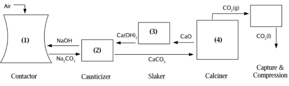
Figure 5: Top level process diagram of an example direct air capture system. Closed chemical loops of NaOH and CaO extract CO2from air convert it to a pure, compressed form for sequestration.
biomass capture alone under the assumption that biomass supply would be limited. Runs GX and GXYZ combine this damage with the cost function from run X and run XYZ, respectively. They represent the risk of early abrupt climate damage without capture.
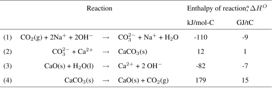
Table B.1: Chemistry of Na/Ca capture system
Reaction Enthalpy of reactiona, ∆HO kJ/mol-C GJ/tC (1) CO2(g) + 2Na++ 2OH− → CO2−
3 + Na++ H2O -110 -9 (2) CO2−
3 + Ca2+ → CaCO3(s) 12 1 (3) CaO(s) + H2O(l) → Ca2++ 2 OH− -82 -7 (4) CaCO3(s) → CaO(s) + CO2(g) 179 15 a Derived from Weast [2003].
B Example direct air capture scheme
B.1 Overview
The example system proposed here uses an aqueous solution of sodium hydroxide (NaOH) to capture CO2 from the air and then regenerates this solution. A top-level process diagram was presented in Figure B.1. The chemistry of the system is summa-rized by the reactions in Table B.1.
In the Contactor, the NaOH is brought into contact with atmospheric air and ab-sorbs CO2, forming sodium carbonate (Na2CO3). This carbonate-containing solution is then sent to the Causticizer. In the Causticizer, lime (CaO) is added to the solution, producing solid calcium carbonate (CaCO3) and NaOH. The CaCO3is collected and sent to the Calciner while the NaOH is sent back to the Contactor. The Calciner heats the CaCO3 until the CO2 is driven off and CaO is re-formed. The CO2is collected and compressed for sequestration. Each of these components – Contactor, Causticizer, Calciner, is discussed in detain below.
B.2 Contacting
Extraction of CO2from air with NaOH solution has been an established, well-known process for many decades [Greenwood and Pearce, 1953, Hoftyzer and van Krevelen,
1954]. Even at ambient concentrations, CO2is absorbed efficiently by solutions with high pH [Johnston et al., 2003]. The most common industrial method of absorbing a gas into solution is to drip the solution through a tower filled with packing material while blowing the gas up through the tower (a “packed tower” design). Indeed, if we choose a capture efficiency of 50%, which is suitable for our application2, the combined gas and liquid pumping energy requirements of running such a unit are rather small – 1.2 GJ/tC, as shown in Table B.3. This is an empirical result based on towers which were designed for high capture efficiency; a tower with this dense packing need only be 1.5 m tall to achieve 50% capture efficiency. Furthermore, the low flow rate of CO2 (because it is so dilute in air) requires the “tower” to be very wide – perhaps hundreds of meters in diameter. A contactor of these dimensions would be very different from conventional packed towers and might look like a trickle-bed filter used in wastewater treatment plants: a wide cylindrical basin, drafted from underneath, with a rotating distributor arm. The properties of this type of design are likely dictated by ”edge effects” – the nature of the system at the top and bottom of the bed – and by the engineering of the distribution mechanism for air and water. While not intractable, these issues make it hard to estimate the cost and operating parameters of this system.
An alternate strategy is to use a lighter packing and taller tower. In the limit, this becomes an empty tower with the solution sprayed through, much like a power plant evaporative cooling tower or an SO2-scrubbing tower for combustion flue gas. For the purposes of this paper, this strategy has the advantage that the costs are easier to estimate because of the simplicity of the design and the analogy to industrial cooling towers.
The key parameters of our example capture unit are presented in Table B.2. A cooling tower of equal dimensions can be built today for about US$8 million which
2Taller towers and therefor higher pumping energies are required for higher capture efficiencies of the CO2passing through the system. Because atmospheric air is so abundant there is no compelling reason to capture most of the CO2from any given parcel.
includes mechanisms for spraying and collecting liquid. The major difference in our design is the addition of fans to force air through co-currently. More sophisticated infrastructure for handling and moving the working solution may also be required. For the cost presented in Table B.3, we assume that these additions increase the capital cost of the tower by 50%, to US$12 million. Moreover, as we will see, the total system cost is insensitive to the capital cost of the tower. Physically-based modeling of the operating parameters gives the energy requirements presented in Table B.3.
A theoretical investigation of evaporative water loss indicates that the water re-quirements may be substantial – on the order of 5 tons of water per ton CO2captured in a temperate climate with a dilute NaOH solution [Stolaroff et al., 2005]. However, the NaOH solution becomes hydrophilic for high concentrations of NaOH (about 4-6 mol/l, depending on ambient humidity). By adjusting the concentration of NaOH in the working solution, we expect that evaporative loss can be reduced as needed.
B.3 Causticization
In this step, the Na2CO3 solution from the capture unit is mixed with CaO from the Calciner (Reactions 2 and 3 from Table B.1). A near-perfect analogy can be drawn be-tween this and the causticizing step in the kraft recovery process used in the pulp and paper industry. The kraft process takes spent pulping chemicals, primarily Na2CO3 and Na2S, and regenerates them to NaOH and Na2S with the same chemical reac-tions as above. The substantive differences between the kraft process and the proposed Causticization process for air capture are as follows.
B.3.1 Sulfur content
The presence of sulfide aids the preparation of wood pulp, and so must be carried through the kraft recovery process. The process has been tested, however, without the addition of Na2S, and the primary result is an improvement in the conversion efficiency
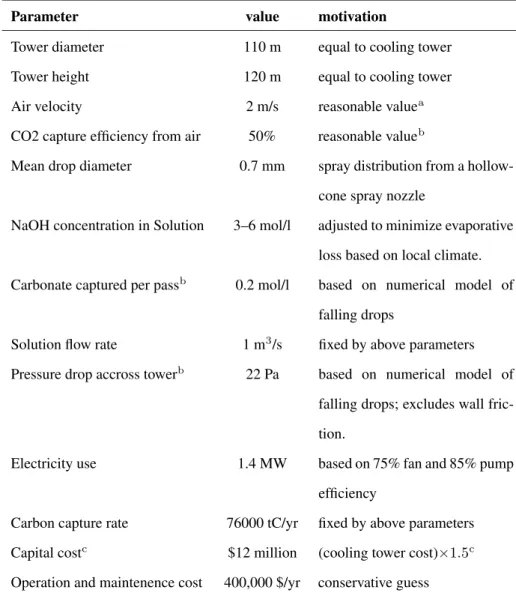
Table B.2: NaOH spray tower air capture unit: key parameters
Parameter value motivation
Tower diameter 110 m equal to cooling tower Tower height 120 m equal to cooling tower Air velocity 2 m/s reasonable valuea CO2 capture efficiency from air 50% reasonable valueb
Mean drop diameter 0.7 mm spray distribution from a hollow-cone spray nozzle
NaOH concentration in Solution 3–6 mol/l adjusted to minimize evaporative loss based on local climate. Carbonate captured per passb 0.2 mol/l based on numerical model of
falling drops
Solution flow rate 1 m3/s fixed by above parameters Pressure drop accross towerb 22 Pa based on numerical model of
falling drops; excludes wall fric-tion.
Electricity use 1.4 MW based on 75% fan and 85% pump efficiency
Carbon capture rate 76000 tC/yr fixed by above parameters Capital costc $12 million (cooling tower cost)×1.5c Operation and maintenence cost 400,000 $/yr conservative guess
a The air velocity trades off higher CO2throughput, i.e. lower capital cost, with in-creased fan energy (since fan energy goes as the square of velocity). While this value is not optimized, it falls in the likely range of the optimal value since capital costs baloon for air speeds much below this, and fan electricity costs dominate for values much above this.
bThe capture efficiency trades off higher CO2throughput, i.e. lower capital cost, with increased solution pumping. Because higher efficiencies require exponentially more energy to achieve, but low efficiencies drive up capital costs, 50% is in the likely optimal range.
c The contactor has additional cost over a cooling tower of fans and some liquid-38
of Na2CO3to NaOH by a few percent, and in general the sulfur only complicates the process. Since our proposed system doesn’t require any sulfide, we expect it to run a bit more efficiently than the kraft equivalent.
B.3.2 Temperature
In the kraft process, the slaking and causticizing steps are typically performed with a solution temperature in the range of 70-100oC. However, the solution entering this step in the proposed system will be at ambient temperature or cooler. The solution is heated by the slaking reaction; assuming a (typical) concentration of about 2 mol/l CaO added, the slaking reaction will increase the solution temperature by about 20Co, but that would only bring the solution to, perhaps, 40oC. While the equilibrium conversion efficiency of Na2CO3to NaOH is higher at lower temperatures, the kinetics become prohibitively slow. Without changing the process design to accommodate significantly longer residence times, we will have to add additional heat to the solution. Another 30Cowould bring us into the industrial range. We can do so with a liquid-to-liquid heat exchanger and a low grade heat input of (assuming the exchanger is 80% efficient) 14 kJ/mol-CO2, or about 1 GJ/ton-C.
B.3.3 Solids content
In the kraft process, the initial Na2CO3solution contains organic particles and insol-uble minerals (“dregs”) in the part-per-thousand range. The dregs impair the perfor-mance of the process and so most must be removed in a clarifier. For the proposed system, the entire dreg-removal subsystem can probably be eliminated. The source of contamination most analogous to the dregs in the proposed system is fine particles captured from the air along with the CO2. Assuming a particle concentration of 100 µg/m3and equal absorption efficiency with CO2, the particle concentration in solution will be in the range of 10 parts per million.