Publisher’s version / Version de l'éditeur:
Review of Scientific Instruments, 90, 1, 2019-01-23
READ THESE TERMS AND CONDITIONS CAREFULLY BEFORE USING THIS WEBSITE.
https://nrc-publications.canada.ca/eng/copyright
Vous avez des questions? Nous pouvons vous aider. Pour communiquer directement avec un auteur, consultez la
première page de la revue dans laquelle son article a été publié afin de trouver ses coordonnées. Si vous n’arrivez pas à les repérer, communiquez avec nous à [email protected].
Questions? Contact the NRC Publications Archive team at
[email protected]. If you wish to email the authors directly, please see the first page of the publication for their contact information.
NRC Publications Archive
Archives des publications du CNRC
This publication could be one of several versions: author’s original, accepted manuscript or the publisher’s version. / La version de cette publication peut être l’une des suivantes : la version prépublication de l’auteur, la version acceptée du manuscrit ou la version de l’éditeur.
For the publisher’s version, please access the DOI link below./ Pour consulter la version de l’éditeur, utilisez le lien DOI ci-dessous.
https://doi.org/10.1063/1.5055245
Access and use of this website and the material on it are subject to the Terms and Conditions set forth at
Thermal-wave resonant cavity signal processing
Gu, Caikang; Shen, Jun; Zhou, Jianqin; Michaelian, Kirk H.; Gieleciak, Rafal; Astrath, Nelson G. C.; Baesso, Mauro L.
https://publications-cnrc.canada.ca/fra/droits
L’accès à ce site Web et l’utilisation de son contenu sont assujettis aux conditions présentées dans le site LISEZ CES CONDITIONS ATTENTIVEMENT AVANT D’UTILISER CE SITE WEB.
NRC Publications Record / Notice d'Archives des publications de CNRC: https://nrc-publications.canada.ca/eng/view/object/?id=e0ed5b35-55df-4203-81ba-388667e356a8 https://publications-cnrc.canada.ca/fra/voir/objet/?id=e0ed5b35-55df-4203-81ba-388667e356a8
Caikang Gu1, Jun Shen1,a), Jianqin Zhou1, Kirk H. Michaelian2, Rafal Gieleciak2, Nelson G. C. Astrath3, Mauro L. Baesso3
1National Research Council Canada, Energy, Mining and Environment Research Centre, 4250
Wesbrook Mall, Vancouver, British Columbia V6T 1W5, Canada
2Natural Resources Canada, CanmetENERGY in Devon, One Oil Drive Patch, Devon, Alberta
T9G 1A8, Canada
3Departamento de Física, Universidade Estadual de Maringá, Maringá, PR 87020>900, Brazil
: The thermal>wave resonant cavity (TWRC) technique has been used for thermal diffusivity measurements by many researchers. The present study aims to reduce the uncertainty associated with TWRC signal processing (curve fitting) by means of numerical simulation and experimental verification. Simulations show that the plot of signal amplitude versus cavity length can be fitted to a simplified model reported previously when the initial fitting position is at least twice the thermal>wave diffusion length (2 ), and that the uncertainty caused by different end positions is negligible in the range 6 – 10 . Upon consideration of the simulation results, signal>to>noise ratio, and clearly defined amplitude curve shape, fitting ranges of about 2.2 – 8.0
and 2.2 – 8.7 were chosen for the experimental data. Thermal diffusivity values (1.438 ± 0.001) × 10>7 and (1.436 ± 0.001) × 10>7 m2 s>1, respectively, were obtained for distilled water, in excellent agreement with the accepted literature value. The ratio of standard deviation to the mean value is smaller than 0.07%, one order of magnitude lower than typical results reported in the literature. Similar simulation results were obtained for air and methanol as intra>cavity samples.
a)
Photopyroelectric (PPE) techniques have been successfully utilized to characterize gas, liquid, and solid materials for many years. These techniques can be categorized according to their implementation of either back> or front>detection configurations.1 Thermal>wave resonant cavity (TWRC), or thermal>wave interferometry, is a form of back>detection. In contrast with the common frequency scan employed in traditional PPE techniques, TWRC (also known as TWC) uses a thickness (cavity>length) scan, the distance scan between a thermal>wave generator and a pyroelectric detector. Because the cavity>length scan employs a selected thermal>wave
frequency, it offers two important advantages: a) the frequency>dependent instrumental transfer function is kept constant, and b) a fixed noise bandwidth is maintained throughout the
experiment. These advantages yield improved signal>to>noise ratios.2>5
Much early research work on TWRC went to the study of its basic principles and theoretical models. Early models considered only pure thermal conduction,2>4 while it was later realised that thermal radiation from the thermal>wave generator should also be taken into
account.5 The effect of the thermal radiation becomes pronounced when the cavity length is large compared with the thermal diffusion length, = / . In this expression denotes thermal diffusivity of the intra>cavity sample and f is thermal>wave frequency. Owing to the presence of the radiation, the mathematical expression for the TWRC signal turns out to be very complex and signal processing, such as curve fitting, becomes difficult. Furthermore, to obtain
, curve fitting requires knowledge of the property values (e.g., thickness, thermal properties) of the pyroelectric detector and other TWRC components. Any error in these property values will affect the accuracy of the measured .
To perform absolute measurements and eliminate the errors transferred from the property values, some researchers attempted to utilize plots of the natural logarithms of the amplitude and phase signals against cavity length. When the cavity length is not very large, these two curves are approximately linear. The slopes of the linear curves can be used to calculate according to6,7
= . (1)
In this approach, the measurement of does not require any knowledge of the property values. However, it was found that the linearity and slope of these two curves are dependent on both the beginning and end positions of the cavity>length scan, leading to an uncertainty in the measured
value.7 Thermal conduction dominates the heat transfer in the TWRC when the cavity length is not large, bringing about the linearity in these two curves. However, as the cavity length increases, the contribution of thermal radiation to the heat transfer becomes significant.5,7 As a result the end position is affected by thermal radiation and is not easily determined, since the strength of the thermal radiation is influenced by a number of factors, such as infrared emissivity and dc temperature of the thermal>wave generator. This analysis is consistent with the results of the numerical simulations reported in our previous work8 with water as the intra>cavity sample and = 20 , where the first derivatives of these two curves were calculated using the full one>dimensional TWRC theoretical model developed by Kwan et al.9 If only pure thermal conduction is considered, when the cavity length is larger than 2 , the first derivatives (i.e., the slopes) of these two curves are the same, so that can be correctly obtained. When both
thermal conduction and radiation are considered, the first derivatives appear flat only around 3 in the cavity length scan. These simulation results reveal that these two curves are not perfectly linear and that the quasi>linear range is narrow. One may conclude that it is not very
easy to delimit the linear region of these two curves; uncertainty of the linear region causes uncertainty in the slope values of these two quasi>linear curves and consequently the values of
derived from the slopes.
Absolute measurements of can be performed with less uncertainty using the methodology we developed previously.8 The one>dimensional TWRC model in Ref. 9 was simplified, taking into account both thermal conduction and radiation in heat transfer. With the simplified model, curve fitting can be carried out to determine without knowledge of the property values of the TWRC components. However, it was found that the value of the thus obtained varied with the cavity>length range used in the curve fitting. To reduce this uncertainty, the current work investigates the effects of variations in the beginning and end positions on the calculation results, establishing the proper cavity>length range for curve fitting by means of numerical simulations and experimental verification.
! " #
Figure 1 shows the experimental setup. A laser beam (Melles Griot, Model 58 GLS/GSS 301, 532.0 nm, 30 mW), modulated by a mechanical chopper (Electro>Optical Products Corp., model CH>60), was made to impinge on a surface>blackened 22> m thick aluminum foil to generate the thermal wave. The laser beam spot size on the foil was about 3 mm in diameter, much larger than the thermal diffusion length = 0.1324 mm of water at f = 2.6 Hz, thereby meeting the requirement of the one>dimensional approach. A 100> m thick PVDF film produced the TWRC signal, which was amplified by a low>noise preamplifier (Stanford Research Systems, Model SR 560) and detected by a lock>in amplifier (EG&G, Model 7260). The mechanical chopper was triggered by a TTL signal from the lock>in amplifier to improve frequency stability,
while the lock>in reference signal was obtained from the chopper. The modulation frequency varied by about 0.1%, from 2.594 to 2.597 Hz, in the experiment. The Al>foil>PVDF distance was scanned using a precise linear stage (Physik Instrument, model PLS>85, 1> m resolution). The cavity>length scan step was 5 m. Distilled water served as the intra>cavity sample. The linear stage and lock>in amplifier were controlled with a LabView program. Cavity>length scans were performed with this setup for the experimental verification.
FIG. 1. Schematic drawing of the TWRC experimental setup [the PVDF backing material (t) is not shown here]. The designed minimum distance between the thermal>wave generator (Al foil) and pyroelectric detector (PVDF) was 0.15 mm.
$ # $ $ $$
The numerical data of the TWRC amplitude signal , for the simulation were generated using the full one>dimensional theoretical model in Ref. 9:
, = !"#"#$ %& '#$($ )*$+,*$ '#$($ -./"$ '#"("+ 0
!$#$%& ' #"(" 1
/"$2*$34"+3*$24"+0 5'6' #4(4!"#" 73*$ %& ' #"("+2*$8/"$ %+ ' #"(" &. ' #"("9:
In Eq. (2), S(f) is an instrumental factor which is constant for a fixed frequency f, and ;< = 1 + ? / <. < = </ is the thermal>wave diffusion length, αjis the thermal diffusivity, and Lj is the thickness of material j. Subscripts @ = A, B, C, D represent the Al foil acting as a thermal>wave generator, the intra>cavity sample, pyroelectric detector, and detector backing material, respectively, as shown in Fig. 1. The other quantities are defined by
EF< =GGJHIIHJ= HJ,
KF< = 1 − EF< + 1 + EF< M&.IHNH, OF< = 1 + EF< + 1 − EF< M&.IHNH,
PF< = OF< + KF<M&.IJNJ, QF< = OF< − KF<M&.IJNJ,
where M< = R<S <T< is the thermal effusivity. kj, S < and ρj are the thermal conductivity, specific heat, and density of material j, respectively. = 4;V WZXY is the heat transfer
coefficient, where σ = 5.6697 × 10>8 Wm>2K>4 is the Stefan>Boltzmann constant; εs (0 ≤ V ≤ 1) is the infrared emissivity of material s; Tsdc is the dc component of the temperature of the thermal wave generator. For water as an intra>cavity sample, as noted in Ref. 10, the water layer adjacent to the thermal>wave generator is the main source of the thermal radiation, and the infrared emissivity εs is between 0.96 and 0.99. Selecting εs = 0.97 and WXY = 21 °C, one obtains
H about 5.6 Wm>2K>1. The amplitude data were generated for numerical simulation using the parameters cavity length range 1 – 10 (0.1324 – 1.324 mm), a step size of 0.04 , f = 2.6 Hz,
= 5.6 Wm>2K>1, and = 1.431 × 10>7 m2 s>1.
, = S \2 2 + 8√2 MBM −B BA?_` B B+4a+ 16MB 2M−2BB. (3)
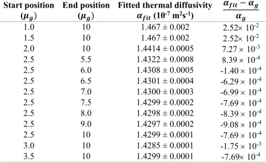
Here S is a constant with a fixed f. Table I presents the results for water with a series of start and end positions for the curve fitting. It is clearly evident that the relative difference, compared with the expected value of the thermal diffusivity cd (column 4), is less than 1% when the start position is 2 or beyond. This is consistent with the conclusion that the simplified model is valid when the cavity length is greater than or equal to 2 . Table I also shows, with the start position at 2.5 , that variation in the end position between 6 and 10 hardly affects the fitted thermal diffusivity values; these fitted values are slightly smaller than the expected value. In other words, the uncertainty caused by the different end positions is negligible.
Table I. Numerical simulation results for water as an intra>cavity sample: fitted thermal diffusivity values c Fe at various start and end positions for curve fitting. Parameters used for the simulation: = 1.431 × 10>7 m2 s>1, f = 2.6 Hz, = 5.6 Wm>2K>1. $ %fd & %fd ' & & (() cghi%*+, - *. cghi− cd cd 1.0 10 1.467 ± 0.002 2.52× 10>2 1.5 10 1.467 ± 0.002 2.52× 10>2 2.0 10 1.4414 ± 0.0005 7.27 × 10>3 2.5 5.5 1.4322 ± 0.0008 8.39 × 10>4 2.5 6.0 1.4308 ± 0.0005 >1.40 × 10>4 2.5 6.5 1.4301 ± 0.0004 >6.29 × 10>4 2.5 7.0 1.4300 ± 0.0003 >6.99 × 10>4 2.5 7.5 1.4299 ± 0.0002 >7.69 × 10>4 2.5 8.0 1.4298 ± 0.0002 >8.39 × 10>4 2.5 9.0 1.4297 ± 0.0002 >9.08 × 10>4 2.5 10 1.4299 ± 0.0001 >7.69 × 10>4 3.0 10 1.4285 ± 0.0001 >1.75 × 10>3 3.5 10 1.4299 ± 0.0001 >7.69× 10>4
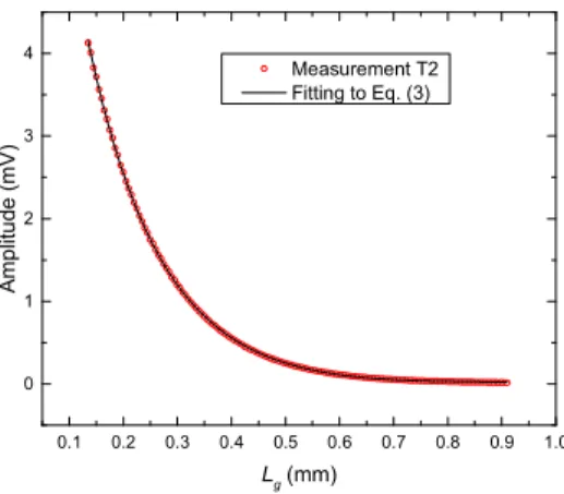
In the numerical simulation, the effect of noise, which naturally exists in the experimental measurement, has not been considered. When dealing with experimental data, noise must be taken into account. In cases where the cavity length is short, the signal amplitude is strong and the signal>to>noise ratio (S/N) is high. By contrast, the signal becomes weak and S/N is low when the cavity length is greater. On one hand, to reduce the effect of noise, it is better to choose the data with a short cavity>length range for the curve fitting. On the other hand, the curve fitting essentially fits the theoretical model to the curve shape of the experimental data; therefore, the choice of an adequate cavity>length range with a clear curve shape is necessary for proper curve fitting. Based on this reasoning, the fitting ranges in the experimental verification were about 2.2 – 8.0 (shown in Fig. 2) and 2.2 – 8.7 . The values thus obtained for the six
measurements were (1.438 ± 0.001) × 10>7 and (1.436 ± 0.001) × 10>7 m2 s>1, respectively. Compared with the literature value = 1.431 × 10>7 m2 s>1,11 the relative differences are only about 0.49% and 0.35%, respectively. This indicates the high accuracy of the measurements and the validity of the curve>fitting method. Furthermore, the six measurements T1 – T6 were carried out over a two>day period (three measurements per day with a new sample each day), and the ratios of the standard deviation to the mean value were smaller than 0.07%. This compares quite favorably with typical relative errors for thickness (cavity length) scans of about 0.8 – 3%;12 stated differently, the precision in the present work is better by at least an order of magnitude. The good reproducibility of the current experiment is shown in Fig. 3, where the six measured signal curves are seen to be practically identical. This excellent precision / repeatability may be attributed to the very stable mechanical chopper frequency during the measurements, in which the chopper was controlled by the lock>in amplifier.
!
"
#
FIG. 2. Experiment T2 data fitted to Eq. (3). Fitted = 1.436 × 10>7 m2 s>1 with fitting length range about 2.2 – 8.0 and a correlation coefficient R2 = 0.9997.
! " # ! " #
FIG. 3. Amplitude signals , for six measurements: T1 – T3 on the first day and T4 – T6 on the second day. Inset shows the details of the six measurements with < 0.11 mm.
Similar conclusions are reached with other gas or liquid materials (e.g., air or methanol) as the intra>cavity samples. Table II shows the simulation results for air with the thermal diffusivity and emissivity values = 2.224×10>5 m2 s>1 and V ≈ 0.05 reported in Refs. 5 and 10, respectively. Simulation results for methanol are presented in Table III. Ref. 11 reports the
thermal diffusivity of methanol as = 9.98×10>8 m2 s>1, while Ref. 10 gives V ≈ 0.4. W XY = 21 °C was used for the calculation of values for Tables II and III. These two tables show that the thermal diffusivity cd value can be obtained with a relative difference smaller than 1.5% compared with the expected value when the start position is greater than 2 . With the start position set at 2.5 , variation of the end position from 6 to 10 hardly affects the thermal diffusivity values obtained by curve fitting.
Table II. Numerical simulation results for air as an intra>cavity sample: fitted thermal diffusivity values c Fe at various start and end positions for curve fitting. Parameters for the simulation: = 2.224 × 10>5 m2 s>1, f = 20 Hz, = 0.3 Wm>2K>1. $ %fd & %fd ' & & (() cghi%*+/ - *. cghi− cd cd 1.0 10 2.362 ± 0.005 6.21× 10>2 1.5 10 2.341 ± 0.005 5.26 × 10>2 2.0 10 2.257 ± 0.002 1.48 × 10>2 2.5 6 2.2208 ± 0.0009 >1.44 × 10>3 2.5 7 2.2197 ± 0.0006 >1.93 × 10>3 2.5 8 2.2196 ± 0.0005 >1.98 × 10>3 2.5 9 2.2194 ± 0.0005 >2.07 × 10>3 2.5 10 2.2193 ± 0.0004 >2.11 × 10>3 3.0 10 2.2159 ± 0.0001 >3.64 × 10>3 3.5 10 2.223 ± 0.009 >4.50× 10>4
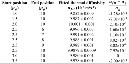
Table III. . Numerical simulation results for methanol as an intra>cavity sample: fitted thermal diffusivity values at various start and end positions for curve fitting. Parameters for the
simulation: = 9.98 × 10>8 m2 s>1, f = 2.6 Hz, = 2.3 Wm>2K>1. $ %fd & %fd ' & & (() cghi %*+0 - *. cghi− cd cd 1.0 10 9.852 ± 0.009 >1.28×10>2 1.5 10 9.987 ± 0.002 >7.01×10>4 2.0 10 10.001 ± 0.001 2.10×10>3 2.5 6 9.996 ± 0.003 1.60×10>3 2.5 7 9.991 ± 0.002 1.10×10>3 2.5 8 9.988 ± 0.001 8.02×10>4 2.5 9 9.988 ± 0.001 8.02×10>4 2.5 10 9.9879 ± 0.0009 7.92×10>4 3.0 10 9.980 ± 0.001 0 3.5 10 9.978 ± 0.001 >2.00×10>4
The thermal diffusivity values of gases and liquids generally fall within particular ranges. Specifically, thermal diffusivities are on the order of 10>5 m2 s>1 for a number of gases and 10>7 m2 s>1 for liquids (e.g., common solvents);11 thermal diffusion lengths can be roughly estimated based on these values. Since the cavity length range for thermal diffusivity
measurement is wide (typically 2 to 10 ), it is generally not difficult to select the measurement lengths, based on this knowledge of the estimated , for a new sample. With the simplified model in Eq. (3) and the cavity length ranges discussed above, the thermal diffusivity can be measured more accurately as compared with the curve fitting using the full model in Eq. (2), which requires knowledge of the property values of the pyroelectric detector and other TWRC components. For instance, alternative fuels blended with ultralow sulfur diesel were measured precisely in this way.13
The conclusions drawn from Tables I – III are expected to be broadly applicable for thermal diffusivity measurements of gases and liquids. In a TWRC, heat transfer is the combination of thermal conduction and radiation. Thermal conduction contributes more as compared with thermal radiation when the cavity length is short. Consequently, thermal diffusivity can be measured correctly with short cavity length ranges, such as 2.5 – 6 . The effect of thermal radiation becomes more significant as the cavity length increases. As a result, longer cavity lengths, extending from 2.5 – 8 , may be required in the measurement of the parameters related to radiation, i.e., H or εs. Radiation>related parameters are not easy to measure, and are currently under investigation.
In summary, processing of the TWRC signal for gas and liquid intra>cavity samples is discussed in detail in this article. Numerical simulation shows that the starting position for curve fitting should not be less than 2 . To obtain optimal results, both signal>to>noise ratio and the clear presence of a well>defined amplitude>distance curve should be considered during selection of the curve fitting range. Following these principles, variations due to the use of different positions are negligible and highly accurate, precise experimental results are achievable.
( 1
1. D. Dadarlat and C. Neamtu, Acta Chim. Slov. /2, 225 (2009).
2. A. Mandelis, and A. Matvienko, “Photopyroelectric thermal>wave cavity devices ─ 10 years later” in Pyroelectric Materials and Sensors, edited by D. Rémiens (Research Signpost, Kerala, India, 2007).
3. E. Marín and H. Vargas, “Recent developments in thermal wave interferometry for gas analysis” in Thermal Wave Physics and Related Photothermal Techniques: Basic Principles and Recent
Developments, edited by E. M. Moares (Transworld Research Network, Kerala, India, 2009).
4. J. Shen and A. Mandelis, Rev. Sci. Instrum. 22, 4999 (1995).
5. J. Shen, A. Mandelis, and H. Tsai, Rev. Sci. Instrum. 23, 197 (1998).
6. J. A. Balderas>López, A. Mandelis, and J. A. Garcia, Rev. Sci. Instrum. ,*, 2933 (2000). 7. S. Delenclos, D. Dadarlat, N. Houriez, S. Longuemart, C. Kolinsky, and A. Hadj Sahraoui,
Rev. Sci. Instrum. ,0, 024902 (2007).
8. J. Shen, J. Zhou, C. Gu, S. Neill, K. H. Michaelian, C. Fairbridge, N. G. C. Astrath, and M. L. Baesso, Rev. Sci. Instrum. 04, 124902 (2013).
9. C. H. Kwan, A. Matvienko, and A. Mandelis, Rev. Sci. Instrum. 78, 104902 (2007). 10. A. Matvienko and A. Mandelis, Int. J. Thermophys. -2, 837 (2005).
11. S.E. Bialkowski, Photothermal Spectroscopy Methods for Chemical Analysis, (Wiley, New York, 1996).
12. A. O. Guimaraes, F. A. L. Machado, E. C. da Silva, and A. M. Mansanares, Thermochimica Acta /-,, 125 (2012).
13. T. Petrucci, K. H. Michaelian, R. Gieleciak, J. Shen, J. Zhou, C. Gu, W. S. Neill, M. L. Baesso, L. C. Malacarne, N. G. C. Astrath, Energy & Fuels, 31, 13775 (2017).
![FIG. 1. Schematic drawing of the TWRC experimental setup [the PVDF backing material (t) is not shown here]](https://thumb-eu.123doks.com/thumbv2/123doknet/14029333.457983/6.918.381.579.397.619/schematic-drawing-twrc-experimental-setup-pvdf-backing-material.webp)