HAL Id: hal-02991325
https://hal.archives-ouvertes.fr/hal-02991325
Submitted on 10 Nov 2020
HAL is a multi-disciplinary open access
archive for the deposit and dissemination of
sci-entific research documents, whether they are
pub-lished or not. The documents may come from
teaching and research institutions in France or
abroad, or from public or private research centers.
L’archive ouverte pluridisciplinaire HAL, est
destinée au dépôt et à la diffusion de documents
scientifiques de niveau recherche, publiés ou non,
émanant des établissements d’enseignement et de
recherche français ou étrangers, des laboratoires
publics ou privés.
Orbiter
S. Solanki, J. del Toro Iniesta, J. Woch, A. Gandorfer, J. Hirzberger, A.
Alvarez-Herrero, T. Appourchaux, V. Martínez Pillet, I. Pérez-Grande, E.
Sanchis Kilders, et al.
To cite this version:
S. Solanki, J. del Toro Iniesta, J. Woch, A. Gandorfer, J. Hirzberger, et al.. The Polarimetric and
Helioseismic Imager on Solar Orbiter. Astronomy and Astrophysics - A&A, EDP Sciences, 2020, 642,
pp.A11. �10.1051/0004-6361/201935325�. �hal-02991325�
Astronomy& Astrophysics manuscript no. main ESO 2019c March 15, 2019
The Polarimetric and Helioseismic Imager on Solar Orbiter
S.K. Solanki
1, 15?, J.C. del Toro Iniesta
2, J. Woch
1, A. Gandorfer
1, J. Hirzberger
1, A. Alvarez-Herrero
3,
T. Appourchaux
4, V. Martínez Pillet
5, I. Pérez-Grande
6, E. Sanchis Kilders
7, W. Schmidt
9, J.M. Gómez Cama
10,
H. Michalik
11, W. Deutsch
1, G. Fernandez-Rico
1, 6, B. Grauf
1, L. Gizon
1, 16, K. Heerlein
1, M. Kolleck
1, A. Lagg
1,
R. Meller
1, R. Müller
1, U. Schühle
1, J. Staub
1, K. Albert
1, M. Alvarez Copano
1, U. Beckmann
1, J. Bischo
ff
1,
D. Busse
1, R. Enge
1, S. Frahm
1, D. Germerott
1, L. Guerrero
1, B. Löptien
1, T. Meierdierks
1, D. Oberdorfer
1,
I. Papagiannaki
1, S. Ramanath
1, J. Schou
1, S. Werner
1, D. Yang
1, A. Zerr
1, M. Bergmann
1, J. Bochmann
1,
J. Heinrichs
1, S. Meyer
1, M. Monecke
1, M.-F. Müller
1, M. Sperling
1, D. Álvarez García
2B. Aparicio
2, M. Balaguer
Jiménez
2, L.R. Bellot Rubio
2, J.P. Cobos Carracosa
2, F. Girela
2, D. Hernández Expósito
2, M. Herranz
2, P. Labrousse
2,
A. López Jiménez
2, D. Orozco Suárez
2, J.L. Ramos
2, J. Barandiarán
3, L. Bastide
3, C. Campuzano
3, M. Cebollero
3,
B. Dávila
3, A. Fernández-Medina
3, P. García Parejo
3, D. Garranzo-García
3, H. Laguna
3, J.A. Martín
3, R. Navarro
3,
A. Núñez Peral
3, M. Royo
3, A. Sánchez
3, M. Silva-López
3, I. Vera
3, J. Villanueva
3, J.-J. Fourmond
4, C. Ruiz de
Galarreta
4, M. Bouzit
4, V. Hervier
4, J.C. Le Clec’h
4, N. Szwec
4, M. Chaigneau
4, V. Buttice
4, C. Dominguez-Tagle
4, 12,
A. Philippon
4, P. Boumier
4, R. Le Cocguen
14, G. Baranjuk
4, A. Bell
9, Th. Berkefeld
9, J. Baumgartner
9, F. Heidecke
9,
T. Maue
9, E. Nakai
9, T. Scheiffelen
9, M. Sigwarth
9, D. Soltau
9, R. Volkmer
9, J. Blanco Rodríguez
8, V. Domingo
8,
A. Ferreres Sabater
7, J.L. Gasent Blesa
8, P. Rodríguez Martínez
8, D. Osorno Caudel
7, J. Bosch
10, A. Casas
10,
M. Carmona
10, A. Herms
10, D. Roma
10, G. Alonso
6, A. Gómez-Sanjuan
6, J. Piqueras
6, I. Torralbo
6, B. Fiethe
11,
Y. Guan
11, T. Lange
11, H. Michel
11, J.A. Bonet
12, S. Fahmy
13, D. Müller
13, and I. Zouganelis
13(Affiliations can be found after the references) Received December 31, 2018; accepted January 1, 2019
ABSTRACT
Aims.This paper describes the Polarimetric and Helioseismic Imager on the Solar Orbiter mission (SO/PHI), the first magnetograph and
helioseis-mology instrument to observe the Sun from outside the Sun-Earth line. It is the key instrument meant to address the top-level science question: How does the solar dynamo work and drive connections between the Sun and the heliosphere? SO/PHI will also play an important role in answering the other top-level science questions of Solar Orbiter, as well as hosting the potential of a rich return in further science.
Methods.SO/PHI measures the Zeeman effect and the Doppler shift in the Fe i 617.3 nm spectral line. To this end, the instrument carries out
narrow-band imaging spectro-polarimetry using a tunable LiNbO3Fabry-Perot etalon, while the polarisation modulation is done with liquid crystal
variable retarders (LCVRs). The line and the nearby continuum are sampled at 6 wavelength points and the data are recorded by a 2k × 2k CMOS detector. To save valuable telemetry, the raw data are reduced on board, including being inverted under the assumption of a Milne-Eddington atmosphere, although simpler reduction methods are also available on board. SO/PHI is composed of two telescopes; one, the Full Disc Telescope (FDT), covers the full solar disc at all phases of the orbit, while the other, the High Resolution Telescope (HRT), can resolve structures as small as 200 km on the Sun at closest perihelion. The high heat load generated through proximity to the Sun is greatly reduced by the multilayer-coated entrance windows to the two telescopes that allow less than 4% of the total sunlight to enter the instrument, most of it in a narrow wavelength band around the chosen spectral line.
Results.SO/PHI was designed and built by a consortium having partners in Germany, Spain and France. The flight model was delivered to Airbus
Defence and Space, Stevenage, and successfully integrated into the Solar Orbiter spacecraft. A number of innovations were introduced compared with earlier space-based spectropolarimeters, thus allowing SO/PHI to fit into the tight mass, volume, power and telemetry budgets provided by the Solar Orbiter spacecraft and to meet the (e.g., thermal) challenges posed by the mission’s highly elliptical orbit.
Key words. Instrumentation: polarimeters – Techniques: imaging spectroscopy – Techniques: polarimetric – Sun: photosphere – Sun: magnetic fields – Sun: helioseismology
1. Introduction
The Sun’s magnetic field is to a large extent responsible for driv-ing a host of active phenomena, rangdriv-ing from sunspots at its surface to coronal mass ejections propagating through the he-liosphere (Solanki et al. 2006; Wiegelmann et al. 2014). The magnetic field also couples the various layers of the solar at-mosphere, connecting the solar surface to the chromosphere and
? Corresponding author: Sami K. Solanki
e-mail: [email protected]
corona and transporting the energy needed to heat the upper at-mosphere and to accelerate the solar wind. Hence it is imperative to measure the Sun’s magnetic field if we are to follow, under-stand and model the active phenomena on the Sun and in the heliosphere. Consequently, polarimeters aimed at measuring the magnetic field have become increasingly central to solar physics, although only few have flown in space so far, mainly because of their complexity and the technical challenges involved.
Whereas a polarimeter can measure the field in the solar at-mosphere, usually close to the solar surface, the magnetic field
itself is produced in the solar interior, which is opaque to elec-tromagnetic radiation (e.g., Charbonneau 2010). To gain insight into the structures and forces acting there we must take recourse to helioseismology, i.e. the study of the acoustic waves that are excited profusely in the convection zone of the Sun (e.g., Gizon & Birch 2005; Basu 2016).
In this paper we describe the SO/PHI instrument, the Po-larimetric and Helioseismic Imager on board the Solar Orbiter Mission (Garcia-Marirrodriga 2019). This instrument aims at achieving both tasks outlined above, i.e. measuring the magnetic field at the solar surface and probing the solar interior by mea-suring oscillations seen in the line-of-sight velocity. It is one of the suite of remote sensing instruments on Solar Orbiter, the first medium class mission of the European Space Agency’s Cosmic Vision program (Müller et al. 2019).
SO/PHI is a magnetograph, the fifth instrument aimed at measuring the solar magnetic field in space, after SOHO/MDI
(Scherrer et al. 1995), SDO/HMI (Schou et al. 2012b),
Hin-ode/SP (Lites et al. 2013) and Hinode/NFI (Tsuneta et al.
2008b). It is also an instrument designed to do
helioseis-mology from space, after SOHO/MDI (Scherrer et al. 1995),
SOHO/GOLF (Gabriel et al. 1995), SOHO/VIRGO (Fröhlich
et al. 1995), SDO/HMI (Schou et al. 2012b) and Picard
(Cor-bard et al. 2013).
The capabilities of SO/PHI differ from these earlier instru-ments in a number of ways. Firstly, SO/PHI is the first magne-tograph that will observe the Sun from outside the Sun-Earth line. Secondly, it is the first such instrument planned to leave the ecliptic and get a clear view of the solar poles. It has two channels, one to observe the full solar disc and another to ob-serve the Sun at high resolution (which is qualitatively similar
to SOHO/MDI, although SO/PHI will reach considerably higher
spatial resolution around perihelion).
The paper is structured as follows. In Section 2 the science objectives of the SO/PHI instrument are given, which signifi-cantly overlap with those of the Solar Orbiter mission as a whole. An overview of the instrument is provided in Section 3, with more details on various aspects of the instrument being provided in Section 4 (optical unit), Section 5 (electronics), Section 6 (in-strument characterisation and calibration) and Section 7 (science operations). Finally, a summary is given in Section 8.
2. Science objectives
2.1. Top level science questions
The overarching science goal of Solar Orbiter is to answer the question: How does the Sun create and control the heliosphere? This umbrella encompasses 4 top-level science questions:
1. How does the solar dynamo work and drive connections be-tween the Sun and the heliosphere?
2. What drives the solar wind and where does the coronal mag-netic field originate from?
3. How do solar transients drive heliospheric variability? 4. How do solar eruptions produce energetic particle radiation
that fills the heliosphere?
A more detailed discussion of these questions is given in the Solar Orbiter Red Book (see Marsden et al. 2011) and in Müller et al. (2013).
The magnetograms and helioseismic data recorded by SO/PHI will provide significant, often vital information to an-swer the above questions. We consider these questions individu-ally in Sects. 2.2, 2.3, 2.4 and 2.5, respectively and consider how
SO/PHI will help to address them. Finally, in Section 2.6 we also present and discuss additional science questions. SO/PHI is unique in being the first ever magnetograph and helioseismology instrument to observe the Sun from outside the Sun-Earth line, enabling it to do science that goes beyond the specific aims iden-tified in the Solar Orbiter Red Book. This will allow SO/PHI to greatly enhance the science output from Solar Orbiter.
2.2. How does the solar dynamo work and drive connections between the Sun and heliosphere?
The magnetic field of the Sun is, in one way or another, the main driver of solar activity. It structures the solar chromosphere and corona and is responsible for coronal heating, it leads to flares and CMEs besides playing an important role in driving the so-lar wind (Solanki et al. 2006; Priest 2014). The magnetic field, its large-scale structure and its roughly 11-year cycle (e.g. Hath-away 2010), are clearly results of a dynamo mechanism (e.g., Charbonneau 2010; Cameron et al. 2017). Nonetheless, there are still many open questions surrounding the nature of this dynamo. For example, there is no consensus on the depth below the solar surface at which the dynamo responsible for sunspots and the solar cycle is located; there is not even agreement if it is mainly restricted to the overshoot layer below the convection zone, or if it is distributed over (a part of) the convection zone (Babcock 1961; Leighton 1969; Cameron & Schüssler 2015). Proposals for the location of the dynamo cover the two main radial shear layers, one at the bottom of the convection zone and one near the solar surface (Howe 2009; Brandenburg 2005), cf. Charbonneau (2013). There is also a debate on whether the dynamo responsi-ble for the solar cycle is the only solar dynamo, or if a separate small-scale turbulent dynamo is also acting closer to the solar surface (Vögler & Schüssler 2007). The variety of approaches and models of the dynamo responsible for the solar cycle have been reviewed by Charbonneau (2010, 2014), who also discusses some of the major open questions.
Critical unknowns entering solar dynamo models are the structures of the Sun’s magnetic and flow fields at high latitudes. In particular, the poloidal field at solar activity minimum is the source of the toroidal magnetic flux that dominates during the high activity phase of the solar cycle (Babcock 1961; Cameron & Schüssler 2015). Thus, the polar magnetic flux at activity min-imum is the parameter that best predicts the strength of the next solar cycle (e.g. Schatten et al. 1978; Petrovay 2010), so that it clearly plays a critical role in seeding the solar dynamo. How-ever, because all magnetographs built so far have observed from within the ecliptic plane, they have only limited sensitivity to the polar field. High-resolution images and magnetograms of the
polar region taken with the SOT/SP on board Hinode (Tsuneta
et al. 2008a,b; Shiota et al. 2012) show a rich and evolving land-scape of magnetic features around the poles. However, at the poles themselves the results are less clear-cut, largely due to the very strong foreshortening, but also because the nearly vertical magnetic features close to the poles are almost perpendicular to the line-of-sight (LOS), leading to a small signal in the magne-tograms showing the line-of-sight magnetic field. Measurements and models of solar polar magnetic fields are reviewed by Petrie (2015).
The overarching question in the title of this subsection leads to a series of more detailed questions: How is the surface mag-netic field transported in latitude by the meridional flow? Are there multiple cells in latitude? Where is the return flow located and what role does it play in the evolution of the field? What is
evo-lution of the field? How is the field reprocessed at high latitudes? Is there a significant local solar dynamo? In the following sub-sections we will discuss these questions and demonstrate how SO/PHI will address them, especially by using the high latitude passes.
2.2.1. What is the structure of the solar rotation?
The transport of the magnetic flux near the poles by convection,
differential rotation and meridional flows is important for the
po-larity reversal of the global magnetic field (see Wang et al. 1989; Sheeley 1991; Makarov et al. 2003; Jiang et al. 2014). To gain insight into surface magnetic flux transport, the driving flows must be studied and the motions of the magnetic flux elements followed.
Thanks to global helioseismology (e.g.
Christensen-Dalsgaard 2002; Basu 2016), the solar differential rotation has
been mapped as a function of latitude and radius throughout most of the Sun (Schou et al. 1998). However, uncertainties in the results become large at high latitudes, so that there is a gap
in our knowledge for heliographic latitudes above ≈ 70◦.
While current data above ≈ 70◦heliographic latitude are
un-certain, the bands of faster and slower rotation (torsional
oscil-lations) moving toward the poles above 45◦latitude show a very
dynamic behaviour in the near-polar regions (Howe et al. 2018). An alternative to global helioseismology is local helioseis-mology (e.g. Gizon & Birch 2005), which aims to measure the 3D velocity vectors of the material flows in the solar interior, allowing studies of convective, rotational and meridional flows, as well as of the subsurface structures of sunspots and active re-gions. Local helioseismology, using SO/PHI observations will enable the study of all major subsurface flows at high helio-graphic latitudes. By repeating both, global and local helioseis-mology measurements over the course of the mission, it will be possible to deduce solar-cycle variations in these flows.
Fig. 1. Stereoscopic helioseismology. Numerical simulations showing the spatial sensitivity of helioseismic holography to the meridional flow at latitude 75◦
and radius 0.7R . The resolution is poor when using only
observations of solar oscillations in the equatorial plane (left panel, data coverage indicated in red). The resolution approaches the diffraction limit of λ/2 ≈ 38 Mm when combining the previous data with observa-tions from a line of sight inclined by 35◦
. The noise in the measurements may be very high; it depends on the total duration of the observations. See Gizon et al. (2018) for a discussion of signal and noise in helioseis-mic holography.
To this end SO/PHI will enable us to use stereoscopic he-lioseismology by combining SO/PHI data with Doppler mea-surements from Earth-based, or Earth-orbiting instruments, e.g.,
GONG (Harvey et al. 1996) or SDO/HMI (see Fig. 1). Local
lioseismic inversions from techniques such as time-distance
he-lioseismology, or helioseismic holography will be able to probe deep into the Sun using observations from widely separated van-tage points, because skip distances (distances between the sur-face end points of the ray paths) of order half a circumference will at last become accessible (Löptien et al. 2015). This will be important for probing the tachocline at the base of the convection zone, where the dynamo has been surmised to be situated.
A discussion of the helioseismic investigations that can be done with SO/PHI has been published by Löptien et al. (2015).
During the high-latitude phases of the mission’s orbit, SO/PHI will also determine surface flows at and around the poles with unprecedented accuracy by tracking small-scale features, such as granules or magnetic elements (e.g., using local cor-relation tracking; November & Simon 1988) complemented by Doppler-shift measurements. This will be possible thanks to the high spatial resolution achieved by the High Resolution Tele-scope (HRT, see Section 4.2.1) over most of the orbit. As Fig. 2
shows, although granules are hard to identify at 7◦ from the
so-lar limb (which is the most favourable angle at which a soso-lar
pole can be seen from Earth), they become clearly visible at 35◦,
close to the highest heliographic latitude to be reached by Solar Orbiter. Also, magnetic features are far more clearly visible in
Stokes V at 35◦than at 7◦from the limb.
2.2.2. What is the structure of the meridional flow?
Local helioseismology is also able to measure the meridional flow and provides evidence for temporal variations (Liang et al. 2018; Komm et al. 2018; Chen & Zhao 2017; Böning et al. 2017). Unfortunately the various measurements continue to be inconsistent leading to significant uncertainty regarding the dy-namics near the poles. SO/PHI will make a fundamental contri-bution to our understanding of the solar dynamo by observing the meridional flow in the polar regions using helioseismic tech-niques.
2.2.3. How is magnetic flux reprocessed at high solar latitudes?
SO/PHI will explore, from vantage points at different helio-graphic latitudes, the transport processes of magnetic flux from the activity belts towards the poles and the interaction of this flux with the already present polar magnetic field. This includes
the often small-scale cancellation effects whose combined
ef-fect causes the reversal of the dominant polarity at the poles leading to the next activity cycle. SO/PHI will use a multi-pronged approach, employing Doppler, proper motion and helio-seismic measurements to determine convective flows, the pole-ward meridional flow at the surface and surface differential ro-tation at high latitudes. It will follow the short-term evolution of individual magnetic features at high latitudes, but also the evolu-tion of the distribuevolu-tion of the field at the poles over the lifetime of the mission.
SO/PHI will obtain a much clearer view of the solar polar magnetic fields during the high latitude passes than currently possible. This will be true particularly in the later phases of the mission when the highest heliographic latitudes will be reached.
2.2.4. Is a small-scale turbulent dynamo process acting on the Sun?
In addition to the cancellation effects just mentioned, MHD
1•104 2•104 3•104 4•104 5•104 IC 700 750 800 850 900 950 X [arcsec] −50 0 50 Y [arcsec]
Angle from Limb: 35˚ vs. 7˚
IC IC IC −0.006 −0.004 −0.002 0.000 0.002 0.004 0.006 V/I C 700 750 800 850 900 950 X [arcsec] −50 0 50 Y [arcsec]
Angle from Limb: 35˚ vs. 7˚
V/IC V/IC
V/IC
Fig. 2. Continuum intensity map (upper panel) and Stokes V map (lower panel) of a quiet-Sun region near the limb observed by Hinode/SOT/SP. The inserts at 7◦
and 35◦
from the limb (red crosses) are centred close to the maximum viewing angles of the solar poles from the ecliptic and from Solar Orbiter, respectively. The enhanced contrast signal at 35◦
viewing angle allows for a superior determination of the atmospheric parameters. The grey scales of both inserts cover the same dynamic range, but are individually centred to their mean intensity values.
in the solar interior and at its surface (Brun et al. 2004; Vögler & Schüssler 2007; Rempel 2014). In spite of tantalising obser-vational evidence for a surface dynamo (e.g., Danilovic et al. 2010, 2016; Buehler et al. 2013; Lites et al. 2014) and for a sin-gle source of all magnetic flux on the Sun (e.g., Parnell et al. 2009), the case for either local dynamo action or a single source for all solar magnetic flux is still not settled.
Here SO/PHI will be able to make a unique contribution to determining the origin of small-scale fields by observing the
Sun from different latitudinal vantage points. By reaching
helio-graphic latitudes higher than 25◦SO/PHI will measure magnetic
fields equally reliably at all latitudes on the Sun (Martínez Pillet 2007). By measuring the properties of freshly emerged small-scale magnetic features over all heliographic latitudes, SO/PHI will be able to distinguish between their formation by a small-scale turbulent dynamo, which is independent of solar rotation,
or by the differential rotation-driven global solar dynamo. In the
former case the emergence rate and properties of the small scale magnetic features should be largely independent of heliographic latitude, while in the latter case there should be a clear latitu-dinal dependence. If, e.g., smaller magnetic features are mainly formed by a small-scale dynamo, while larger features carrying more magnetic flux per feature are largely a product of the global dynamo, SO/PHI will provide an estimate for where the
mag-netic flux or size boundary between such features of different
origin lies.
2.3. What drives the solar wind and where does the coronal magnetic field originate?
2.3.1. Pinpoint the origins of the solar wind streams and the heliospheric magnetic field
The origin and acceleration of the solar wind is intimately linked to the magnetic field (Marsch 2006). Of the two types of solar wind, the rather homogeneous and steady fast wind (with speeds
in excess of 600 km s−1) originates in the open magnetic
config-uration of coronal holes. Thus, Tu et al. (2005) have identified coronal funnels anchored in the magnetic network as the source regions of the fast wind.
The source of the highly variable — in speed, composi-tion and charge state — slow wind component is more com-plex and less certain, although its origin tends to lie in the dom-inantly closed-field regions. It has been proposed to originate from boundary layers of small coronal holes, from the tops of streamers (Sheeley et al. 1997), or from opening loops (Fisk et al. 2003). Embedded in the solar wind are magnetic field lines that are dragged out with it. One of the aims of Solar Orbiter is to determine the origins of both, the solar wind plasma and the em-bedded magnetic field.
The Solar Orbiter mission will establish the possibility of de-tecting slow solar wind streams by its in-situ instruments in co-ordination with measurements of the photospheric field below the wind stream detection site.
SO/PHI will provide the distribution and evolution of the vector magnetic and velocity fields in the photosphere at a spa-tial and temporal resolution commensurate with the other re-mote sensing instruments on board Solar Orbiter (Auchère et al. 2019). From the data products delivered by SO/PHI, the mag-netic field geometry in the upper solar atmosphere responsible for accelerating the solar wind can be derived (Schrijver & De Rosa 2003; Wiegelmann & Sakurai 2012; Wiegelmann et al. 2014).
Thus, SO/PHI will supply the magnetic and dynamic bound-ary conditions for the plasma processes observed in the higher layers of the solar atmosphere by the EUI, SPICE, Metis and STIX instruments (Rochus et al. 2019; SPICE Consortium et al. et al. 2019; Antonucci et al. 2019; Krucker 2019) on board Solar Orbiter and in the inner heliosphere by SoloHI (Howard et al. 2019). In addition, such plasma processes will be measured in situ by EPD, SWA, MAG and RPW (Rodríguez-Pacheco et al. 2019; Owen 2019; Horbury 2019; Maksimovic et al. 2019) In addition, studies of the dynamical connections between the so-lar interior and the atmosphere will benefit from the subsurface flows derived from local helioseismology with SO/PHI (Duvall et al. 1993; Gizon & Birch 2005).
How is the polar high-speed wind generated and how does this relate to the polar plume phenomenon? There are still considerable gaps in our knowledge of how the fast solar wind is accelerated. Thus, although it was shown that the wind emanates mainly from coronal funnels, network regions where the field lines are open and reach out into the heliosphere (Tu et al. 2005), their structure and properties are still only vaguely known. Ob-servations from high latitudes will uncover the detailed magnetic structure responsible for these features in the polar coronal holes. Due to the cos θ dependence (with θ being the heliocentric angle) of the longitudinal magnetograph signals of a vertical magnetic field, we expect that the signal seen by SO/PHI will be 4 times stronger than that obtained by, e.g., the narrow-band filter imager of Hinode SOT.
More generally, models of fast solar wind acceleration can be divided into two classes (Cranmer 2009). In one group of mod-els, waves propagating along flux tubes into the corona and the associated turbulence are the drivers. These waves are in turn ex-cited by convection at and below the solar surface, which jostles
the flux tubes. Differences in wind speed are due to the amount
by which the flux tubes expand with height over several solar radii (Cranmer et al. 2007; Ofman 2010, and references therein). In the second class of models, the interchange reconnection models, magnetic reconnection between previously closed mag-netic field lines and flux tubes with open fields (i.e. fields con-nected with the solar wind) provides the energy to accelerate the fast wind. The reconnection is fed by the emergence, decay or evolution of the loop-like closed flux (e.g., Fisk et al. 1999, 2003).
SO/PHI will provide the time series of measurements of the photospheric magnetic field, which can then be extrapolated into the corona and heliosphere, needed to distinguish between these two families of models. Answering this question will require combining data from SO/PHI with imaging and spectroscopic measurements of the overlying coronal gas, as well as record-ings of the solar wind properties close to the Sun by the in-situ instruments on Solar Orbiter (Horbury et al. 2019).
Polar plumes are enigmatic bright structures in coronal holes reaching far into the corona, which harbour gas moving slowly, compared to the fast solar wind in the interplume regions (Po-letto 2015, and references therein). Plumes have been proposed to form by reconnection between freshly emerged closed and pre-existing open field regions (Wang & Sheeley 1995). How-ever, current magnetograms miss most of the important details. Observations of the magnetic field at the plume’s footpoints ob-tained by SO/PHI in its high latitude phase will be crucial for an understanding of their origin by allowing high quality extrapola-tions of the field.
Similarly, in combination with the EUI and SPICE instru-ments, SO/PHI will also provide fresh insights into the mech-anisms leading to the formation of the polar coronal holes and into the nature of their boundaries.
What are the solar sources of the heliospheric magnetic field? The heliospheric magnetic field is anchored at the solar surface and is fed by field lines transported from the solar corona into the heliosphere (see e.g. Gilbert et al. 2007). In particular, the roots of those field lines that are embedded in the slow solar wind are enigmatic. To probe the complex structure of this field, SO/PHI will record vector magnetograms at the solar surface. These pro-vide the lower boundary for non-linear force-free extrapolations of the magnetic field into the corona. For comparisons with mea-surements by the MAG instrument, needed to identify the source of the detected heliospheric field, models of the magnetic field in the heliosphere, such as EUHFORIA (see Pomoell & Poedts 2018), will also have to be used.
There is also a mismatch between the heliospheric magnetic flux as deduced from spacecraft-based in-situ recordings and the Sun’s open magnetic flux computed from magnetograms. Typi-cally, the heliospheric magnetic flux is found to be larger than the open magnetic flux measured at the solar surface. One reason for this could be that the polar fields (which provide the dominant contribution to the open magnetic flux over most of the solar cycle) are not well measured by magnetographs located in the ecliptic (see, e.g., Linker et al. 2017). By measuring the polar magnetic field more reliably, SO/PHI will be able to test this and other possible explanations.
2.4. How do solar transients drive heliospheric variability? Solar transients, such as flares, coronal mass ejections (CMEs), eruptive prominences, coronal jets etc., are of particular impor-tance as they can influence the Earth’s space environment and
upper atmosphere, causing effects that are subsumed under the
heading of space weather. Solar transients are often driven by instabilities in the magnetic field sometimes triggered by mag-netic reconnection (e.g., Klimchuk 2001; Priest & Forbes 2002; Shibata & Magara 2011; Chen 2011). Basically, magnetic en-ergy is thought to be partially converted into kinetic enen-ergy of
the erupting/ejected plasma. For example, CMEs are associated
with erupting filaments, and in particular with the presence of filament channels, i.e. regions of highly sheared magnetic field. Therefore, identifying the sources and uncovering the drivers of solar eruptions requires a good knowledge of the vector mag-netic field. This will be provided by SO/PHI in the solar photo-sphere.
Models of CMEs predict a flux rope structure in the CME, with a current sheet following it (e.g., Lin & Forbes 2000; Lynch et al. 2004; Kilpua et al. 2017). Extrapolations from the mea-sured magnetograms into the corona and the heliosphere will al-low estimating the magnetic structure of the interplanetary coro-nal mass ejection (ICME) that can then be tested by the in situ instruments on Solar Orbiter.
Close to perihelion, i.e. when Solar Orbiter is partially co-rotating with the Sun, SO/PHI will follow the helicity content of individual active regions for longer than possible from the ground. The evolution of the helicity at the solar surface provides the connection with the helicity carried away from the Sun by CMEs.
2.4.1. Unravel the evolution of coronal mass ejections in the inner heliosphere
The evolution of Interplanetary Coronal Mass Ejections (ICMEs, for reviews see Linker et al. 2003; Kilpua et al. 2017) in the in-ner heliosphere depends on the structure of the magnetic field in both, the atmosphere near the source region and in the helio-sphere. Both can be obtained by extrapolating from photospheric magnetograms. However, an accurate extrapolation requires a precise, co-temporal measurement of the field. Magnetograms of the whole solar surface that allow extrapolation into the di-rection in which the ICME propagates are ideally suited for this. SO/PHI will provide the necessary magnetograms for the ICMEs that will be sampled by the in-situ instruments on board Solar Orbiter.
2.5. How do solar eruptions produce the energetic particle radiation that fills the heliosphere?
Energetic particles are typically accelerated during solar flares and coronal mass ejections, e.g. as a consequence of magnetic reconnection during a flare, or of shock waves excited during a coronal mass ejection (Desai & Giacalone 2016; Benz 2017). These particles either travel towards the denser lower solar at-mosphere where they produce secondary phenomena such as chromospheric evaporation, or escape into the heliosphere, de-pending on their direction of propagation and the magnetic field geometry. Unlike presently available observations, Solar Orbiter will be in the unique position to investigate both, the source re-gions of these particles using remote-sensing instruments and the properties of the particles themselves while still in the inner heliosphere, using in situ instrumentation.
SO/PHI will provide high resolution, high cadence vector magnetograms from which the magnetic field structure at the acceleration site and the surrounding corona can be determined via extrapolations. This will help identify the physical process underlying the acceleration and provide a complete picture of the particle acceleration and release. Those energetic particles propagating downward can generate heating and shocks in the chromosphere, with observable consequences, possibly includ-ing compact sunquakes in the underlyinclud-ing photosphere and solar interior (Martínez-Oliveros et al. 2007; Kosovichev & Zharkova 1998; Kosovichev 2014). The Doppler capabilities of SO/PHI
will help locate and quantify the effects of downward streaming
particles at the solar surface and in subsurface layers.
How are solar energetic particles released and distributed in space and time? Solar energetic particles follow magnetic field lines during their propagation through the heliosphere (De-sai & Giacalone 2016). SO/PHI will provide the large-scale pho-tospheric field from which the heliospheric field can be com-puted and consequently the propagation of particles traced (Luh-mann et al. 2007), establishing the connectivity between Solar Orbiter and the source of the particles on the Sun. In particular, by combining with resources along the Sun-Earth line, SO/PHI will be able to produce synoptic charts much faster than done conventionally (see Section 2.6.6). SO/PHI will show changes in the field that precede changes in particle flux measured in situ by Solar Orbiter, e.g., small-scale magnetic flux emergence fol-lowed by magnetic reconnection.
2.6. Science going beyond the core science aims of Solar Orbiter
SO/PHI will be the first magnetograph to observe the Sun from vantage points away from the Sun-Earth line. This will allow it to provide unique information that will address a series of funda-mental solar physics questions that are not addressed in the Solar Orbiter Red Book, i.e., science questions that go beyond the four top-level science goals of Solar Orbiter. Examples of such addi-tional important science questions are described below.
2.6.1. Solar irradiance and luminosity variations
How do solar irradiance variations depend on the viewing lat-itude? The Sun is the main source of external energy entering the Earth’s climate system and variations in solar irradiance are a potential driver of climate change (Haigh 2007; Solanki et al. 2013). In addition, they serve as a prototype of brightness vari-ability of other cool stars, which can now be studied with high precision thanks to space missions such as Kepler, TESS and PLATO (Borucki et al. 2010; Ricker et al. 2016; Rauer et al. 2014). Besides being of intrinsic interest, stellar variability or stellar "noise" hides planetary transits, hindering the detection of small, rocky planets (e.g., Meunier et al. 2015). It also hides the signal of stellar oscillations (Rabello-Soares et al. 1997). Be-cause solar and cool-star variability is Be-caused by magnetic fea-tures and granulation at the stellar surface (Shapiro et al. 2017), which can be spatially resolved only on the Sun, it serves to val-idate and constrain any successful model of stellar variability. The main limitation so far of solar irradiance observations as a guide to other stars has been that they have all been restricted to the ecliptic, while stars are observed from all latitudes.
SO/PHI will measure the Sun’s magnetic field and
contin-uum intensity from different heliographic latitudes. This will
enable computing the Sun’s irradiance as it would be visible
from different latitudes, e.g., using the successful SATIRE model
(Fligge et al. 2000; Krivova et al. 2003). The most recent version (SATIRE-3D) of this model accurately reproduces measured to-tal solar irradiance (if given a magnetogram and a continuum image) without having to adjust the computed irradiance vari-ability to the observations (Yeo et al. 2017).
Reconstructing the irradiance from different heliographic
lat-itudes is important for testing model predictions (Vieira et al. 2012; Shapiro et al. 2016). In addition, it has considerable im-plications for stellar and exoplanet research by helping improve the detection of exoplanets via transit photometry. It is also key to establishing why the Sun displays a smaller variability than other, similarly active sun-like stars on both, solar rotation (Rein-hold et al. 2013; McQuillan et al. 2014) and solar cycle time scales (e.g., Lockwood et al. 1992; Radick et al. 2018). One
pro-posal to explain this difference is that, unlike the Sun, stars are
typically not seen from their equatorial planes. In such a geom-etry, sunspots (starspots) compensate the brightening produced by faculae more poorly than in an equator-on view. By
measur-ing the magnetic field and brightness from different latitudes,
SO/PHI will distinguish between the geometry-based mecha-nism (cf. Schatten 1993; Knaack et al. 2001) and other propos-als (e.g., by Witzke et al. 2018) to explain the Sun’s too low variability. If no latitude dependence of irradiance variations is found, then the stellar observations imply that the Sun may in future display a factor of 2-3 larger irradiance variations, with a correspondingly enhanced influence on climate.
How strongly does the solar luminosity vary? Although the irradiance of the Sun (i.e. the Sun’s radiative flux in the direction of the Earth) and its variations are well measured (see Lockwood 2005; Ermolli et al. 2013), the variation of its luminosity (i.e. the integral of intensity radiated in all directions) is largely uncon-strained by observations. The importance of luminosity varia-tions has been discussed by Foukal et al. (2006) and Vieira et al. (2012).
SO/PHI will provide the data with which irradiance from
sig-nificantly different directions than the Sun-Earth line can be
de-termined and will thus allow a first estimate of the Sun’s lumi-nosity and its variations on a time-scale of years.
Since Solar Orbiter has no dedicated irradiance monitor on board, the irradiances modelled from SO/PHI data products will have to be calibrated during spacecraft passages across (or close by) the Sun-Earth line against measurements from an irradiance instrument in near-Earth orbit.
2.6.2. What is the nature of solar magnetoconvection? Magnetoconvection, i.e., the interaction of magnetic field and convection (e.g. in the photosphere), drives many of the Sun’s active phenomena and is not only of fundamental importance for solar physics as a whole, but also is a physical process worthy to study in its own right (interaction of turbulent convection with a magnetic field in the regime of plasma β ∼ 1; Stein 2012; Borrero et al. 2017).
To gain a better knowledge and understanding of magneto-convection, it is important to know the full velocity and magnetic field vector with as few assumptions as possible. The LOS ve-locity is determined from Doppler shifts, while proper motions are generally obtained by tracking structures such as granules (November & Simon 1988). However, the spatial and tempo-ral resolutions of the proper motions obtained from tracking are
considerably lower than of the LOS velocity. In addition, the proper motion of brightness structures need not correspond to actual motions of the plasma. For example, the bright grains in sunspot penumbrae are seen to move inward, whereas Doppler shift measurements show an outward flow of gas (Evershed flow; Solanki 2003).
Simultaneous spectropolarimetric imaging of convective and magnetic features with SO/PHI and an instrument in approxi-mate quadrature observing along the Sun-Earth line will allow velocities based on proper motions to be validated and cali-brated.
Observations of the same feature from two directions can
resolve the 180◦ ambiguity in the magnetic azimuth inherent
to magnetic field measurements based on the Zeeman effect,
without any prior assumption (unlike the techniques currently used). The measurements carried out from each direction (one by SO/PHI one by an instrument along the Sun-Earth line) each
suffer from the ambiguity, but only the correct solution will in
general be common to both. Besides their value in cleaning the measured magnetograms, such data can test and validate the var-ious ambiguity-resolving techniques (Metcalf et al. 2006). More details are given by Rouillard et al. (2019).
2.6.3. What is the 3D geometry of the solar surface?
The SECCHI instrument suite on the two STEREO spacecraft (Howard et al. 2008) obtained the first true stereoscopic view of the solar corona. SO/PHI will allow carrying out the first stereoscopic imaging and polarimetry of the solar photosphere by co-ordinated observations with an instrument in near-Earth
orbit (such as SDO/HMI) or on the ground, e.g., by telescopes
such as the Swedish 1-m Solar Telescope (SST; Scharmer et al. 2003), Gregor (Schmidt et al. 2012), the Goode Solar Telescope (GST; Cao et al. 2010), or the Daniel K. Inouye Solar Telescope (DKIST; Warner et al. 2018).
High-resolution imaging observations of regions away from solar disc centre indicate an undulating 3D structure of the vis-ible solar surface (cf. Lites et al. 2004; Schmidt & Fritz 2004). Granulation shows what appears to be bright granular hills sur-rounded by darker intergranular trenches. Similarly, the solar surface is depressed in magnetic structures such as faculae, pores
and sunspots, with the difference in height to the surface in the
quiet Sun being called the Wilson depression (see, e.g., the re-view by Solanki 2003). The undulating solar surface is
predom-inantly an effect of a geometrical shift of the iso-optical-depth
surfaces (see numerical simulations of Carlsson et al. 2004; Keller et al. 2004). Therefore, measurements of the height of
the solar surface in different structures is important for an
un-derstanding of magnetoconvection. Co-ordinated observations at the correct phase of its orbit by SO/PHI and by an instru-ment in the Sun-Earth line observing at the same wavelength
(e.g. SDO/HMI) will give direct measurements of photospheric
height differences. Such observations will also allow testing the
more indirect techniques for determining the Wilson depression used so far (e.g., Martínez Pillet & Vázquez 1993; Solanki et al. 1993; Mathew et al. 2004; Löptien et al. 2018).
A related problem involves the interaction of solar oscilla-tions with the near-surface convection. Significant variaoscilla-tions in the phase and amplitude of the oscillations with position in the convection cells (Schou 2015) are expected, and a direct mea-surement of the heights, as well as the radial and horizontal ve-locities (ideally also obtained by combining Doppler shifts from two vantage points) will help us understand the centre to limb
effects seen in helioseismology (Zhao et al. 2012; Baldner &
Schou 2012), which introduces systematic errors in, e.g., helio-seismic measurements of meridional flow in the solar interior.
Improvements in flow measurements made by local corre-lation tracking (LCT) of granules are also expected. LCT ex-hibits a centre-to-limb effect caused by the apparent asymme-try of granules close to the limb (Lisle & Toomre 2004; Löp-tien et al. 2016b). Stereoscopic observations of granulation will
provide the information needed to remove this systematic effect,
thus improving LCT measurement of, e.g., meridional flow at the solar surface.
2.6.4. How does the brightness of magnetic features change over the solar disc?
The contrast of magnetic features relative to the quiet Sun varies across the solar disc (Topka et al. 1997; Ortiz et al. 2002; Hirzberger & Wiehr 2005; Yeo et al. 2013). Although this pro-vides a very sensitive test of models of photospheric magnetic
features, it suffers from the fact that most magnetic features
evolve much faster than the time it takes for the Sun to rotate
by a sufficiently large angle to see the same feature at a strongly
different limb distance. Therefore, only much less sensitive
sta-tistical analyses can so far be conducted. Such analyses may suf-fer from significant biases, since difsuf-ferent populations of features may be selected near the limb and at disc centre.
Detecting the same feature from two directions by com-bining observations from SO/PHI with observations made from the Sun-Earth line will allow determining the brightness of the
same feature simultaneously from different directions. This will
greatly increase the sensitivity of tests of flux tube models.
2.6.5. How do active regions and sunspots evolve?
Our knowledge of the evolution of active regions at the solar surface is still far from satisfactory. As an active region rotates
across the solar disc, projection effects limit the length of time
over which the evolution of the magnetic vector and line-of-sight velocity of an active region can be reliably followed.
Geometri-cal effects (foreshortening, changing visibility of the corrugated
solar surface) also contribute. Disentangling real solar evolution
from projection effects is not straightforward.
Measurements by SO/PHI during Solar Orbiter’s near co-rotation phases will greatly simplify determining the evolution of the magnetic flux, the brightness and velocity in the solar pho-tosphere. Insight will be gained from tracking almost any active region or sunspot. However, small active regions have the ad-vantage that they go through their full evolution (emergence to decay) within Solar Orbiter’s typical near co-rotation time span of 5 to 10 days. Note that in the fortuitous circumstance that the angle between Solar Orbiter and Earth is not too large, the period over which a solar feature can be followed can be extended even further.
2.6.6. What is the global structure of the solar magnetic field?
The global structure of the coronal magnetic field is obtained by computing it from synoptic charts that are assembled typically from daily magnetograms. Currently it takes a full solar rotation to produce a synoptic chart, during which the field evolves quite significantly. Thus, the lifetime of most sunspots is shorter than a solar rotation.
During a given phase in almost every science orbit, the remote-sensing instruments on Solar Orbiter will be able to ob-serve partially or completely the side of the Sun facing away from Earth. Consequently, coordinated full-disc observations made at such times by SO/PHI and instruments on or around Earth allow “synoptic charts” to be constructed within, say, 2 weeks, or with a slight loss of accuracy over only 8 days. This will greatly lower the influence of evolution and provide new insights into the global structure of the magnetic field.
In addition, observations made by SO/PHI during the phase when Solar Orbiter is observing the far side of the Sun will pro-vide an opportunity to calibrate holographic far-side imaging of solar active regions (Lindsey & Braun 2000; Liewer et al. 2017).
2.6.7. Where does magnetic reconnection of importance for coronal heating take place?
Pinning down the main physical process leading to the high coronal temperatures remains one of the most fundamental open tasks in solar physics. Nanoflares associated with magnetic re-connection and Ohmic dissipation at current sheets are prime candidate drivers of coronal heating (Parker 1988; Priest & Forbes 2002; Klimchuk 2006; Reale 2014), but it is not settled where the reconnection takes place.
The traditional view is that the braiding of field lines by the horizontal motions of their photospheric footpoints leads to the formation of current sheets in the corona (Parker 1988; Klim-chuk 2006; Priest 2014). However, recently an alternative sce-nario has been proposed, involving cancellation in the lower at-mosphere between the dominant polarity field at the footpoint of a magnetic loop and a small opposite polarity patch (Chitta et al. 2017, 2018; Priest et al. 2018). Distinguishing between the two views requires magnetograms recorded at high spatial
res-olution as offered, e.g., by the IMaX magnetograph (Martínez
Pillet et al. 2011) on board the Sunrise balloon-borne solar ob-servatory (Solanki et al. 2010, 2017; Barthol et al. 2011; Berke-feld et al. 2011; Gandorfer et al. 2011). Due to the brevity of the Sunrise science flight and the limited targets, the statistics are relatively poor, so that it is not clear just how common this second mechanism is.
Close to perihelion, the SO/PHI High Resolution Telescope
will provide magnetograms having sufficient resolution to
re-veal how common magnetic cancellation is at the footpoints of brightening coronal loops. This will help determine the relative importance of the two mechanisms, in particular when combined with high-resolution data from the EUI instrument.
2.6.8. Improving space weather forecasting
Solar transients such as coronal mass ejections and flares can in-fluence the Earth’s space environment and man-made resources in a variety of ways (Schwenn 2006; Pulkkinen 2007). Predic-tions of space weather events are therefore of considerable soci-etal importance, but are limited by shortcomings in our current knowledge. One of these is our limited ability to sense activity and magnetism behind the solar limb, which will be further re-duced if the remaining STEREO spacecraft (Kaiser et al. 2008) stops operating.
Solar Orbiter will provide the necessary data, in its low la-tency mode. Of particular interest will be the first ever magne-tograms of the far side of the Sun recorded by SO/PHI. From these data active regions can be detected before they become visible from Earth and an improved estimate of the structure of
the interplanetary field obtained, which will help to make better predictions of the propagation of CMEs.
3. Instrument overview
3.1. Physical effects underlying the SO/PHI functional principle
SO/PHI will map the continuum intensity, Ic, the LOS velocity of the photospheric plasma, vLOS, and the vector magnetic field,
B= (B, γ, φ), embedded in it. While the continuum intensity can
be considered a good proxy of the photospheric temperature at
optical depth τ = 1, the other two physical quantities are
de-rived from the imprints that physical mechanisms leave on the shapes of the four Stokes profiles of the Fe i 6173 Å line probed by SO/PHI (see Fig. 3). We derive those quantities by invert-ing the radiative transfer equation (RTE) for polarised light un-der the assumption of Milne-Eddington atmospheric conditions. To achieve those maps, the instrument must combine four ba-sic features: it must be an imager to make maps, a spectrometer to record the spectroscopic consequences of both the Doppler and Zeeman effects, a polarimeter to measure the polarisation
induced in spectral lines by the Zeeman effect, and must
incor-porate sophisticated processing capabilities to carry out the in-version of the measured profiles on board. While the last feature is presented in Section 7.3.2, we discuss here the other three.
Fig. 3. Measurement principle of SO/PHI. a: solar spectrum around 617 nm (red; FTS atlas; see Neckel & Labs 1984), tunable filter profile (blue) and prefilter bandpass (yellow);FSRand∆λFWHMdenote the free
spectral range and the full width at half maximum of the Filtergraph, ∆λOSPFis the full width of the order-sorting prefilter; b-e: Fe i 6173 Å
Stokes profiles obtained from one point of an MHD simulation (red) and ideally simulated SO/PHI primary observables (light blue). The blue asterisks denote the expected SO/PHI measurements when tuning the filter pass-band to the dedicated wavelength positions.
0.0 0.5 1.0 1.5 2.0 2.5 Field strength [kG]
-2 -1 0 1 2
LoS velocity [km/s]
0 90
Field inclination [degree] 180
0 90
Field azimuth [degree] 180
0.2 0.4 0.6 0.8 1.0 1.2
Continuum intensity
Fig. 4. Final data products (from left to right: continuum intensity, Ic, magnetic field strength, B, magnetic field inclination, γ, magnetic field
azimuth, φ and LOS velocity, vLOS) after on-board data analysis. The inversion code used is a software version of the flight one. Upper row:
simulated high resolution channel data results. The original data come from the Swedish 1-m Solar Telescope (Scharmer et al. 2003) in the Observatorio de La Palma (Canary Islands) in 2012. Lower row: Simulated full disc data results. The original images have been taken with the Helioseismic Magnetic Imager (HMI; see Scherrer et al. 2012) on the Solar Dynamics Observatory (SDO) with a resolution of 1 arcsecond (December 2, 2011).
SO/PHI as an imager SO/PHI is able to record images of the
so-lar surface with two different combinations of field-of-view on
the plane of the sky and angular resolution: The Full Disc Tele-scope (FDT) covers the full Sun even at closest perihelion and thus has a field of view (FOV) of 2 degrees, with a sampling
of 3.0075 pixel−1. The High Resolution Telescope (HRT) maps a
solar scene over a FOV of 0.28◦× 0.28◦, with an angular
sam-pling of 0.005 pixel−1. Both channels can be used alternatively, not
simultaneously. The optical paths aim for diffraction limited
per-formance over the full range of observing conditions along the mission. Images are quasi-monochromatic linear combinations of all four Stokes parameters.
SO/PHI as a spectrometer SO/PHI samples the Fe i 6173 Å spectral line profile in each pixel of the image by sequentially recording quasi-monochromatic images and tuning the transmis-sion band-pass of the filter from one image to the next. Six
im-ages are recorded sequentially with 6 different wavelength
set-tings for the transmission band-pass. See also Fig. 3.
SO/PHI as a polarimeter In each of these wavelength
sam-ples, the full polarisation state of the quasi-monochromatic light
is measured by differential photometry (see also Fig. 3b-e). Four
images are taken in different linear combinations of the Stokes
parameters, which are selected by an electro-optic polarisation analyser. Such a device is made up of two Liquid Crystal Vari-able Retarders (LCVRs) plus a linear polariser, all mounted in a single block, called the Polarisation Modulation Package (PMP). The four polarised images are later demodulated to provide the four Stokes parameters.
In summary, we can say that — from a technical point-of-view — SO/PHI is a diffraction-limited, quasi-monochromatic, wavelength-tunable, polarisation-sensitive, imager, with sophis-ticated processing capabilities.
3.2. Data products
The SO/PHI data products (see Fig. 4) will be extracted from the primary observables by on-board processing, i.e. by inverting the RTE for the measured Stokes profiles (cf. Section 7.3.2). To op-timise the processing speed, the atmospheric models are chosen to satisfy the Milne-Eddington approximation.
This inversion can be computed autonomously on board in order to optimise the science return within the limited telemetry of Solar Orbiter. Alternatively, raw data and partially processed data can be compressed on board and downlinked, although at a reduced rate to satisfy the telemetry bounds.
3.3. Technical implementation and subsystems
From the above we can identify the following necessary set of key functionalities:
– imaging (both high resolution and full disc), – photon detection,
– monochromatic filtering and tuning, – polarisation analysis,
– data acquisition and analysis.
In addition to these basic functionalities the system requires further technical infrastructure:
– refocus mechanisms,
– a feed select mechanism for switching between high resolu-tion and full disc view,
– an image stabilisation system,
– false light protection and thermal architecture.
The full set of functionalities must be provided under ex-treme limitations in terms of mass, volume, and power, dictated by the Solar Orbiter mission. Tables 1 and 2 list the main bound-ary conditions and instrument parameters.
The above listed functional devices are associated with tech-nical subsystems, which are included in the four main instrument units:
Power Converter Module DPU Analog Board (AMHD)
Tip−Tilt Controller HV Power Supply Electronics Unit FDT HRT Correlation Tracker Prefilter Etalon Detector Detector Front−End Electronics Front−End Filtergraph
HRT/FDT Focal Plane Assembly
ISS Beam Splitter
Camera Feed Select M1 M2/Tip−Tilt FDT−PMP HRT−PMP
Liquid Crystals Polariser
Heat Shield HRT Heat Rejecting (HREW) Entrance Window FDT HREW Electronics HRM CRM FRM Optics Unit Harness
Fig. 5. Schematic overview of the SO/PHI units and functionalities. – The heat rejection system based on two Heat Rejecting
En-trance Windows (HREWs) – The Optics Unit (O-Unit) – The Electronics Unit (E-Unit)
– The harness connecting O-Unit and E-Unit.
While the O-Unit, the E-Unit and the Harness are mounted within the spacecraft, the two HREWs are directly mounted into the corresponding feed-throughs within the spacecraft heat shield.
The O-Unit and its subsystems are described in Section 4, together with the heat rejecting entrance windows. The Thermal subsystems and the thermal architecture of the Optics Unit are described in Section 4.3. The E-Unit with its electronic subsys-tems are described in Section 5. A schematic overview of the
different subsystems is depicted in Fig. 5.
4. Optics Unit
4.1. Optical design
4.1.1. Choice of the monochromatic filter
The selection of a narrow-band transmission pass-band of around 100 mÅ (10 pm) width requires either a resonance ab-sorption cell (for example a magneto-optical filter; see e.g. Cac-ciani et al. 1990), or a device that makes use of interference. Since in the case of Solar Orbiter, the pass-band needs to be tuned over several band-pass widths (in order to compensate for the strong line-of-sight shifts along the elliptical orbit), reso-nance absorption cells are not an option for SO/PHI.
Possible implementations of interferometric devices are Michelson interferometers (as used successfully in both, the MDI and the HMI instruments on SoHO and SDO, respec-tively), or polarisation interferometers (also called Lyot filters or birefringent filters). Both options had to be abandoned for the SO/PHI instrument because of the severe limitations on the in-strument mass and volume.
Fabry-Perot interferometers are common in ground-based narrow-band imagers. Classical Fabry-Perot systems make use of high-order interference (involving several thousand reflec-tions) of the transmitted light within a cavity between two plane parallel mirror surfaces. Tuning is achieved by changing the sep-aration between these mirrors. Those devices are therefore not only heavy (the substrates must be significantly oversized rel-ative to the optically used area and must be thick in order to guarantee the extremely smooth surface figure of the mirror sur-faces), but also extremely vulnerable to external forces and vi-brations during launch, and therefore pose a high risk for a space mission.
Solid state Fabry-Perot etalons consist of a single plane par-allel piece of material and are therefore not only much lighter, but also inherently resilient to misalignment. In this configura-tion, tuning can be achieved only if the optical thickness of the plate can be changed, either by changing the refractive index, the mechanical thickness, or both. A tilting of the etalon also shifts the pass-band, but the tilting additionally leads to an asymmetric broadening of the transmission curve and is therefore not prefer-able.
The situation becomes much more interesting when the
sub-strate is made from an electro-optic material. LiNbO3was
identi-fied as a suitable material for electrically tunable etalons already
by Rust et al. (1986) (see also Rust et al. 1988). The effect of
applying an electrical voltage is two-fold: Firstly, the refractive index of the material depends on an external electric field ap-plied to the anisotropic crystal. Secondly, the piezo-electric ef-fect leads to a mechanical deformation of the crystal structure and thus to a change in mechanical thickness. The optical
reper-cussions of both effects are on the same order of magnitude and
cannot be disentangled from each other.
Etalons made from LiNbO3 have been successfully used
as tunable narrow-band filters for solar magnetometry in stratospheric balloon missions. The Flare Genesis Experiment (Bernasconi et al. 2000) employed a commercial etalon in a
pres-surised vessel. The development of the LiNbO3 etalon for the
IMaX magnetograph (Martínez Pillet et al. 2011) aboard Sun-rise (Barthol et al. 2011) was fuelled by the wish to use LiNbO3 etalons in SO/PHI.
4.1.2. Choice of the optical arrangement of the filtergraph
Etalons can be used as quasi-monochromatic filters in different
optical configurations, each having its specific spectral charac-teristics. In the so-called collimated (or spectroscopic) setup, the etalon is placed in the pupil of the imaging path. In this configu-ration, each image point sees the high-order-interference pattern of the full etalon. Therefore the optical thickness of the etalon must be extremely homogeneous over the full optically used sur-face, since both, the spectral purity, and the imaging performance
would suffer from deviations of the optical thickness in the pupil
plane. In the collimated setup the etalon maps the field angle into optical thickness, and therefore the centre wavelength of the band-pass depends on the position within the FOV. The larger the angle between the line-of-sight and the etalon normal, the shorter is the wavelength, which is passed through the etalon. This so-called "etalon blueshift" limits the size of the field-of-view, which can be reasonably sampled simultaneously. Colli-mated etalon setups have in principle a spectral purity which is only limited by the etalon finesse (sort of optical thickness ho-mogeneity), but the centre wavelength of the pass-band varies over the FOV.
An alternative optical arrangement places the etalon in the image plane of the instrument. Each image position sees only a small area of the etalon. The spectral purity is limited by the fact that the homofocal bundle of light rays, that are interfering in the etalon, has an angular variation due to the non vanishing optical aperture of the system. The larger the optical aperture, the larger is the smearing of the spectral band-pass. If the etalon is placed in an image plane with infinite pupil distance (telecentric image), then each point in the entire field of view will see the same angle geometry. The spectral characteristics of the etalon is then homogeneous for the entire field, but the spectral purity will be limited by the F-ratio of the imaging system.
Table 1. Summary of the SO/PHI as-built unit properties (mass, volume and temperature range).
Unit Mass Volume T Non-Operational T Operational
O-Unit 21.5 kg 820 × 420 × 350 mm3 −30◦C to+60◦C +10◦C to+50◦C
O-Unit (cold interface) −35◦C to+60◦C −35◦C to −25◦C
E-Unit 6.0 kg 232 × 228 × 175 mm3 −30◦C to+60◦C −20◦C to+50◦C
Harness 1.2 kg
HREW (high resolution) 2.5 kg ∅ 262 × 33 mm3 −91◦C to+253◦C −29◦C to+204◦C
HREW (full disc) 0.3 kg ∅ 95 × 23 mm3 −95◦C to+243◦C −55◦C to+243◦C
Table 2. SO/PHI instrument resources.
Power Idle 8.7 W
Power Nominal 33.0 W
Alloc. Telemetry Rate∗ 20 kbits s−1
Alloc. Telemetry Volume per Orbit 52 Gbits
On-board Storage 4 Tbits
Highest Observation Cadence∗∗ 1 min−1
Detector frame rate 11 s−1
∗for 3 × 10 days per orbit
∗∗see also Table 6
The choice between the collimated or the telecentric arrange-ment has been discussed extensively over the last decades. For most ground-based applications in solar physics, the final choice is a question of taste, since both configurations have quite a bal-anced set of advantages and drawbacks.
For SO/PHI, however, a telecentric configuration is clearly favourable because the wide observed FOV produces an unac-ceptably large etalon blueshift in a collimated arrangement.
4.1.3. Implications for the telescopes
From a purely optical point of view, it is at least conceivable to place the etalon in front of the detector, provided that the science focal plane is telecentric. This is, however, not optimum for two reasons. Firstly, the F-ratio in the science focal plane is dictated
by the wish for diffraction limited sampling. For typical
detec-tors having pixel pitches of order 10 µm this corresponds to F/30
in the visible. At this fast illumination, the spectral smearing due to the angle variation inside the etalon is not acceptable any more. For the SO/PHI etalon a total bandwidth of 100 mÅ was
envisaged, which requires an F-ratio of about F/55. This number
is only possible thanks to the high refractive index of LiNbO3 (around 2.3). As a consequence of this, the acceptance angle of the etalon is significantly higher than of a classical air-spaced Fabry-Perot interferometer, which would require an F-ratio of about 150. Only thanks to this a compact and light-weight de-sign can be achieved within the mass and volume limits.
The second reason is that both, the detector and the etalon,
need to be temperature controlled, but at very different
tempera-ture levels.
For these two reasons the SO/PHI etalon is located in an intermediate real focal plane, which is then subsequently re-imaged to the science focal plane for optimum angular sampling on the detector. The intermediate image plane is called "etalon focus". It is equipped with a field stop, which physically lim-its the FOV of SO/PHI. This will be described in detail in Sec-tion 4.2.2.
Etalon size: The severe restrictions within SO/PHI in terms of mass and volume, in combination with the high demands on
temperature stability required by the etalon (0.05 K) set a tech-nical limit on the diameter of the etalon. In the SO/PHI case, a useful area of 40 mm times 40 mm was chosen, with cut corners, corresponding to a circle of 50 mm diameter. This was consid-ered an optimum compromise between FOV loss and technical resources.
The dimensions of the science focal plane are determined by the detector: 2048 pixels with 10 microns pitch gives a square with 20.5 mm × 20.5 mm. Thus the required demagnification from the etalon focus to the detector is 1.95.
This common path is identical for both telescopes; the role of the telescopes is to provide an image of the solar scene on
the etalon focus, with an F-ratio of F/55. The focal length of the
telescopes must be chosen in accordance with the desired field of view on sky.
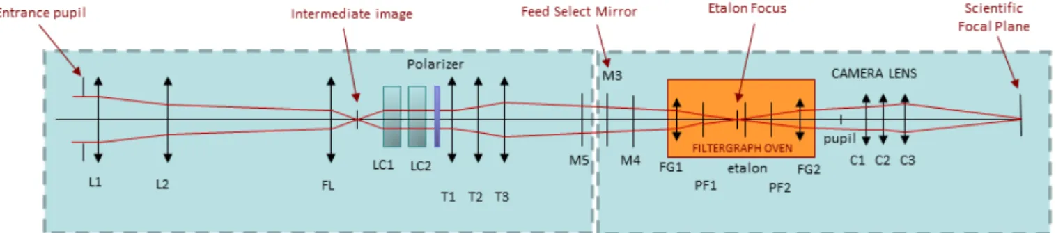
Fig. 6. Optical scheme of the HRT path and the FG (common path).
4.2. Opto-mechanical layout
4.2.1. High Resolution Telescope (HRT)
The High Resolution Telescope (HRT) has a square FOV of
0.28◦ × 0.28◦ on the sky with an angular sampling of 0.005 per
pixel (at closest perihelion; this is equivalent to 0.0015 pixel−1
for a ground-based instrument). This value corresponds to
op-timal sampling at the diffraction limit of a 140 mm aperture
tele-scope in the red. For this sampling, the effective focal length of the HRT path must be 4125 mm in the science focal plane, and 7920 mm in the etalon focus, respectively. Since this is more than 10 times the physical length of the SO/PHI instrument, the op-tical system needs two internal magnifications. The HRT there-fore consists of a two-mirror telescope, which is combined with a negative magnifying lens (Barlow lens). The stand-alone