A deeper look at the GD1 stream: density variations and wiggles

Publisher’s version / Version de l'éditeur:

Monthly Notices of the Royal Astronomical Society, 477, 2, pp. 1893-1902,

2018-03-14

READ THESE TERMS AND CONDITIONS CAREFULLY BEFORE USING THIS WEBSITE. https://nrc-publications.canada.ca/eng/copyright

Vous avez des questions? Nous pouvons vous aider. Pour communiquer directement avec un auteur, consultez la

première page de la revue dans laquelle son article a été publié afin de trouver ses coordonnées. Si vous n’arrivez pas à les repérer, communiquez avec nous à PublicationsArchive-ArchivesPublications@nrc-cnrc.gc.ca.

Questions? Contact the NRC Publications Archive team at

PublicationsArchive-ArchivesPublications@nrc-cnrc.gc.ca. If you wish to email the authors directly, please see the first page of the publication for their contact information.

Archives des publications du CNRC

This publication could be one of several versions: author’s original, accepted manuscript or the publisher’s version. / La version de cette publication peut être l’une des suivantes : la version prépublication de l’auteur, la version acceptée du manuscrit ou la version de l’éditeur.

For the publisher’s version, please access the DOI link below./ Pour consulter la version de l’éditeur, utilisez le lien DOI ci-dessous.

https://doi.org/10.1093/mnras/sty677

Access and use of this website and the material on it are subject to the Terms and Conditions set forth at

A deeper look at the GD1 stream: density variations and wiggles

De boer, T. J. L.; Belokurov, V.; Koposov, S. E.; Ferrarese, L.; Erkal, D.;

Côté, P.; Navarro, J. F.

https://publications-cnrc.canada.ca/fra/droits

L’accès à ce site Web et l’utilisation de son contenu sont assujettis aux conditions présentées dans le site LISEZ CES CONDITIONS ATTENTIVEMENT AVANT D’UTILISER CE SITE WEB.

NRC Publications Record / Notice d'Archives des publications de CNRC:

https://nrc-publications.canada.ca/eng/view/object/?id=0bb982d9-3093-445d-bc82-4fa28777dde2

https://publications-cnrc.canada.ca/fra/voir/objet/?id=0bb982d9-3093-445d-bc82-4fa28777dde2

A deeper look at the GD1 stream: density variations and wiggles

T.J.L. de Boer

, V. Belokurov

, S. E. Koposov

, L. Ferrarese

,D. Erkal

, P. Cˆot´e

and J.F. Navarro

1_{Department of Physics, University of Surrey, Guildford, GU2 7XH, UK}

2_{Institute of Astronomy, University of Cambridge, Madingley Road, Cambridge, CB3 0HA, UK} 3_{Center for Computational Astrophysics, Flatiron Institute, 162 5th Avenue, New York, NY 10010, USA}

4_{McWilliams Center for Cosmology, Department of Physics, Carnegie Mellon University, 5000 Forbes Avenue, Pittsburgh, PA 15213, USAs} 5_{National Research Council of Canada, 5071 West Saanich Road, Victoria, BC, V9E 2E7, Canada}

6_{Department of Physics and Astronomy, University of Victoria, Victoria, BC, Canada V8P 5C2}

Received ...; accepted ...

ABSTRACT

Using deep photometric data from CFHT/Megacam, we study the morphology and density of the GD-1 stream, one of the longest and coldest stellar streams in the Milky Way. Our deep data recovers the lower main sequence of the stream with unprecedented quality, clearly separating it from Milky Way foreground and background stars. An analysis of the distance to different parts of the stream shows that GD-1 lies at a heliocentric distance between 8 and 10 kpc, with only a shallow gradient across 45 deg on the sky. Matched filter maps of the stream density show clear density variations, such as deviations from a single orbital track and tentative evidence for stream fanning. We also detect a clear under-density in the middle of the stream track at ϕ1=-45 deg surrounded by overdense stream segments on either side.

This location is a promising candidate for the elusive missing progenitor of the GD-1 stream. We conclude that the GD-1 stream has clearly been disturbed by interactions with the Milky Way disk or other sub-halos.

Key words: Galaxy: structure – Galaxy: fundamental parameters — Stars: C-M diagrams — Galaxy: halo

1 INTRODUCTION

Stellar streams provide a dramatic confirmation of the hierarchical galaxy formation scenario, showing us that large galaxies accrete smaller stellar systems (Lynden-Bell & Lynden-Bell 1995). The streams are the relics of this formation process, consisting of stars stripping from the infalling host cluster or galaxy (Newberg 2016). Large scale, homogeneous sky surveys such as SDSS, 2MASS, Pan-STARRS, ATLAS, and DES (Skrutskie et al. 2006; Ahn et al. 2014; Shanks et al. 2015; Chambers et al. 2016) have been success-fully mined for stream features, resulting in nearly a dozen streams to date (Shipp et al. 2018). These streams show a wide variety of morphologies, ranging from the wide and long Sagittarius stream to the very short Ophiuchus stream (Belokurov et al. 2006; Bernard et al. 2014). The orbits of streams have been used to place some of the strongest constraints on the mass distribution of the Milky Way (MW) to date (e.g., Koposov, Rix & Hogg 2010; Law & Majewski 2010; Gibbons, Belokurov & Evans 2014; Bowden, Belokurov & Evans 2015; K¨upper et al. 2015; Bovy et al. 2016). Streams also represent one of the very few ways of probing the existence of dark matter (DM) subhalos (e.g. Ibata et al. 2002; Johnston, Spergel &

⋆ _{E-mail: t.deboer@surrey.ac.uk}

Haydn 2002; Carlberg 2009; Yoon, Johnston & Hogg 2011; Carl-berg 2012; Erkal & Belokurov 2015a), which are not expected to form any stars (Ikeuchi 1986; Rees 1986). Analysis of deep data for the Pal 5 stream has indeed shown tentative evidence of a distur-bance by low mass subhaloes (Bovy, Erkal & Sanders 2017; Erkal, Koposov & Belokurov 2017).

The GD-1 tidal stream was first discovered by Grillmair & Dionatos (2006) in the Sloan Digital Sky Survey (SDSS) as a 63 degree long trail of stars extending from the constellation of Ursa Major to Cancer. The stream is very thin on the sky (σ ≈0.2 deg), indicating that it most likely originated in a globular cluster (GC) stripping event (Koposov, Rix & Hogg 2010). GD-1 is among the most suitable streams for the study of the lumpiness of DM, satisfy-ing several necessary conditions. First, the stream has a small initial phase-space volume, facilitating a clean separation of the velocity kicks induced by dark substructures from the secular dynamics of the progenitor. Moreover, the stream is long enough to have experi-enced many possible interactions, and has a high surface brightness which allows us to measure the stream density with high accuracy (Erkal et al. 2016). This makes it easier to detect density perturba-tions along the stream.

While the theory behind stream gap formation is well devel-oped (Yoon, Johnston & Hogg 2011; Carlberg 2012; Erkal &

lokurov 2015a; Sanders, Bovy & Erkal 2016), determining whether an observed gap is the result of a dark subhalo passage is more dif-ficult. For many streams (including the Pal 5 stream) gaps may re-sults from an interaction with a giant molecular cloud (Amorisco et al. 2016) or the MW bar (Erkal, Koposov & Belokurov 2017; Pearson, Price-Whelan & Johnston 2017). However, the derived or-bits of the GD-1 stream show that it is moving in a retrograde sense with respect to the disk with a perigalacticon of about 14 kpc and apogalacticon of 26-29 kpc (Koposov, Rix & Hogg 2010; Bowden, Belokurov & Evans 2015). This would imply that interactions with disk sub-strucure are less likely, and thus make it an ideal candidate for the study of gaps induced by dark subhalos.

To date, the stellar content of the stream has not yet been stud-ied in depth, due to the relatively shallow photometric data and small numbers of spectroscopic members. Based on isochrone fit-ting of SDSS photometry, the stream is best matched to a relatively metal-rich population with [Fe/H]=-1.4 and an age of ≈9 Gyr (Ko-posov, Rix & Hogg 2010). However, based on spectroscopic mea-surements from the SDSS SEGUE survey (Yanny et al. 2009) a more metal-poor population with [Fe/H]=-1.9 and ancient age is favoured (Willett et al. 2009). The stream does not have any ap-parent progenitor, but its low spectroscopic metallicity and small angular width suggest that a GC origin is more appropriate than a dwarf galaxy. Although it is possible that the progenitor may be lo-cated outside the currently studied stream footprint, no known star cluster or galaxy has been found to match the orbital properties of the stream. It is also possible the parent satellite has by now fully dissolved, leaving no detectable remnant behind.

Studies using SDSS photometry have indicated that there may be density variations along the GD-1 stream. Analysis by Koposov, Rix & Hogg (2010) shows the presence of several under-densities of varyious sizes, which do not correlate with CCD gaps in the Sloan camera, fluctuations in dust extinction or other sources of spurious detections. More recently, Carlberg & Grillmair (2013) investigated the same SDSS data for the presence of stream gaps. A total of 8 tentative gaps are detected along the stream, albeit with limited confidence. The number of large gaps is in good agree-ment with predictions for DM sub-halo encounters with cold star streams, while the number of small gaps is well below predic-tions (Carlberg & Grillmair 2013). The mechanism responsible for these gaps is not clear, in part due to the lack of a progeni-tor (K¨upper, MacLeod & Heggie 2008; K¨upper, Lane & Heggie 2012). More recently, Erkal et al. (2016) predicted the number of gaps from subhaloes expected in GD-1 and argued that there should be no small gaps but rather roughly 1 gap with a size on the order of ∼ 6.5 degrees if GD-1 were on a circular orbit. Since GD-1 is currently close to pericenter (Koposov, Rix & Hogg 2010; Bow-den, Belokurov & Evans 2015), the gap should be larger than this on average.

In this work, we investigate the spatial distribution of GD-1 stream stars, using deep, wide-field CFHT data. This new data goes ≈2 magnitudes deeper than the shallow SDSS photometry and reaches the level of faint Main Sequence stars across a 45 degree stretch of the stream. The greater depth affords a cleaner separation of the GD-1 features from those of the Milky Way stellar halo, al-lowing us to determine more accurate distances than possible from SDSS photometry. We study the evolution of the stream centroid on the sky and search for variations such as wiggles around the mean track, which are indicative of perturbations due to tidal encounters (Carlberg 2012; Erkal & Belokurov 2015a,b). Finally, we study the stream’s density profile on large scales as well as small-scale den-sity variations with greater spatial resolution than previously

pos-sible, and look for under-densities and gaps. This provides a new, clearer view of the GD-1 stream.

This paper is organised as follows: in Section 2 we present the CFHT photometric dataset used, the data reduction procedure and discuss the resulting catalog. In Section 3 we determine the stream track and the distance to different parts of the stream. This is followed in Section 4 by matched filter maps of GD-1 and an analysis of stellar density variations. Finally, Section 5 discusses the results and their implications for the lumpiness of DM.

2 DATA

Deep optical photometry of the GD-1 stream in the g and r fil-ters was obtained using the Megacam camera on CFHT as part of observing proposals 15AC13 and 16AC03 (PI: de Boer). Observa-tions consisted of 4 dithered exposures of 50s each, in both g and r bands, under dark conditions and seeing less than 0.8 arcsec. Point-ings were overlapped and dithered to fill CCD and tiling gaps and obtain the most homogeneous spatial coverage. The images were astrometrically calibrated against SDSS and subsequently swarped to a common grid with a maximum number of 4 stacked images, to achieve a homogeneous data depth (Bertin et al. 2002). Following this, the images were reduced with the help of SExtractor and PS-Fex (Bertin & Arnouts 1996). The resulting catalogues were photo-metrically calibrated using SDSS photometry and corrected for ex-tinction using dust maps from Schlegel, Finkbeiner & Davis (1998) with coefficients from Schlafly & Finkbeiner (2011), on a star by star basis.

The spatial coverage of the deep photometry is shown in Fig-ure 1 in equatorial, Galactic and rotated-spherical heliocentric great circle coordinates aligned with the stream (Koposov, Rix & Hogg 2010). The observations resulted in a total coverage of 45 degrees along the stream and out to at least 4 times the width of the stream. No obvious signs of pointing or tiling marks are visible in the bot-tom panel of Figure 1, showing that our catalogue is flat and homo-geneous across the footprint.

Figure 2 displays the photometric error as a function of mag-nitude for each filter for all stars in the catalogue. The photo-metric error profile is narrow and well defined, showing no hints of pointings with anomalous depth. The right panels of Figure 2 show the SExtractor SPREAD MODEL parameter as function of magnitude. Our final sample of stars are selected using a cut at |SPREAD MODEL| <0.002 +SPREADERR MODEL to discriminate between likely stars and unresolved galaxies.

Figure 3 shows the (r,g−r) CMD of all stellar objects in our data following the centre of the stream coordinate frame with |ϕ2| <0.2 degrees. The bottom panel also shows the CMD of our

off-stream background region with 0.5< |ϕ2| <0.8 degrees, which

is free from stream stars. The CMDs display all typical features commonly associated with the MW foreground (including the red disk MS stars at g−r=1.5 and faint blue halo stars at g−r=0.3). However, the CMD of the stream region also displays a clear di-agonal overdense sequence of GD-1 stream stars, extending from g−r=0.3, r=19 to g−r=1.1, r=23 which corresponds to the lower MS and turn-off of the stream. This GD-1 sequence clearly stands out from the underlying MW halo contamination, and is well traced by the reference isochrone for GD-1 populations. We adopt a reference isochrone with [Fe/H]=−1.9, an age of 12 Gyr, and a distance of 9 kpc is from the Dartmouth isochrone library (Dotter et al. 2008).

The CMD shows the presence of overdense features on the blue side of the CMD with g−r≈0 fainter than the GD-1 MSTO.

Figure 1. Spatial coverage of all stars in the CFHT/Megacam photometry of the GD-1 stream, in equatorial coordinates ra,dec (top), Galactic coordi-nates l,b (middle) and in coordicoordi-nates aligned with the stream (bottom). The colour indicates the density of stars across the footprint.

Figure 2. Data quality overview showing the photometric errors as a func-tion of g and r filters in the left panels and the SPREAD MODEL parameter in the right panels. The black dashed lines in the right panels indicate the SPREAD MODEL_{selection adopted to remove unresolved galaxies from the} catalog.

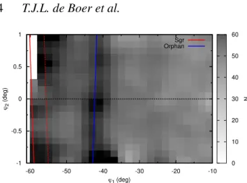
They have colours reminiscent of Blue Horizontal Branch or Blue Straggler Stars, but could also constitute a more metal-poor MS turnoff at larger distance. Therefore, we select all stars with -0.1<g-r<0.5 and 22<r<23 and show their spatial density map in Figure 4. Two clear sequences are visible in the density map, per-pendicular to the direction of the GD-1 stream. Comparison to the overlaid stream tracks shows that these features correspond to the Sgr stream and Orphan stream, both of which are further away and more metal-poor than the GD-1 stream.

3 DISTANCE AND STREAM TRACK

With calibrated data in hand, we turn to the determination of the stream parameters, such as distance and position on the sky. Due to the greater depth and increased accuracy of the CFHT data over

|ϕ2|<0.2 deg obs-Galaxia -0.2 0 0.2 0.4 0.6 0.8 1 1.2 1.4 g-r 15 16 17 18 19 20 21 22 23 24 r 0 10 20 30 40 50 60 70 N |ϕ2|<0.2 deg 0 10 20 30 40 50 60 70 N |ϕ2|<0.2 deg -0.5 0 0.5 1 1.5 g-r 14 16 18 20 22 24 r 0 10 20 30 40 50 60 70 N 0.5<|ϕ2|<0.8 deg 0 10 20 30 40 50 60 70 N

Figure 3. The colour-magnitude diagram of our data, overlaid with a refer-ence isochrone for GD-1 with parameters ([Fe/H]=−1.9, 12 Gyr) at a dis-tance of 9 kpc. The top panel shows the observed Hess diagram of all stars in the stream with |ϕ2| <0.2 degrees, while the bottom panel shows the Hess

diagram for the background using 0.5< |ϕ2| <0.8 degrees. The lower main

sequence and turn-off of the GD-1 population is clearly visible, as traced by the reference isochrone.

SDSS catalogues, we can make use of the faint MS to determine the distance to the GD-1 stream. Therefore, we select stars with main sequence colours (0.5<g-r<0.9) and magnitudes correspond-ing to dwarfs (19<r<23) and compare their magnitude to those of the GD-1 reference isochrone. For each star, we compute the dif-ference between its r-band magnitude and the magnitude expected for the isochrone. These differences are then summed up to create a distance modulus histogram for each bin of ϕ1considered.

To bring out the signal of the GD-1 stream, we correct for the effects of MW contamination using the Galaxia model of the MW (Sharma et al. 2011). A Galaxia realisation is generated in small bins of Galactic longitude and latitude along the stream foot-print and convolved with the photometric scatter due to magnitude dependent errors shown in Figure 2. We then compute the same dis-tance modulus offsets for the Galaxia realisation as for the observed CMD and subtract it from the on-stream results.

Figure 5 displays the MS distance modulus for the GD-1 stream, as determined for our stellar sample after MW correction. A clear sequence is visible, for distance modulus of ≈14.7 or ≈9 kpc. To determine the heliocentric distance at each position in the stream, we fit a Gaussian to the density histogram in each ϕ1along

-60 -50 -40 -30 -20 -10 ϕ1 (deg) -1 -0.5 0 0.5 1 ϕ2 (deg) 0 10 20 30 40 50 60 N Sgr Orphan

Figure 4. The spatial density of faint, blue stars (-0.1<g-r<0.5 and 22<r<23) across the GD-1 footprint. Lines indicate the trajectory of known streams in this part of the sky, such as the Sagittarius bright stream (red lines) and the Orphan stream in blue (Belokurov et al. 2007; Koposov et al. 2012).

with a second order polynomial background and determine the cen-tre and standard deviation. The red line in Figure 5 indicates the determined distance to GD-1, while the blue line indicates the re-sults from Koposov, Rix & Hogg (2010). Values for the Gaussian centre and standard deviation are also given (along with their uncer-tainties) in Table 1. Finally, the green (dotted) line shows a second order polynomial fit to the distances, as described by the function f(ϕ1)=14.58 +(2.923e-4*(ϕ1+44.66)2). This function will be

subse-quently used to correct for the distance to GD-1. Figure 5 indicates that GD-1 shows a gradually increasing distance as ϕ1 increases,

ranging from ≈8 to 10 kpc. Compared to the results of Koposov, Rix & Hogg (2010), our data indicate the stream is on average slightly more distant but in good agreement at higher ϕ1. Our new

results show less variation in the distance to GD-1 in this part of its footprint, with a change of only 1.5 kpc over 45 degrees. The derived results correspond to a range in galactocentric distances between 13 and 15 kpc, which is consistent with the perigalacticon distance of best-fit GD1 orbits (Carlberg & Grillmair 2013).

With the distance to the stream in place, we next determine the track of the stream on the sky. To determine the stream track, we first perform a matched filtering of the data, assuming that the GD-1’s CMD is well described by an isochrone with [Fe/H]=−1.9, 12 Gyr and distances from Table 1. Similar to Erkal, Koposov & Belokurov (2017), we forgo using a classical matched filter tech-nique (in which weighted data is no longer Poisson distributed) and instead adopt a boolean mask procedure. For the signal mask we populate the [Fe/H]=−1.4, 9 Gyr isochrone using a Kroupa IMF (Kroupa 2001) and convolve the synthetic stars with the photo-metric errors as function of magnitude extracted from the observed data. To avoid a filter that is arbitrarily thin at bright magnitudes (where photometric errors are small), a minimum filter width of 0.05 is adopted. For the background filter, we generate an oversam-pled Galaxia MW model for each pixel (to ensure enough stars pop-ulate the CMD) and once again convolve stars with the observed photometric errors. Both masks are normalised, and the fraction Pstr(g-r,r)/Pbg(g-r,r) is used to select CMD pixels below a certain

threshold. For each pixel, the threshold value is chosen by looping through the possible values and finding the one which maximises the signal-to-noise. We then assign a weight of zero to values of Pstr(g-r,r)/Pbg(g-r,r) lower than the threshold and a weight of 1 for

value higher than the threshold.

-55 -50 -45 -40 -35 -30 -25 -20 -15 -10 ϕ1 (deg) 13 13.5 14 14.5 15 15.5 16 m-M (mag) 0 10 20 30 40 50 N obs-Galaxia Koposov 2010 this work

Figure 5. MS distance modulus as a function of ϕ1for the GD-1 stream.

The figure shows the density of stars in magnitudes offset from the MS between 0.5<g-r<0.9 and r>19, after MW correction. The red line indicates the location of the best Gaussian fit to each bin of ϕ1, while the blue line

indicates the distance determination from (Koposov, Rix & Hogg 2010). The green (dotted) line shows a best fit second order polynomial to the distances, described by the function f(ϕ1)=14.58 +(2.923e-4*(ϕ1+44.66)2).

Table 1. Distance modulus and heliocentric distance to the GD-1 stream for bins of ϕ1position.

ϕ1 m-M σm−M distance σdistance (deg) (mag) (mag) (kpc) (kpc) -52.5 14.56±0.01 0.12±0.01 8.15±0.04 0.45±0.01 -47.5 14.60±0.04 0.11±0.04 8.32±0.15 0.42±0.14 -42.5 14.57±0.05 0.09±0.05 8.21±0.19 0.34±0.18 -37.5 14.64±0.09 0.20±0.01 8.46±0.35 0.78±0.03 -32.5 14.72±0.05 0.14±0.06 8.78±0.20 0.57±0.22 -27.5 14.64±0.06 0.20±0.01 8.46±0.23 0.78±0.03 -22.5 14.67±0.10 0.20±0.11 8.57±0.40 0.79±0.43 -17.5 14.87±0.07 0.10±0.07 9.40±0.30 0.42±0.31 -12.5 14.92±0.04 0.10±0.04 9.63±0.18 0.44±0.17

From the analysis of the CMD in Figure 3 we have shown signs of the Orphan stream population in our data, partially overlap-ping with the main sequence of GD-1. The density of Orphan stars intersecting the GD1 main sequence is low, given its much greater distance. Nonetheless, given the position of the Orphan stream in our footprint (see Figure 4), contamination might influence the GD-1 stream track at low ϕ1. Therefore, we include an extra background

filter during the matched filter process, based on the Orphan stream stellar populations and distance. This ensures that CMD bin coinci-dent with the Orphan stream stellar population locus are penalised in the filtering, thereby avoiding Orphan stream contamination.

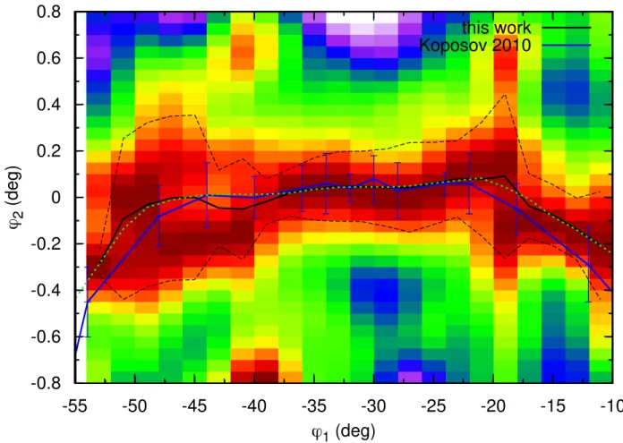
Figure 6 shows the matched filter map of GD-1 using rough spatial bins of 2×0.05 deg. To bring out low contrast stream fea-tures in more detail, the map is convolved using a Gaussian kernel of 2×0.05 deg, and normalised in each ϕ1column. A clear sequence

is visible around ϕ2 ≈0 deg, which corresponds to the track of

the GD-1 stream. For reference, the stream track of GD-1 derived in Koposov, Rix & Hogg (2010) is overlaid as the blue line with errorbars. The track of GD-1 extracted here is roughly consistent with the Koposov, Rix & Hogg (2010) track, showing a distinct

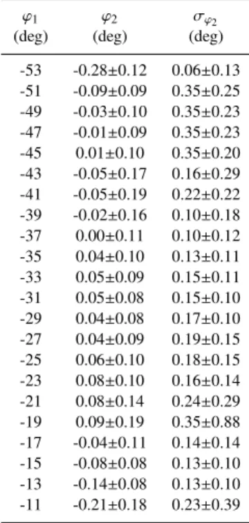
Table 2. Position and width of the GD-1 stream, as shown in Figure 6.

ϕ1 ϕ2 σϕ2

(deg) (deg) (deg) -53 -0.28±0.12 0.06±0.13 -51 -0.09±0.09 0.35±0.25 -49 -0.03±0.10 0.35±0.23 -47 -0.01±0.09 0.35±0.23 -45 0.01±0.10 0.35±0.20 -43 -0.05±0.17 0.16±0.29 -41 -0.05±0.19 0.22±0.22 -39 -0.02±0.16 0.10±0.18 -37 0.00±0.11 0.10±0.12 -35 0.04±0.10 0.13±0.11 -33 0.05±0.09 0.15±0.11 -31 0.05±0.08 0.15±0.10 -29 0.04±0.08 0.17±0.10 -27 0.04±0.09 0.19±0.15 -25 0.06±0.10 0.18±0.15 -23 0.08±0.10 0.16±0.14 -21 0.08±0.14 0.24±0.29 -19 0.09±0.19 0.35±0.88 -17 -0.04±0.11 0.14±0.14 -15 -0.08±0.08 0.13±0.10 -13 -0.14±0.08 0.13±0.10 -11 -0.21±0.18 0.23±0.39

down-turn at both sides of our footprint. However, there are also deviations from the track, particularly on the left side, which corre-sponds to low Galactic latitude. To fit the GD-1 stream track in our new data, we fit a Gaussian model and background to each column of ϕ1. The recovered stream track is shown as the solid black line

in Figure 6, with the width indicated by dashed lines. The values for the track centre and width are also listed in Table 2. Figure 6 shows the GD-1 stream is very narrow in the middle -40< ϕ1<-25

deg stretch, with a total width of ≈0.3 deg. At low ϕ1 values, the

stream becomes much broader and appears to show some wiggles. The stream track is not smooth and shows some wiggles due to uncertainties in the track determination, which could introduce artificial wiggles in the stream density around the track. Therefore, we smooth the track using a simple boxcar filter, resulting in the green dotted line in Figure 6. This smooth track will subsequently be used to determine the density and variation of the GD-1 stream. To check the validity of the track and distance determination, we extract the CMD of GD-1 stars around the stream track, and correct for the distance variation, shifting stars to a common dis-tance modulus of m-M=14.50. The g−r,r CMD after subtracting the Galaxia MW model realisation is shown in Figure 7, along with the GD-1 reference isochrone overlaid. The GD-1 main sequence and turn-off are both clearly visible, along with the start of the sub-giant branch. The GD-1 main sequence appears much sharper in the corrected CMD, compared to Figure 3, indicating a good distance correction. The narrow width of the main sequence is obvious, rul-ing out a composite stellar population. This shows once again the GD-1 stream was likely formed from the stripping of a GC, instead of a dwarf galaxy.

4 GD-1 STREAM DENSITY

With the distance and stream track determined, we can now start constructing density maps of the GD-1 stream with greater

resolu-tion. Similar to Section 3, we once again perform a matched filter mapping of the data. However, this time, we offset the data in ϕ2

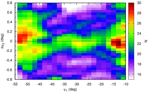
using the stream track positions of Table 2 to be able to see vari-ations and wiggles of GD-1 around the track. The maps are con-structed using spatial bins of 2×0.1 deg to reveal the stream density in greater detail. Figure 8 shows the matched filter map of the GD-1 stream, before (top panel) and after (bottom panel) column normal-isation. In the top panel of Figure 8, we show the resulting matched filter density map of the GD-1 stream. To bring out the shape of the GD-1 stream track, we also show a column normalised version of the map in the bottom panel. This map is constructed by indi-vidually normalising the stream density in each column of ϕ1. A

column normalised map is often used to bring out connected low density features in the presence of varying background contamina-tion, and will highlight the region of high density at each ϕ1.

As expected, the stream density largely follows the stream track determined in Section 3, with density peaking around ϕ2=0.

There are however strong density variations as function of ϕ1, with

an obvious lower density area around ϕ1≈-40 deg, and higher

den-sity regions at either end of our footprint. The column normalised map in Figure 8 shows that GD-1 displays clear wiggles around the stream track. Apart from the large deviation at ϕ1=-45 deg, the

stream shows wiggles offset from the track by an amount smaller than its width of ≈0.1 deg.

The normalised density map in the botton panel of Figure 8 shows that the stream is thin for ϕ1>-40 deg, with a wider section

around ϕ1=-20 deg. On the left side of the footprint, the stream is

much wider and shows clear deviations from the stream track. Most strikingly, at ϕ1=-45 deg we see an underdensity centered around

ϕ2=0 with overdense segment at both higher and lower ϕ2. The two

stream segments appear to wrap around the central under density, giving the appearance of tidal tails coming off a completely de-stroyed progenitor. However, we are not claiming to have found the progenitor, but merely commenting on the appearance of this striking feature. We note that perturbations from subhaloes can also produce similar oscillations in the stream track (Erkal & Belokurov 2015a). The central depletion is clearly visible in the top panel of Figure 8, and consists of an ≈20% drop in stream density. A larger coverage of the GD-1 stream on the low ϕ1side is needed to

unam-biguously determine the nature of this feature.

The density of the GD-1 stream can be studied in more detail by constructing density histogram along and perpendicular to the stream track. To correct for the presence of foreground and back-ground contaminants, we construct a model of contaminant sources by fitting a polynomial function to the matched filter densities in the offstream region (0.6< |ϕ2| <1.0) where the contaminants

dom-inate. We adopt a second order polynomial in ϕ1and first order in

ϕ2to allow for large scale variation as function of Galactic latitude

(which lines up largely with ϕ1) while the limited coverage of ϕ2

only allows a straight line fit.

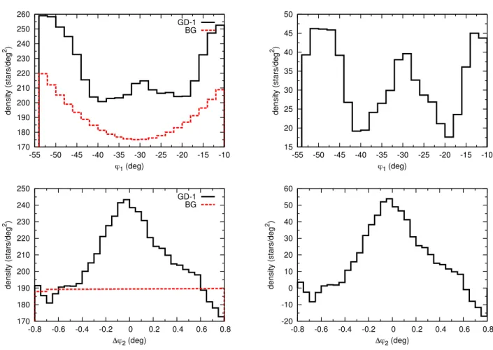
Figure 9 shows the 1D density histograms of GD-1 stars, as function of ϕ1(top) and ϕ2(bottom). The left panels show the

den-sity as obtained in Figure 8, while the right panels show the denden-sity after correcting for contamination from the Milky Way. The den-sity as function of ϕ2clearly peaks around zero and falls off rapidly

to background levels. At positive ϕ2, the density is higher than on

the negative side, which appears to be due to residual patches of contamination at ϕ2=0.5. The density can be fit using a Gaussian

profile with a width of 0.16 deg, showing that the GD-1 stream is very narrow across the studied 45 degrees.

The background corrected stream density in Figure 9 shows GD-1 has a density of ≈40 stars/deg2_{across our range of studied ϕ}

-55

-50

-45

-40

-35

-30

-25

-20

-15

-10

ϕ

₁

(deg)

-0.8

-0.6

-0.4

-0.2

0

0.2

0.4

0.6

0.8

ϕ

2

(deg)

this work

Koposov 2010

Figure 6. Matched filter map of the GD-1 stream using spatial bins of 2×0.05 deg. The map has been normalised in each ϕ1column. The black solid and

dashed lines indicate the best-fit Gaussian location and standard deviation of the stream track at each ϕ1position. The blue line and error bars indicate the

stream positions from Koposov, Rix & Hogg (2010). Finally, the green line shows the smoothed track after applying a boxcar filter.

0 0.2 0.4 0.6 0.8 1 1.2 1.4 g-r 15 16 17 18 19 20 21 22 23 24 r 0 20 40 60 80 100 N GD-1 streams obs-Galaxia

Figure 7. The colour-magnitude diagram of the GD-1 stream, extracted around the stream track determined from Figure 6 and corrected for dis-tance variations. A reference isochrone for GD-1 is overlaid with parame-ters ([Fe/H]=−1.9, 12 Gyr). The top panel shows the observed Hess diagram of all stars, while the bottom panel shows the Hess diagram after correct-ing for MW contamination uscorrect-ing the Galaxia model of the MW (Sharma et al. 2011). The lower main sequence and turn-off of the GD-1 population is clearly visible, as traced by the reference isochrone.

punctuated by two large under densities at ϕ1=-40 and ϕ1=-20 deg.

These two density drops are significant and clearly visible in the 2D spatial density maps of Figure 8. The dip at ϕ1=-20 deg corresponds

to a disturbance in Figure 8 where the stream fans out and appears discontinuous. This could be an indication of tidal effects due to a close MW passage or a flyby of a subhalo. Given the distance and orbit of GD-1, an interaction with a giant molecular cloud is unlikely (Amorisco et al. 2016). The under-density at ϕ1=-40 deg is

wider and deeper and seems linked to the central density depletion at ϕ1 ≈-45 deg. The two features are not entirely coincident in the

2D and 1D maps due to the added density of the outlying wiggles at ϕ1=-45 deg. Interestingly, the presence of underdensities along with

stream track variations in a generic prediction of the signature that subhalo perturbations produce in a stream (Carlberg 2012; Erkal & Belokurov 2015a,b). However, additional modelling is needed to determine if these features are due to an external perturbation or the secular disruption of a progenitor.

The density of foreground and background sources (in red) shows a higher value at either end of our footprint. Figure 1 shows that the left part of our footprint corresponds to the lowest Galactic latitudes. Qualitatively, the behaviour of the contaminants could be due to an increasing number of MW halo stars for higher ϕ1(i.e.

greater Galactic latitude), and an increasing number of thick and thin disk stars at the low latitude end of our footprint. While the density of thin and thick stars is typically much higher than that

-55

-50

-45

-40

-35

-30

-25

-20

-15

-10

ϕ

(deg)

-0.8

-0.6

-0.4

-0.2

0

0.2

0.4

0.6

0.8

∆

ϕ

(deg)

16

18

20

22

24

26

28

30

N

-55

-50

-45

-40

-35

-30

-25

-20

-15

-10

ϕ

(deg)

-0.8

-0.6

-0.4

-0.2

0

0.2

0.4

0.6

0.8

∆

ϕ

(deg)

0.6

0.65

0.7

0.75

0.8

0.85

0.9

0.95

1

N

Figure 8. Matched filter map of the GD-1 stream after stream track correction, using spatial bins of 2×0.1 deg bins. The top panel shows a convolved matched filter density map, while the bottom panel shows a column normalised map to increase the stream track contrast. The maps have been convolved using a Gaussian kernel of 2×0.1 deg.

170 180 190 200 210 220 230 240 250 -0.8 -0.6 -0.4 -0.2 0 0.2 0.4 0.6 0.8 density (stars/deg 2 ) ∆ϕ2 (deg) GD-1 BG 170 180 190 200 210 220 230 240 250 260 -55 -50 -45 -40 -35 -30 -25 -20 -15 -10 density (stars/deg 2 ) ϕ1 (deg) GD-1 BG -20 -10 0 10 20 30 40 50 60 -0.8 -0.6 -0.4 -0.2 0 0.2 0.4 0.6 0.8 density (stars/deg 2) ∆ϕ2 (deg) 15 20 25 30 35 40 45 50 -55 -50 -45 -40 -35 -30 -25 -20 -15 -10 density (stars/deg 2 ) ϕ1 (deg)

Figure 9. Density histograms of GD-1 stars in the matched filter map after stream track correction, as function of ϕ1(top) and ϕ2(bottom). The left panels

show the density of the regular and convolved maps along with the density of background sources as fit from the offstream region. The right panels show the density after subtracting the background counts.

of the halo, our matched filter preferably leads to halo contamina-tion, which may lead to a greater importance of the halo contribu-tion. However, given the importance of the background model for stream density fluctuations, and the small spatial area used to com-pute the background density, we use data from the SDSS to check its validity.

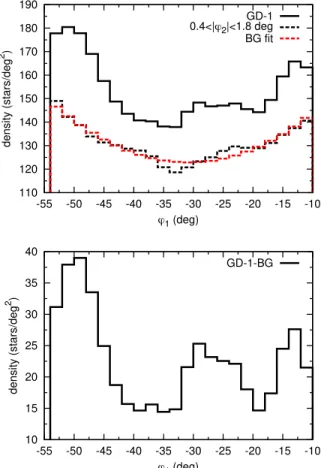
We filter the SDSS data using the exact same procedure and parameters as used to produce Figure 9 and determine the density of contamination across a much wider area of ϕ2. The top panel

of Figure 10 shows that the distribution of contaminant sources is remarkably similar in SDSS, along with the over-density of con-taminants on either end of the footprint. Therefore, we can rule out effects due to peculiarities of our data from the MW decontami-nation. Furthermore, the stream density of SDSS sources displays similar under-densities as in our deeper data, albeit with reduced contrast. This gives greater confidence to the validity of our density perturbations.

5 CONCLUSIONS AND DISCUSSION

In this work, we have utilised deep photometric CFHT data to study the distance, morphology and density of stars in the GD-1 stream. Our deep CMDs of the stream region (see Figure 7) show that the data recovers the lower main sequence of the GD-1 stream with unprecedented quality. The photometric error and spatial density

distribution (see Figures 2 and 1) show that our data sample is ho-mogeneous without obvious depth issues, essential for tracing den-sity variations across the footprint.

The GD-1 stream easily shows up in our CMDs (Figure 3) as a thin main sequence which clearly separates from the MW halo stars due to the data quality. The narrow width of the faint main sequence feature rules out a composite stellar population in GD-1, further indicating that the stream was likely formed from the stripping of a GC, instead of a dwarf galaxy.

Similar to the analysis of Koposov, Rix & Hogg (2010), we use the data to determine the distance to different parts of the stream in Section 3. We find the stream occupies a distance between 8 and 10 kpc in our studied footprint, in good agreement but slightly farther away than Koposov, Rix & Hogg (2010) results.

The distance determination makes use of the lower main sequence, thus avoiding degeneracies between distance and age/metallicity. Nonetheless, the lower main sequence in sensitive to binary stars, and a larger binary fraction for GD-1 might there-fore induce a distance bias. We have also determined the best-fit stream track by making use of a matched filter approach, following the technique described in Erkal, Koposov & Belokurov (2017). The recovered stream track is in agreement with previous results within the uncertainties but tracers the stream density in more de-tail. The stream track in Figure 6 displays some variation on small scales, which could give to rise to artificial wiggles in the track cor-rected densities. Therefore, we produce a smoothed track using a

10 15 20 25 30 35 40 -55 -50 -45 -40 -35 -30 -25 -20 -15 -10 density (stars/deg 2) ϕ1 (deg) GD-1-BG 110 120 130 140 150 160 170 180 190 -55 -50 -45 -40 -35 -30 -25 -20 -15 -10 density (stars/deg 2 ) ϕ1 (deg) GD-1 0.4<|ϕ2|<1.8 deg BG fit

Figure 10. Top: Histograms showing the density of GD-1 stars in SDSS after stream track correction, as function of ϕ1for the stream track

selec-tion (solid black line), the outer regions satisfying 0.4< ϕ2<1.8 deg (dashed

black line) and the 2D background counts fit. Bottom: The density of GD-1 stars in SDSS as function of ϕ1after subtracting the best-fit background

model. -50 -45 -40 -35 -30 -25 -20 -15 -10 ϕ1 (deg) -0.8 -0.6 -0.4 -0.2 0 0.2 0.4 0.6 0.8 ∆ ϕ2 (deg) 0.6 0.65 0.7 0.75 0.8 0.85 0.9 0.95 1 N

Figure 11. Matched filter map of the GD-1 stream from SDSS data, after stream track correction. The same distances, track offsets and CMD selec-tion as in Figure 8 are adopted.

1 0 1 2 (d eg ) 8 9 10 Dist (kpc) 200 0 200 vr (k m/ s) 60 50 40 30 20 10 1 (deg) 10 0 PM (mas/yr)

Figure 12. Simulation of a GD1-like system dissolving in a realistic MW potential. In this simulation, the progenitor is placed at ϕ1=-45 deg at the

present to assess the stream track variations resulting from a dissolving pro-genitor. Different panels show the simulated stream particles in compar-ison to our stream track (top panel) and distance results (second panel) as well literature radial velocity (third panel) and proper motion measurements (fourth panel) (Koposov, Rix & Hogg 2010). Note that in the bottom panel the blue points correspond to µφ1cos φ2while the orange points correspond

to µφ2.

simple boxcar filter, which is devoid of small scale wiggles. Given the importance of a robust stream track, performing an orbit fitting to stream would result in a smoother and more physically meaning-ful track. We plan to conduct a meaning-full non-parametric fit to the stream data in a forthcoming paper.

The stream track corrected matched filter maps of Figure 8 show clear density variations across the 45 deg of GD-1 mapped using CFHT/Megacam. Column normalised maps also show sev-eral clear deviations from the track and fanning out of the stream, indicating that GD-1 may have suffered disturbances due to interac-tions with the MW or other sub-halos. Comparison of the density variations to results from realistic GD-1 simulations in the pres-ence of flybys will be conducted in forthcoming work. Most no-tably, a clear under-density is seen in the middle of the stream track at ϕ1=-45 deg surrounded by overdense stream segments on either

side. This location is a promising candidate for the illusive missing progenitor of the GD-1 stream, for further photometric or spec-troscopic follow-up. To test for the effects of peculiarities in our survey data, we determine a matched filter map of shallower SDSS data using the same set-up as Figure 8. The column normalised map in Figure 11 displays similar features, including the central under-density at ϕ1=-45 deg. This rules out the possibility of weather,

depth variation or tiling strategy being responsible for the observed features discussed in Section 4.

Projected 1D density histograms (see Figure 9) show two large densities, one of which is located close to central under-density at ϕ1=-45 deg, while the other large dip coincides with a

clear stream fanning feature at ϕ1=-20 deg. To produce MW

decon-taminated density histograms, obtaining a robust model of the fore-ground and backfore-ground sources is crucial to constrain the under-lying stream density. In this work, we have utilised the off-stream region at 0.6< |ϕ2| <1.0 to determine the contaminant density and

its variation across ϕ1. The overall shape of the contaminant source

Fig 10), ruling out effects due to weather, depth or observational biases on the contaminant density. Nonetheless, obtaining a wider sampling around GD-1 would be recommended when determining the significance of the detected under-densities.

To assess whether the extent of stream variations and wiggles is indicative of stream disturbance, we have conducted a numerical simulation of a GD1-like system disrupting in a realistic MW po-tential. The simulation is done with the modified Lagrange Cloud stripping approach of Gibbons, Belokurov & Evans (2014) to allow us to rapidly sample many progenitor disruptions and get a best fit to the data. The progenitor is modeled as a Plummer sphere with a mass of 104_M

⊙and a scale radius of 5 pc (which gives roughly the

correct stream width on the sky) and is evolved in a realistic Milky Way potential, MWPotential2014, from Bovy (2015). The pro-genitor is placed at ϕ1=-45 deg at the present day and then rewound

for 3 Gyr, after which it is evolved to the present while tidally dis-rupting. Figure 12 shows the simulated stream particles in compar-ison to our stream track and distance results as well literature radial velocity and proper motion measurements (Koposov, Rix & Hogg 2010). Note that we simulated approximately 100 disruptions with varying proper motions to get this particular realization of GD01.

The simulated stream particles provide a good fit to the ob-served properties of GD-1 in both distance and kinematics param-eter space. The spatial distribution of the stream displays a large wiggle at ϕ1=-45 deg, the location of the progenitor. The

qualita-tive shape of the kink in the stream near the simulated progenitor is quite robust since stars are ejected from the inner and outer La-grange points (e.g. K¨upper, MacLeod & Heggie 2008) so the kink is aligned with the on-sky projection of the radial direction from the Galactic center to the stream. Since the shape of this kink is opposite to the shape seen in the data (see Fig. 8), we tentatively conclude that this wiggle is unlikely to be due to a progenitor. Furthermore, beyond the progenitor location the simulated stream track is smooth and continuous, without clear wiggles or gaps of the size as seen in Figure 8. Given the clear presence of track devi-ations in Figure 8 and density varidevi-ations in Figure 5, we therefore conclude that the GD-1 stream may have been disturbed by interac-tions with the Milky Way disk or other sub-halos. To infer the origin of the wiggles and density depletions, a more detailed comparison with numerical simulations including realistic stream disturbances is needed.

Given the proximity of the GD-1 stream at 10 kpc, stars on the upper main sequence and turn-off will be present in the second data release of the Gaia satellite (Gaia Collaboration et al. 2016), which will lead to a much better selection of stream members. The accurate proper motions from Gaia complemented by the all-sky spectroscopy from WEAVE and DESI will shed new light on the origin of density variations and the location of the missing GD-1 progenitor.

ACKNOWLEDGEMENTS

The authors have enjoyed many a conversation with the members of the Cambridge Streams Club. T.d.B. acknowledges support from the European Research Council (ERC StG-335936)

Based on observations obtained at the Canada-France-Hawaii Telescope (CFHT) which is operated by the National Research Council of Canada, the Institut National des Sciences de l’Univers of the Centre National de la Recherche Scientifique of France, and the University of Hawaii.

Funding for SDSS-III has been provided by the Alfred P.

Sloan Foundation, the Participating Institutions, the National ence Foundation, and the U.S. Department of Energy Office of Sci-ence. The SDSS-III web site is http://www.sdss3.org/.

SDSS-III is managed by the Astrophysical Research Consor-tium for the Participating Institutions of the SDSS-III Collabora-tion including the University of Arizona, the Brazilian ParticipaCollabora-tion Group, Brookhaven National Laboratory, Carnegie Mellon Univer-sity, University of Florida, the French Participation Group, the Ger-man Participation Group, Harvard University, the Instituto de As-trofisica de Canarias, the Michigan State/Notre Dame/JINA Par-ticipation Group, Johns Hopkins University, Lawrence Berkeley National Laboratory, Max Planck Institute for Astrophysics, Max Planck Institute for Extraterrestrial Physics, New Mexico State University, New York University, Ohio State University, Pennsyl-vania State University, University of Portsmouth, Princeton versity, the Spanish Participation Group, University of Tokyo, versity of Utah, Vanderbilt University, University of Virginia, Uni-versity of Washington, and Yale UniUni-versity.

REFERENCES

Ahn C. P. et al., 2014, ApJS, 211, 17

Amorisco N. C., G´omez F. A., Vegetti S., White S. D. M., 2016, MNRAS, 463, L17

Belokurov V. et al., 2007, ApJ, 658, 337 Belokurov V. et al., 2006, ApJ, 642, L137 Bernard E. J. et al., 2014, MNRAS, 443, L84 Bertin E., Arnouts S., 1996, A&AS, 117, 393

Bertin E., Mellier Y., Radovich M., Missonnier G., Didelon P., Morin B., 2002, in Astronomical Society of the Pacific Confer-ence Series, Vol. 281, Astronomical Data Analysis Software and Systems XI, Bohlender D. A., Durand D., Handley T. H., eds., p. 228

Bovy J., 2015, ApJS, 216, 29

Bovy J., Bahmanyar A., Fritz T. K., Kallivayalil N., 2016, ApJ, 833, 31

Bovy J., Erkal D., Sanders J. L., 2017, MNRAS, 466, 628 Bowden A., Belokurov V., Evans N. W., 2015, MNRAS, 449,

1391

Carlberg R. G., 2009, ApJ, 705, L223 Carlberg R. G., 2012, ApJ, 748, 20

Carlberg R. G., Grillmair C. J., 2013, ApJ, 768, 171 Chambers K. C. et al., 2016, ArXiv e-prints

Dotter A., Chaboyer B., Jevremovi´c D., Kostov V., Baron E., Fer-guson J. W., 2008, ApJS, 178, 89

Erkal D., Belokurov V., 2015a, MNRAS, 450, 1136 Erkal D., Belokurov V., 2015b, MNRAS, 454, 3542

Erkal D., Belokurov V., Bovy J., Sanders J. L., 2016, MNRAS, 463, 102

Erkal D., Koposov S. E., Belokurov V., 2017, MNRAS, 470, 60 Gaia Collaboration et al., 2016, A&A, 595, A2

Gibbons S. L. J., Belokurov V., Evans N. W., 2014, ArXiv e-prints Grillmair C. J., Dionatos O., 2006, ApJ, 643, L17

Ibata R. A., Lewis G. F., Irwin M. J., Quinn T., 2002, MNRAS, 332, 915

Ikeuchi S., 1986, Ap&SS, 118, 509

Johnston K. V., Spergel D. N., Haydn C., 2002, ApJ, 570, 656 Koposov S. E. et al., 2012, ApJ, 750, 80

Koposov S. E., Rix H.-W., Hogg D. W., 2010, ApJ, 712, 260 Kroupa P., 2001, MNRAS, 322, 231

K¨upper A. H. W., Balbinot E., Bonaca A., Johnston K. V., Hogg D. W., Kroupa P., Santiago B. X., 2015, ApJ, 803, 80

K¨upper A. H. W., Lane R. R., Heggie D. C., 2012, MNRAS, 420, 2700

K¨upper A. H. W., MacLeod A., Heggie D. C., 2008, MNRAS, 387, 1248

Law D. R., Majewski S. R., 2010, ApJ, 714, 229

Lynden-Bell D., Lynden-Bell R. M., 1995, MNRAS, 275, 429 Newberg H. J., 2016, in Astrophysics and Space Science Library,

Vol. 420, Tidal Streams in the Local Group and Beyond, New-berg H. J., Carlin J. L., eds., p. 1

Pearson S., Price-Whelan A. M., Johnston K. V., 2017, Nature Astronomy, 1, 633

Rees M. J., 1986, MNRAS, 218, 25P

Sanders J. L., Bovy J., Erkal D., 2016, MNRAS, 457, 3817 Schlafly E. F., Finkbeiner D. P., 2011, ApJ, 737, 103

Schlegel D. J., Finkbeiner D. P., Davis M., 1998, ApJ, 500, 525 Shanks T. et al., 2015, MNRAS, 451, 4238

Sharma S., Bland-Hawthorn J., Johnston K. V., Binney J., 2011, ApJ, 730, 3

Shipp N. et al., 2018, ArXiv e-prints Skrutskie M. F. et al., 2006, AJ, 131, 1163

Willett B. A., Newberg H. J., Zhang H., Yanny B., Beers T. C., 2009, ApJ, 697, 207

Yanny B. et al., 2009, AJ, 137, 4377