HAL Id: hal-02073600
https://hal.archives-ouvertes.fr/hal-02073600
Submitted on 20 Mar 2019
HAL is a multi-disciplinary open access archive for the deposit and dissemination of sci-entific research documents, whether they are pub-lished or not. The documents may come from teaching and research institutions in France or abroad, or from public or private research centers.
L’archive ouverte pluridisciplinaire HAL, est destinée au dépôt et à la diffusion de documents scientifiques de niveau recherche, publiés ou non, émanant des établissements d’enseignement et de recherche français ou étrangers, des laboratoires publics ou privés.
Approximation algorithm for scheduling applications on
hybrid multi-core machines with communications delays
Massinissa Aba, Lilia Zaourar, Alix Munier-Kordon
To cite this version:
Massinissa Aba, Lilia Zaourar, Alix Munier-Kordon. Approximation algorithm for scheduling appli-cations on hybrid multi-core machines with communiappli-cations delays. IPDPS Workshops 2018, 2018 IEEE International Parallel and Distributed Processing Symposium Workshops, May 2018, Vancouver, Canada. pp.36-45, �10.1109/IPDPSW.2018.00016�. �hal-02073600�
Approximation algorithm for scheduling applications on hybrid multi-core machines
with communications delays
Massinissa Ait Aba, Lilia Zaourar
CEA, LIST, Computing and Design Environment Laboratory
91191 GIF SUR YVETTE CEDEX, FRANCE.
Emails:{massinissa.aitaba, lilia.zaourar}@cea.fr
Alix Munier
LIP6-UPMC, 4 place Jussieu, 75005 Paris, France. Email:[email protected]
Abstract—This paper presents an efficient algorithm with performance guarantee (approximation algorithm) to solve task scheduling problem on hybrid platform. The underlying platform architecture in this work is composed by two types of resources CPU and GPU, often called hybrid parallel multi-core platforms. We consider here for each type of resource identical nodes with communications delays. We focus in finding a generic approach to schedule applications presented by DAG (Directed Acyclic Graph) that minimizes makespan by considering communication delay between processors and tasks. A 6-approximation scheduling algorithm is proposed and evaluated in comparison to exact solutions and to another method. We demonstrate that the proposed algorithm achieves a close-to-optimal performance. Finally, our algorithm has been experimented on a large number of instances. These tests assess the good practical behavior of the algorithms with respect to the state-of-the-art solutions whenever these exist. Index Terms—DAG applications, makespan, hybrid CPU GPU, approximation algorithm, scheduling.
1. Introduction
The past few years have seen an increase demand for developing efficient large computational resources. Thus, heterogeneous computing systems become a popular and powerful commercial platform, containing several heteroge-neous processing elements such as Central Processing Unit (CPU), Graphics Processing Unit (GPU) and some Field Programmable Array (FPGA) with different computational characteristics. In particular, the number of platforms of the TOP500 [1] equipped with accelerators has significantly increased during the last years. However, using efficiently these platforms became very complicated. Consequently, more and more attention has been focused on scheduling techniques for solving the problem of optimizing the exe-cution of parallel applications on heterogeneous computing systems [4], [18], [25].
The underlying platform architecture in this work is composed by two types of resources CPU and GPU often
called hybrid parallel multi-core platforms. We consider here for each type of resource identical nodes. In several appli-cations, we always observe an acceleration of the execution time of tasks if they are executed on a GPU compared to their execution time on a CPU [8]. However, we consider here the more general case where the relation between the two resources can differ for different tasks. Thus we have to take into account that the execution time for any task of the application depends on the type of resource used to execute it. This configuration is known as ”inconsistent heterogeneity” and has been well-studied in the literature. The consistent model problem was presented in [3] for the particular case of applications represented by chain of tasks, where the execution time of the task depends on the frequency of the processor to which it is assigned.
We focus here in finding a generic approach to schedule applications presented by DAG (Directed Acyclic Graph) that minimizes finish time of the application by consider-ing communication delay between processors and tasks. 6-approximation scheduling algorithm is proposed and evalu-ated compared to exact solution and to another method. We demonstrate that the proposed algorithm achieves a close-to-optimal performance. The goal here is to minimize the finish execution time of the last task of the application (usually called makespan).
The rest of the paper is organized as follow: Section 2 investigates previous research in scheduling strategies to minimize makespan on hybrid platforms. Section 3 presents the detailed problem with mathematical formulation. In Sec-tion 4, we describe the proposed algorithm for our problem and the approximation ratio we obtain. Section 5 shows some preliminary numerical results. Finally, we conclude and provide insight for future work in Section 6.
2. Related work
There is a plentiful literature about scheduling in het-erogeneous and hybrid platforms CPU/GPUs that concerns specific applications [9], [13]. Only few papers deal with generic scheduling strategies in hybrid platforms, and very
few of them consider precedence constraints but usually without communications costs as it is the case in this work. List Scheduling algorithm [6], [16], [23] was widely used because of their ease of implementation as well as their low complexity. We can find comparison between some basic List Scheduling algorithms in [23], [27] on different environments. However, such heuristic algorithms do not provide performance guaranties and thus, may lead to very bad executions for some instances.
Most of these strategies as in [10], [21] work in two main steps. The first step assigns ranks based on certain properties of the tasks, usually the execution time and/or communication delays. In the second step, the tasks are assigned to the processors.
For unlimited number of processors or homogeneous platforms, clustering algorithms [12], [19], [24] usually provide a good solution, where multiple tasks are combined at each step into a cluster to be assigned. Another method to solve the problem is duplication algorithms [2], [7] which use the concept of multiple copies of a task that can run on multiple processors to reduce communication time be-tween processors but generate additional data transfer costs between tasks and may also increase energy consumption.
Among the algorithms proposed in the literature, Hetero-geneous Earliest Finish Time (HEFT) [26] is one of the first work that deal with scheduling problem on heterogeneous platform. It served as a comparison method for most of works. HEFT is a list based approach on two main phases. The first phase uses runtime costs and communication costs to calculate ranks. After rank calculation, the assignment to the processors will take place in the second phase using the earliest finish time of tasks. Each task is then assigned to the processor that produces the minimal finishing time. However, HEFT does not consider more than one task during processor assignment. A different approach has been presented in [6], proposing Predict Earliest Finish Time (PEFT) algorithm. This algorithm has also two main phases: a phase that calculates task priorities, and a processor se-lection phase to choose the best processor for running the current task. Recently, an algorithm with a new strategy named INCSEFT (Incremental Sub-graph Earliest Finish Time) has been proposed in [22] for the heterogeneous platform scheduling. It incorporates the use of a sub-graph that grows progressively by adding critical paths. Critical paths are calculated dynamically using ranks based on the average execution costs of the tasks. All tasks in a critical path are assigned to the most appropriate processor if the length of the sub-graph scheduling does not exceed the length of the previously computed scheduling. Otherwise, a single task is assigned to the most appropriate processor. Inspired by research before, we tried to solve our prob-lem on two steps : define the assignment of the tasks, then look for a optimal scheduling. Contrarily to most existing approaches, we propose here to address the problem of assignment tasks on an hybrid platform by considering communications costs between tasks and resources which reflects better the reality.
We took over the work presented in [20] where the
two-phases approach has been proposed for the problem of scheduling a parallel application whose tasks are linked by precedence constraints without communications delays. The first phase consists in solving the assignment problem to find the type of processor assigned to execute the tasks (CPU or GPU) using a linear program. In the second phase, a list scheduling algorithm has been proposed to generate a feasible schedule. This algorithm (which we call GPU-CPU Scheduling or simply GCS) achieves an approximation ratio of6. This ratio has been proven that it is tight in [5]. We tried
to keep the same ratio of6for the scheduling with commu-nication costs by adding new constraints. We can notice that for the problem without communication costs, a2(K + 1)
-approximation algorithm has been developed in [15] using a platform having processors withKdifferent speeds. To the
best of our knowledge, we propose the first algorithm that takes precedence constraints and communications delays into account for scheduling a parallel application on hybrid multi-core machines.
3. Problem definition
We consider in this work a heterogeneous platform composed ofmresources of two types: GPU and CPU. Let`
be the number of CPU andkthe number of GPU,m = `+k. An application A of n tasks is represented by a Directed
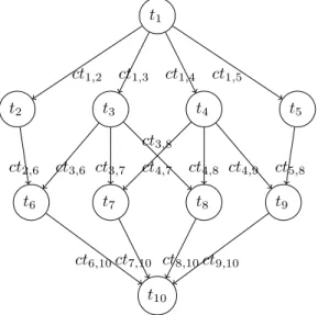
Acyclic Graph (DAG) orientedG(V, E), each vertex
repre-sents a taskti. Each arce ={ti, tj}represents a precedence
constraint between two tasksti andtj. We associate it with
the value cti,j which represents the communication delay
between ti and tj if they are executed on two different
resource types. The exact formula to evaluate cti,j which
takes into consideration latencies and available bandwidth between processors is provided in [28]. We denote by (i)
(resp. +(i)) the sets of the predecessors (resp. successors)
of taskti. Figure1presents an example of our application.
t1 t2 t3 t4 t5 t6 t7 t8 t9 t10 ct1,2 ct1,3 ct1,4 ct1,5 ct2,6 ct3,6 ct3,8 ct4,9 ct5,8 ct4,7 ct4,8 ct3,7 ct6,10ct7,10 ct8,10ct9,10
A task can be executed by a CPU or a GPU. Executing the task ti on a CPU (resp. GPU) generates an execution
time equal to wi,0 (resp.wi,1). A task ti can be executed
only after the complete execution of its predecessors. We do not allow duplication of tasks and preemption. We denote by
Cmaxthe completion time of the applicationA(makespan).
The aim is to find the minimum makespan of the application. Our problem can be modeled by mixed integer quadratic constrained program (P ). The decision variables are xi,j
and starti for i = 1..n and j = 1..m, wherexi,j = 1 if
ti is executed on the CPUj for j2 [1, `](resp. GPUj for
j2 [`+1, m]),0otherwise.startipresents the starting time
of the task ti.
The first constraint simply expresses that each task must be executed only once and on one processor. Constraints
(2) describes that the task ti2 must be executed after the
completion time of the taskti1for each taskti1that precedes
task ti2, and the communication cost cti1,i2 is added if
they are executed on two different processing elements. Constraint (3) is a disjunctive constraint to prohibit
over-lapping tasks on the same processor using a large constant
B, such that if two tasksti1andti2are executed on the same
processor, then eitherti2 starts after the completion time of
the task ti1 or ti1 starts after the completion time of the
taskti2. Constraints (4)describes thatCmaxis bigger than
the completion time of the tasks without successors. Thus, to minimize the finish execution time of the application, we must minimizeCmax.
(P ) 8 > > > > > > > > > > > > > > > > > > > > > < > > > > > > > > > > > > > > > > > > > > > : Pm j=1xi,j= 1,8i = 1..n (1) starti1+ xi1,j1wi1,b`+1j1c+ xi1,j1xi2,j2cti1,i26 starti2 (2) 8 i1 ! i2, 8j1= 1..m, 8j2= 1..m, j16= j2 starti1+ xi1,jwi1,b`+1j c6 starti2+ B⇥ (1 xi1j⇥ xi2j) _ (3) starti2+ xi2,jwi2,b`+1j c6 starti1+ B⇥ (1 xi1j⇥ xi2j) 8i1, i2= 1..n i16= i2, 8j = 1..m, B = Cte starti+ Pm j=1xi,jwi,b j `+1c6 Cmax,8i, +(i) =; (4) Z(min) = Cmax
4. Approximation algorithm for scheduling
DAG applications
In this section, we propose a two-phase approximation algorithm, aiming for a ratio of 6. We start by solving an assignment problem to find which processor (CPU or GPU) will execute each task. We propose two models(P 1)
and (P 2) for solving the assignment problem while the
precedence constraints are satisfied. The solution obtained by the model(P 1)or(P 2)represents a lower bound for the
final makespan. Then we solve the relaxation (P 10) (resp.
(P 20)) of the model (P 1) (resp. (P 2)). And in order to obtain a feasible assignment for the tasks, we rounded up the fractional solution of the program (P 10)and(P 20). In the second phase, we use the assignment of the tasks and list scheduling algorithm to get a feasible schedule.
4.1. Phase 1: assignment of tasks
4.1.1. Mathematical model.
Let the decision variablexi which is equal to 1 if the task
ti is assigned to a CP U and 0 otherwise. Let the two
binary variableszi,j andyi,j such thatzi,j = 1if the tasks
ti andtj are assigned to a CP U andyi,j = 1if the tasks
ti andtj are assigned to a GP U. LetCi be the finish time
of the taskti. The goal is to minimize the makespan.
(P 1) 8 > > > > > > > > > > > > > > > > > > > < > > > > > > > > > > > > > > > > > > > : Ci+ xjwj,0+ (1 xj)wj,1+ ⇣i,j6 Cj (1)
⇣i,j= (1 |yi,j zi,j|)cti,j,8(ti, tj)2 E
zi,j6 xi,8(ti, tj)2 E (2)
zi,j6 xj,8(ti, tj)2 E (3)
yi,j6 1 xi,8(ti, tj)2 E (4)
yi,j6 1 xj,8(ti, tj)2 E (5)
xiwi,0+ (1 xi)wi,16 Ci,8i = 1..n, (i) =; (6)
06 Ci6 Cmax,8i = 1..n, +(i) =; (7)
Pn
i=1xiwi,06 `Cmax (8)
Pn
i=1(1 xi)wi,16 kCmax (9)
xi, yi,j, zi,j2 {0, 1}, 8i = 1..n, j = 1..n (10)
Z(min) = Cmax
The model is inspired by the model given in [20]. Constraints (1 to 7) describes the critical path, such as if taskti precedestj, and these two tasks are assigned to two
different processors, we obtain two cases: eitherxi = 1and
xj = 0or xi= 0and xj = 1. In the two cases, we obtain
yi,j = 0 and zi,j = 0, implies that 1 |yi,j zi,j| = 1
because of the four constraints (2), (3), (4) and (5). If tasksti andtj are assigned to the same processor, we
obtain also two cases:
case 1: xi = 0 andxj = 0: in this case, zi,j = 0
and yi,j takes the value 1 (minimization problem),
then1 |yi,j zi,j| = 0.
case 2: xi = 1 and xj = 1 : in this case, yi,j = 0
and zi,j takes the value 1 (minimization problem),
then1 |yi,j zi,j| = 0.
Tasks without predecessors (respectively successors) are considered in the constraint (6) (resp. (7)). Constraint (8) (resp, (9)) simply expresses that the makespan cannot be smaller than the average load of work putted in CPUs (resp. GPUs). Note that the problem of finding the optimal mapping that minimizes makespan is np-hard even for the problem without communications delays [14], [25].
The first constraint contains an absolute value that can be processed in the CPLEX APIs [17]. In theC + +API,
Cplex.abs can be used. To see the efficiency of CPLEX
in managing the absolute value, we have proposed another model (P 2)without absolute value. By adding two binary
variablesai,j and bi,j and two constraints (5.1) and (5.2),
we can get rid of the absolute value, we obtain a second model(P 2).
The models (P 1)and (P 2)are equivalent. Indeed, the value of variablebi,j replace |yi,j zi,j| 2 {0.1}in(P 2),
1) |yi,j zi,j| = 0:2ai,j>bi,j and2(1 ai,j)>bi,j,
thenbi,j = 0for ai,j2 {0, 1}.
2) |yi,j zi,j| = 1: if(yi,j zi,j) = 1,1 + 2ai,j>bi,j
and 1 + 2(1 ai,j)>bi,j, and sincebi,j 2 {0.1},
bi,j = 1 for ai,j = 0. If (zi,j yi,j) = 1, 1 +
2ai,j >bi,j and 1 + 2(1 ai,j)>bi,j, and since
bi,j 2 {0.1},bi,j= 1 for ai,j= 1.
(P 2) 8 > > > > > > > > > > > > > > > > > > > > > > > < > > > > > > > > > > > > > > > > > > > > > > > : Ci+ xjwj,0+ (1 xj)wj,1+ ⇣i,j6 Cj (1)
⇣i,j= (1 bi,j)cti,j,8(ti, tj)2 E
zi,j6 xi,8(ti, tj)2 E (2)
zi,j6 xj,8(ti, tj)2 E (3)
yi,j6 1 xi,8(ti, tj)2 E (4)
yi,j6 1 xj,8(ti, tj)2 E (5)
(zi,j yi,j) + 2(1 ai,j)> bi,j,8(ti, tj)2 E (5.1)
(yi,j zi,j) + 2ai,j> bi,j,8(ti, tj)2 E (5.2)
xiwi,0+ (1 xi)wi,16 Ci,8i = 1..n, (i) =; (6)
06 Ci6 Cmax,8i = 1..n, +(i) =; (7)
Pn
i=1xiwi,06 `Cmax (8)
Pn
i=1(1 xi)wi,16 kCmax (9)
xi, yi,j, zi,j, ai,j, bi,j2 {0, 1}, 8i = 1..n, j = 1..n (10)
Z(min) = Cmax
In the following, we focus on the model(P 1), the results found for(P 1)remain valid for (P 2).
4.1.2. Relaxed problem. We obtain the model (P 10) by
relaxing the integrity variables xi, yi,j and zi,j. We also
obtain the model (P 20) by relaxing the integrity variables xi, yi,j, zi,j and bi,j. However, ai,j must remain integer.
We denote byy0i,j,z
0
i,j,b
0
i,j all in[0, 1], the fractional value
ofyi,j,zi,j,bi,j in the optimal solution of the model(P 1
0
)
or (P 20), with i = 1..n and j = 1..n. We denote by x0i
the fractional value of the assignment variable of task ti
in the optimal solution of the model (P 10) or (P 20). If x0i is integer for i2 1..n, the solution obtained is feasible
and optimal for (P 1) and (P 2), otherwise the fractional values are rounded. We denote byxr
i the rounded value of
the fractional value of the assignment variable of taskti in
the optimal solution of (P 10) or (P 20). We set xr i = 0 if
x0i<12,x r
i = 1 otherwise.
Let ✓1 be the mapping obtained by this rounding.
Each task ti is mapped in either CPU or GPU. Thus,
✓1(ti) ! {CP U, GP U}.
Proposition 1. The rounding previously defined satisfies the following two inequalities:
xr i 62x 0 i (1 xr i)62(1 x 0 i). Proof: If 06x0i < 12, thenxri = 062x 0 i. Further-more,2x0i61, then061 2x 0 i, follows xri = 061 2x 0 i, then 1 xr i 62(1 x 0 i). If 12 6x 0 i then1 62x 0 i, follows xr i = 1 6 2x 0 i. Furthermore, x 0 i 6 1 then 2x 0 i > 2, follows 1 2x0i > 1, then xr i = 1 6 1 2x 0 i, then 1 xr i 62(1 x 0 i).
Lemma 1. Let Cmax0 be the optimal solution obtained by
solving the programs(P 10)or(P 20). We can get another solution Cmax00 = C
0
max, such that for each two tasks ti
precedes tj: 1) if min{1 x0i, 1 x 0 j}> min{x 0 i, x 0 j}, then y 0 i,j= min{1 x0i, 1 x 0 j}andz 0 i,j = 0. 2) if min{1 x0i, 1 x 0 j} <min{x 0 i, x 0 j}, theny 0 i,j= 0
andzi,j0 =min{x
0
i, x
0
j}.
Proof: By constraints (2) and (3) from (P 10) or
(P 20) , z0i,j 6 min{x
0
i, x
0
j}. By constraints (4) and (5)
from (P 10) or (P 20), yi,j0 6 min{1 x
0 i, 1 x 0 j}. Let = |yi,j0 z 0
i,j|. To minimize the communication cost
(⇣i,j = (1 |y
0
i,j z
0
i,j|)cti,j) between ti and tj, we have
to maximize . = |yi,j0 z 0 i,j| 6 max{y 0 i,j, z 0 i,j} 6 max{min{1 x0i, 1 x 0 j},min{x 0 i, x 0 j}}. Then, if min{1 x0i, 1 x 0 j}> min{x 0 i, x 0
j}, then we can puty
0 i,j=min{1 x0i, 1 x 0 j} andz 0
i,j= 0 to maximize . Otherwise, we can
putzi,j0 =min{x
0 i, x 0 j}andy 0 i,j= 0.
In the following, we suppose that the solution obtained by solving the programs(P 10)or(P 20)follows the properties
given by the Lemma 1.
Let two tasks ti and tj, such that ti precedes tj. Let
↵i,jthe value given by↵i,j= 1 |y
0
i,j z
0
i,j|with replacing
y0i,j and zi,j0 by their values obtained by model (P 10) or
(P 20). In the following, we look for the relation between the value of↵i,j and the assignment of the tasksti andtj.
Remark 1.↵i,j>0. Indeed, ify
0 i,j=min{1 x 0 i, 1 x 0 j}6
1 and zi,j0 = 0, then ↵i,j = 1 y
0 i,j >0. Furthermore, if z0i,j = min{x 0 i, x 0 j} 6 1 and y 0
i,j = 0, then ↵i,j =
1 z0i,j>0.
Lemma 2. Ifti and tj are executed by two different
pro-cessing elements, then↵i,j >12.
Proof: Let two tasks ti and tj executed on two
different processing elements, we obtain two cases: a. x0i < 12 and x
0
j > 12: from constraints (2) and (3),
zi,j0 < 12. Furthermore,1 x
0
i>12 and1 x
0
j 612,
then, from constraints (4) and (5),y0i,j612. Finally,
↵i,j= 1 |y
0
i,j z
0
i,j|>1 max{yi,j, zi,j}> 12.
b. x0i > 12 and x
0
j < 12: from constraints (2) and (3),
zi,j0 < 12. Furthermore,1 x
0
i612 and1 x
0
j >12,
then, from constraints (4) and (5),y0i,j612. Finally,
↵i,j= 1 |y
0
i,j z
0
i,j|>1 max{yi,j, zi,j}> 12.
Let two tasks ti and tj, such that ti precedes tj. We
denote by Costr
i,j the value given by Costri,j = 0 if
xr
Proposition 2.Costr
i,j62↵i,jcti,j.
Proof: Iftjandtj are executed by the same
process-ing element,Costr
i,j= 062↵i,jcti,j, because↵i,j >0. If
tj andtj are executed by two different processing elements,
then Costr
i,j = cti,j. Then, from the lemma 2, ↵i,j > 12,
then2↵i,j>1, followsCosti,jr = cti,j62↵i,jcti,j.
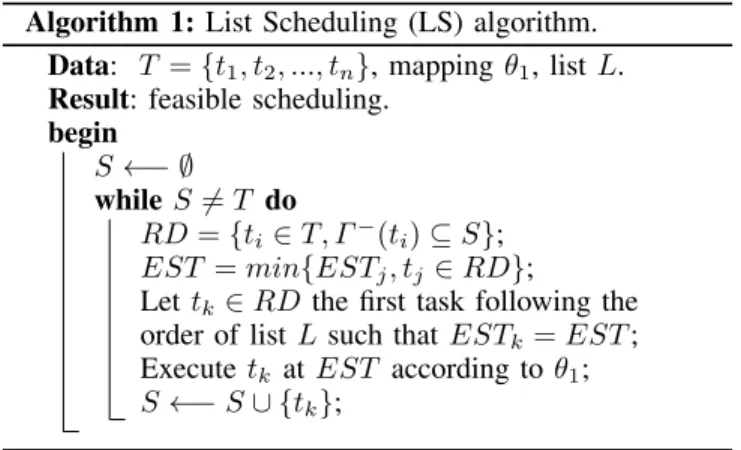
4.2. Phase 2: scheduling algorithm
We note by ESTi the Earliest Start Time of the task
ti according to the mapping ✓1. The following algorithm
builds a feasible schedule. The mapping✓1is used to define
on which processing element to execute which task (CPU or GPU). The algorithm determines for a task order given by a listL, the corresponding scheduling by executing the first
task ready of the list as long as there are free processing elements.
Algorithm 1: List Scheduling (LS) algorithm. Data: T ={t1, t2, ..., tn}, mapping✓1, list L.
Result: feasible scheduling. begin
S ;
whileS6= T do
RD ={ti2 T, (ti)✓ S};
EST = min{ESTj, tj2 RD};
Lettk 2 RDthe first task following the
order of listLsuch that ESTk= EST;
Executetk atEST according to✓1;
S S [ {tk};
The listL can be defined by different way, n!lists are
possible. In the following, we propose some lists that will be used for the experimentations.
4.2.1. List by using the model (P 10) or(P 20). Two
interesting lists extracted from the resolution of model
(P 10)or (P 20)can be used for algorithm 2, LST (List by
Start Time) andLF T (List by Finish Time). TheLST (resp. LF T) list can be obtained by sorting the tasks in
ascend-ing order of their processascend-ing start time (resp. processascend-ing finish time) obtained by solving the model(P 10)or (P 20).
Let Start0i (resp. C
0
i) be the processing start time (resp.
processing finish time) of the task ti obtained by
solv-ing the model (P 10)or (P 20), i = 1..n. Thus, LST = {t1, t2, ..., tn}, with Start 0 1 6 Start 0 2 6 ... 6 Start 0 n. LF T ={t1, t2, ..., tn}, withC 0 16C 0 26...6C 0 n.
4.2.2. List by longest path (LLP). In the first, we start
by defining graphG0(V, E), withV ={t
1, t2, ..., tn}andE
represent the set of graph edges. The vertices are labelled by the execution time of each task according to their assign-ments. The edges are labelled by the communication costs if ti precedes tj and xi 6= xj, 0 otherwise. Then, we can
calculate the longest pathP Li from each taskti to its last
successor. The listLLP is given byLLP ={t1, t2, ..., tn},
such thatP L1>P L2>...>P Ln.
4.3. Algorithm analysis
4.3.1. Lower bound. We note byCmax0 the optimal solution
obtained by(P 10)or (P 20), this solution is a lower bound
for the optimal solution of our problem C? max. C
0
max is
bounded by:
1) L(Pf): length of the fractional critical path
Pf in the optimal solution of the program
(P 10)or (P 20). 2) WCP Uf
` : The fractional weight of the tasks allocated
to the CPU in the optimal solution of the pro-gram (P 10)or (P 20)divided by`, withWCP Uf =
Pn i=1x
0
iwi,0.
3) WGP Uf
k : The fractional weight of the tasks allocated
to the GPU in the solution of the optimal program (P 10)or (P 20) divided by k, with WGP Uf =Pni=1(1 x0i)wi,1.
Furthermore, the solution bCmax obtained by Algorithm
1is bounded byL(Pr), W r CP U ` , Wr GP U
k , length of the critical
pathPrand the works on CPUs divided by`and the works
on GPUs divided bykin the final scheduling.
4.3.2. Worst case approximation ratio. We note by A
(resp. I) the cumulative sum of periods of activity (resp. inactivity) where the processors are busy (resp. idle) . Let
A1=Pni=1xriwi,0 (resp.A2 =Pni=1(1 xri)wi,1) be the
cumulative sum of periods of activity of all CPUs (resp, GPUs),A = A1+ A2. Let I1 (resp.I2) be the cumulative
sum of periods of inactivity where all CPUs (resp. GPUs) are busy and all GPUs (resp. CPUs) are idle. The maximum duration where all CPUs (resp. GPUs) are busy is A1
` (resp. A2 k ), thenI16k A1 ` (resp.I26` A2
k ). LetI3the cumulative
sum of periods of inactivity where at least one CPU and one GPU are idle,I = I1+ I2+ I3. Figure 2 represents the
occupation of processing elements. during the scheduling of an application.
Figure 2: Occupation of processing elements. By multiplying bCmax by the number of processors,
we find the cumulative sum of the periods of activity and inactivity,(` + k)Cbmax= A + I
We look now for the ratio between bCmax and Cmax? .
For this purpose, we try to limitAandI with formulas in functions ofC?
Proposition 3.
A162`Cmax?
A262kCmax? .
Proof: By definition, A1 = Pni=1xriwi,0. From
Proposition 1, xr i 6 2x
0
i. Then, A1 = Pni=1xriwi,0 6
Pn i=12x
0
iwi,0 = 2WCP Uf 6 2`C
0
max 6 2`Cmax? .
Fur-thermore, by definition, A2 = Pni=1(1 xri)wi,1. From
Proposition 1,(1 xr i)62(1 x 0 i). Then,A2=Pni=1(1 xr i)wi,1 6 Pni=12(1 x 0 i)wi,1 = 2WGP Uf 6 2kC 0 max 6 2kC? max.
Corollary 1. If for each task ti, xri is integer, such that
xri = x
0
i and(1 xri) = (1 x
0
i)for i = 1..n, then the
mapping✓1 is optimal. Follow, A1 = Pni=1xriwi,0 =
Pn i=1x
0
iwi,06`Cmax? andA2 =Pni=1(1 xri)wi,1=
Pn i=1(1 x 0 i)wi,16kCmax? . Corollary 2. I162kCmax? I262`Cmax? . Proof: I1 6 kA`1 6k2`C ? max ` = 2kC ? max. Furthermore, I2 6 `A2 k 6 2k`C? max k = 2`C ? max. Proposition 4.I362(` + k)Cmax? .
Proof: There exists a critical path in the final scheduling such that the sum of the instants where at least one CPU and one GPU are idle is less than2L(Pf). Indeed,
we assume that the tasks are stalled on the left. Let t0 be
the last task, such as during the execution oft0, there is an
idle CPU and an idle GPU. Let Start0 be the processing
start time of the task t0. If there is an idle CPU and idle
GPU beforeStart0, thent0 has a predecessort1 that ends
before Start0, the idle slots between Start1 and Start0
are covered either by the execution time of the task t1
and eventually the communication cost betweent1 and his
successor t00 which can bet0or a task on the path fromt1
tot0. If there is an idle CPU and idle GPU beforeStart1,
thent1 has a predecessort2that ends beforeStart1 which
can be obtained in the same precedent way. Let t0, t
0
0,
t1, t
0
1,..., t` be the maximum sequence of tasks obtained.
There is no more slots before Start` where at least one
CPU and one GPU are idle. Let the path containing all these tasks which covers all periods when at least one CPU and one GPU are idle, let L( ) its length. From Proposition 1, for any task ti in Pr, the processing time
of ti in the final scheduling will be at most twice the
fractional solution obtained by the program(P 10)or (P 20). For any two tasks ti, tj in Pr, from the Proposition 2,
the communication cost Costr
i,j between ti and tj in the
final scheduling will increase by at most twice the frac-tional communication cost↵i,jcti,jobtained by the program
(P 10)or (P 20). Then, L( )6L(Pr) = Pti2Pr(xriwi,0+ (1 xr i)wi,1) +P(ti,tj)2PrCost r i,j 6 P ti2Pr(2x 0 iwi,0+
2(1 x0i)wi,1) +P(ti,tj)2Pr2↵i,jcti,j 62L(Pf). Finally,
I36(` + k)L(Pr)62(` + k)L(Pf)62(` + k)Cmax? .
Theorem 1. The ratio between the solution bCmax obtained
by Algorithm1(LS) and the optimal scheduling solution C? max is given by b Cmax C? max 66.
Proof: bCmax = A+I`+k = A1+A2+I`+k1+I2+I3. Then,
from Proposition 3, 4 and Corollary 2, bCmax 6 (2`+2k+2k+2`+2(`+k))C? max `+k = 6Cmax? . Finally, b Cmax C? max 6 6.
Corollary 3. If the mapping✓1 is optimal, then CCbmax? max 65.
Proof:
From Corollary 1, we know that A1 6 `Cmax? and
A2 6 kCmax? . Then, bCmax = A1+A2+I`+k1+I2+I3 6 (`+k+2k+2`+2(`+k))C? max `+k . Finally, b Cmax C? max 65. 4.4. Iterative mapping
In order to find a more efficient rounding than ✓1
de-scribed previously, we try to assign the tasks progressively. Let✓2 be the rounding obtained by the following algorithm
2.
Algorithm 2: Rounding algorithm.
Data: model(P ) ((P 10)or(P 20)), >2. Result: mapping✓2. begin fori = 1tob2cdo SolveP; forj = 1 tondo if x0j < (i)then Set in P : x0j = 0 if x0j >1 (i)then Set in P : x0j = 1 forl = 1 ton do if x0l< 1 2 then xr l = 0 else xr l = 1
For a given integer v > 2, we solve the model (P 10)
or (P 20) b2c times adding new assignment constraint at each resolution. Contrary to✓1, we try to assign the tasks
progressively, starting by settingx0j to0 if x0j < (1) and
x0j to1if xj0 >1 (1)for the first resolution of (P 10
) or
(P 20), and finishing by setting x0j to0 if x0j < (b2c)and
x0j to 1 if x0j > 1 (b2c), where b2c 6 1
2 according to
Remark 2. For = 2, we obtain the rounding ✓1.
Lemma 3. For an integer v>2, bv2c
v 6 1 2. Proof: 1)v is even,v = 2 : bv2c v =2 = 1 2 2)v is odd,v = 2 + 1 : bv2c v = 2 +1 < 1 2. Remark 3.
The specialized accelerator problem can be solved with the same method, where a set of tasksT0 2 T can be executed by either a CPU or a GPU only. We denote bywi the execution time of each task ti2 T
0
. In fact, assuming that a task ti 2 T
0
is executable only by a CPU (resp. GPU), we can putwi,0= wiandwi,1= Cte
(resp.wi,0 = Cte and wi,1 = wi) where Cte is a big
value (we can putCte =Pti2T \T0max{wi,0, wi,1} +
P
ti2T0wi+
P
(tj,tk)2Ectj,k). With this transformation,
the rounding✓1 or✓2 will automatically assign the task
ti to the CPU (resp. GPU).
5. Numerical results
In this section, we compare the performance of LS (List Scheduling) algorithm to HEFT using benchmarks generated by Turbine [11]. In what follows, we describe the generation of benchmarks, then we discuss the efficiency of models
(P 10) and (P 20), the behavior of the algorithm 2 starting from mapping ✓1 and ✓2 using the different lists given in
section 4.
5.1. Benchmark
TABLE 1: Description of applications and platforms.
Instances Number of Platform 1 Platform 2
tasks ` k ` k test 1 10 3 3 1 1 test 2 30 4 4 1 1 test 3 60 4 4 1 1 test 4 100 6 6 1 1 test 5 200 6 6 1 1 test 6 400 6 6 1 1 test 7 500 8 8 1 1 test 8 600 8 8 1 1 test 9 800 8 8 1 1 test 10 1000 12 12 1 1
The benchmark is composed of ten parallel DAG appli-cations. We denote bytest iinstance numberi, we generate 10different applications for eachtest iwithi = 1..10. The
execution times of the tasks are generated randomly over an interval [wmin, wmax],wmin has been fixed at5andwmax
at30. The degree of the tasks are generated randomly over
an interval [dmin, dmax],dminhas been fixed at1anddmax
at10.
Furthermore, communication rate for each arc was gen-erated on an interval [ctmin, ctmax], we set ctmin to 35
andctmax to50. Table 1 presents the size of each instance
generated as well as the number of CPUs and GPUs used to execute each instance. For Platform1, we add more CPU and GPU by increasing the size of applications. For Platform2, we only use one CPU and one GPU.
5.2. Environment and algorithms
To study the performance of our method, we compared the ratio between each makespan value obtained by LS algo-rithm with HEFT algoalgo-rithm, the optimal solution obtained by CPLEX and the lower boundCmax0 obtained by(P 1
0
)
or(P 20).
Table 2 (resp. 3) shows the results of tests of LS al-gorithm on 10 instances for each application size given in
column Inst using three lists (LST, LF P, LLP) with the
rounding ✓1 (resp. ✓2) in platform 1. For the rounding ✓2,
we setv = 10. The next three columns concern the result of LS algorithm usingLST, where the column GAP gives
the average ratio between makespan obtained by LS algo-rithm andCmax0 ,GAP = LS makespan C
0 max
Cmax0 ⇥ 100. Column
Best presents the number of instances where LS algorithm provides better or the same solution obtained by using list
LST instead of LF T or LLP. Column Opt presents the
number of instances where LS provides optimal solution usingLST. We take the number of solutions equal to the optimal solution provided by CPLEX or to the value of the lower boundCmax0 obtained by (P 1
0
)or (P 20) if we have not optimal solution. Thus, we do the same thing for the listsLF T andLLP. Column Best LS with✓1 (resp. Best
LS with ✓2) presents the number of instances where LS
algorithm provides better or the same solution obtained by using the rounding ✓1 (resp. ✓2) and the best list of three
lists (LST,LF T,LLP) compared to the solution obtained by HEFT and LS algorithm using ✓2 (resp. ✓1) and all
lists (LST,LF T,LLP). Finally, column Time(P 10)(resp. Time(P 10)) gives the average time that was needed for LS
algorithm to provide a solution using the model(P 10)(resp. (P 20)) for the first phase.
Table 4 shows the results of tests of HEFT algorithm and running time of CPLEX in the same platform. Column Time CPLEX presents average time that was needed to CPLEX to provide the optimal solution using(P ). We only
have the result for the first two instances due to the large running time (> 14h). The next four columns concern the HEFT algorithm, where the column GAP gives the average ratio between makespan obtained by HEFT algorithm and
Cmax0 , GAP = HEFT makespan C
0 max
Cmax0 ⇥ 100. Column Opt
presents the number of instances where HEFT provides optimal solution. We take the number of solutions equal to the optimal solution provided by CPLEX or to the value of the lower boundCmax0 obtained by (P 1
0
Column Best HEFT presents the number of instances where HEFT algorithm provides better or the same solution obtained by using LS algorithm using the rounding✓1or✓2
for the three lists (LST,LF T,LLP). Finally, column Time
HEFT presents the average time that was needed for HEFT to provide a solution. A line Average is added at the end of each table which represents the average of the values each column. Table 5, 6 and 7 present the same results obtained for platform 2.
5.3. Results analysis
5.3.1. Platform 1. Obtaining the optimal solution using
CPLEX is very expensive in term of running time. For example, instance test 3 with 60 tasks and 4 GPU and 4 CPU, CPLEX cannot provide the optimal solution after 14h. Thus, we compare our method to the optimal solution
for only the first two instances. From Table 2 and 3, we can notice that list LLP is better than LF T and LST. Comparing to table 4 results, LS algorithm provides better solution than HEFT using rounding✓1or ✓2with listLF T
orLLP. Furthermore, LS algorithm using rounding✓2 and
list LLP is the most efficient method, with 78% of best solutions and a ratio of 7.33% comparing to the lower bound.
Inst LST LF T LLP Best LS Time
Gap Best Opt Gap Best Opt Gap Best Opt with✓1 P 1
0 P 20 test 1 0% 10 10 0% 10 10 0% 10 10 10 0.04s 0.06s test 2 4.51% 3 3 3.31% 4 4 2.35% 8 5 6 0.01s 0.11s test 3 17.61% 0 / 17.98% 0 / 11.25% 8 / 5 0.10s 0.16s test 4 13.39% 1 / 13.43% 1 / 7.38% 7 / 4 0.29s 0.35s test 5 27.69% 2 / 26.06% 2 / 15.93% 7 / 6 0.76s 0.67s test 6 25.93% 3 / 25.36% 3 / 12.82% 4 / 1 4.52s 2.64s test 7 28.23% 1 / 26.6% 2 / 14.32% 6 / 2 6.11s 3.75s test 8 22.79% 0 / 22.39% 1 / 11.51% 9 / 0 8.28s 4.85s test 9 14.87% 0 / 14.07% 0 / 2.204% 10 / 3 10.82s 5.47s test 10 20.55% 0 / 18.90% 1 / 5.32% 9 / 0 13.55s 6.65s Average 17.55% 20% / 16.81% 22% / 8.30% 78% / 37% 4.44s 2.47s TABLE 2: LS algorithm results using three lists (LST,LF P,LLP) with rounding ✓1 in platform1.
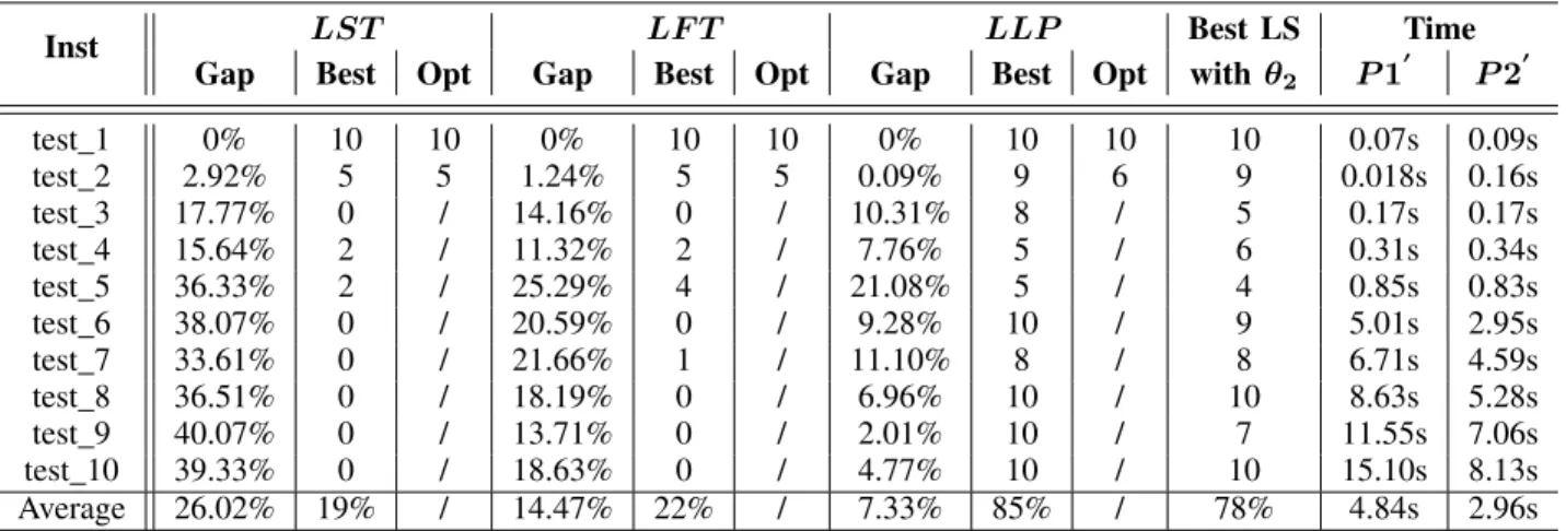
Inst LST LF T LLP Best LS Time
Gap Best Opt Gap Best Opt Gap Best Opt with✓2 P 1
0 P 20 test 1 0% 10 10 0% 10 10 0% 10 10 10 0.07s 0.09s test 2 2.92% 5 5 1.24% 5 5 0.09% 9 6 9 0.018s 0.16s test 3 17.77% 0 / 14.16% 0 / 10.31% 8 / 5 0.17s 0.17s test 4 15.64% 2 / 11.32% 2 / 7.76% 5 / 6 0.31s 0.34s test 5 36.33% 2 / 25.29% 4 / 21.08% 5 / 4 0.85s 0.83s test 6 38.07% 0 / 20.59% 0 / 9.28% 10 / 9 5.01s 2.95s test 7 33.61% 0 / 21.66% 1 / 11.10% 8 / 8 6.71s 4.59s test 8 36.51% 0 / 18.19% 0 / 6.96% 10 / 10 8.63s 5.28s test 9 40.07% 0 / 13.71% 0 / 2.01% 10 / 7 11.55s 7.06s test 10 39.33% 0 / 18.63% 0 / 4.77% 10 / 10 15.10s 8.13s Average 26.02% 19% / 14.47% 22% / 7.33% 85% / 78% 4.84s 2.96s TABLE 3: LS algorithm results using three lists (LST,LF P,LLP) with rounding✓2 in platform1.
TABLE 4: HEFT algorithm results and CPLEX running time for platform 1.
Instances CPLEXTime GapHEFTOpt HEFTBest HEFTTime
test 1 5m 11.08% 5 5 0.01s test 2 8h 13.48% 4 4 0.01s test 3 / 22.16% / 2 0.02s test 4 / 16.33% / 3 0.02s test 5 / 19.31% / 4 0.04s test 6 / 16.72% / 0 0.09s test 7 / 15.05% / 1 0.15s test 8 / 15.05% / 0 0.20s test 9 / 11.79% / 0 0.33s test 10 / 15.26% / 0 0.64s Average >4h 15.62% / 19% 0.15s
For the running time, HEFT algorithm needs less time than LS algorithm to provide a solution, where the first iteration of rounding algorithm (✓2) takes the same time
than✓1 (remark 2). Finally, we notice that the model(P 2
0
)
is more efficient than(P 10)in running time using rounding ✓1 or ✓2, where LS algorithm gives a solution in less than
3 seconds for instances of 1000 tasks using model (P 20),
while it need more than4seconds using model(P 10). Thus
5.3.2. Platform2. For this platform, we use only one CPU
and one GPU. CPLEX is more efficient than on the platform
1, but running time is still large. For instance test 3 with 60tasks, CPLEX cannot provide the optimal solution after 6h. Thus, we compare our method to the optimal solution
for only the first two instances. From Table 5 and 6, we can notice that list LLP is better than LF T and LST. Comparing to table 7 results, LS algorithm provides better solution than HEFT using rounding✓1or ✓2with listLF T
orLLP. Furthermore, LS algorithm using rounding✓2 and
list LLP is the most efficient method, with 76% of best solutions and a ratio of 9.86% comparing to the lower bound. For the running time, HEFT algorithm also needs less time than LS algorithm to provide a solution. Finally, unlike the platform 1, we notice that the model (P 10) is
more efficient than (P 20) in running time using rounding ✓1 or ✓2, where the LS algorithm gives a solution in less
than 1 second for instances of1000tasks for the two models.
Inst LST LF T LLP Best LS Time
Gap Best Opt Gap Best Opt Gap Best Opt with✓1 P 1
0 P 20 test 1 18.57% 7 5 18.57% 7 5 17.61% 8 5 8 0.04s 0.08s test 2 52.72% 1 1 49.55% 1 1 41.05% 6 3 5 0.30s 0.31s test 3 44.14% 0 / 41.18% 0 / 30.69% 6 / 5 0.35s 0.35s test 4 25.00% 0 / 24.02% 0 / 9.80% 7 / 6 0.05s 0.06s test 5 5.94% 2 / 5.93% 3 / 0.33% 10 / 10 0.07s 0.08s test 6 0.31% 8 / 0.31% 8 / 0.31% 10 / 4 0.40s 0.59s test 7 1.59% 8 / 1.54% 8 / 0.34% 10 / 4 0.27s 0.37s test 8 0.19% 10 / 0.19% 10 / 0.19% 10 / 8 0.38s 0.47s test 9 0.61% 9 / 0.39% 9 / 0.05% 10 / 5 0.64s 0.72s test 10 0.16% 9 / 0.16% 10 / 0.16% 10 / 5 0.88s 0.90s Average 14.92% 54% / 14.18% 56% / 10.05% 87% / 60% 0.33s 0.39s TABLE 5: LS algorithm results using three lists (LST,LF P,LLP) with rounding✓1 in platform2.
Inst LST LF T LLP Best LS Time
Gap Best Opt Gap Best Opt Gap Best Opt with✓2 P 1
0 P 20 test 1 17.26% 8 6 17.26% 8 6 16.30% 9 6 9 0.07s 0.09s test 2 55.68% 1 1 49.07% 1 1 43.03% 6 3 3 0.33s 0.35s test 3 60.16% 0 / 39.38% 0 / 29.21% 6 / 5 0.40s 0.40s test 4 41.96% 0 / 23.31% 0 / 9.11% 9 / 9 0.11s 0.14s test 5 20.52% 0 / 6.22% 2 / 0.43% 10 / 7 0.17s 0.23s test 6 11.41% 0 / 0.15% 8 / 0.15% 10 / 10 0.62s 0.82s test 7 8.73% 0 / 1.68% 8 / 0.19% 10 / 8 0.52s 0.82s test 8 8.08% 2 / 0.11% 10 / 0.11% 10 / 9 0.77s 1.13s test 9 10.90% 0 / 0.44% 9 / 0.03% 10 / 8 1.25s 1.89s test 10 8.67% 0 / 0.08% 10 / 0.08% 10 / 8 1.32s 1.91s Average 24.33% 11% / 9.96% 56% / 9.86% 90% / 76% 0.55s 0.77s TABLE 6: LS algorithm results using three lists (LST,LF P,LLP) with rounding✓2 in platform2.
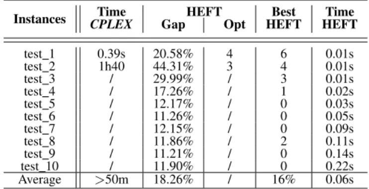
TABLE 7: HEFT algorithm results and CPLEX running time for platform2.
Instances CPLEXTime GapHEFTOpt HEFTBest HEFTTime
test 1 0.39s 20.58% 4 6 0.01s test 2 1h40 44.31% 3 4 0.01s test 3 / 29.99% / 3 0.01s test 4 / 17.26% / 1 0.02s test 5 / 12.17% / 0 0.03s test 6 / 11.26% / 0 0.05s test 7 / 12.15% / 0 0.09s test 8 / 11.86% / 2 0.11s test 9 / 11.21% / 0 0.14s test 10 / 11.90% / 0 0.22s Average >50m 18.26% / 16% 0.06s
6. Conclusion
This paper presents an efficient approximation algorithm to solve the task scheduling problem on hybrid platform with communication delays. We have studied the case of scheduling applications presented by DAG (Directed Acyclic Graph), the objective is to minimize the total execu-tion time (makespan). The main contribuexecu-tion of this work is a 6-approximation algorithm (LS) with two phases: mapping then assignment. Two models and two rounding strategies have been proposed for the mapping. In the second phase, a list scheduling algorithm has been proposed to generate a feasible schedule using several lists. LS algorithm guar-antees a ratio of 6 compared to the optimal solution using
the first strategy of rounding ✓1. Tests on large instances
close to reality demonstrated the efficiency of our method and shows the limits of solving the problem with a solver such as CPLEX.
As part of the future, we will try to study the tight of LS algorithm using rounding ✓2 which provide interesting
solutions. Then, we will focus on solving the problem with energy constraint due to the significant consumption of these platforms. An extension to more general heterogeneous platforms with more than two types of processor is also planned.
References
[1] https://www.top500.org/lists/2017/11/.
[2] Ishfaq Ahmad and Yu-Kwong Kwok. On exploiting task duplication in parallel program scheduling. IEEE Transactions on Parallel and Distributed Systems, 9(9):872–892, 1998.
[3] Massinissa Ait Aba, Lilia Zaourar, and Alix Munier. Approximation algorithm for scheduling a chain of tasks on heterogeneous systems. In Euro-Par 2017: Parallel Processing Workshops. Santiago de Com-postela, Spain, September 2017.
[4] Shaikhah AlEbrahim and Imtiaz Ahmad. Task scheduling for het-erogeneous computing systems. The Journal of Supercomputing, 73(6):2313–2338, 2017.
[5] Marcos Amaris, Giorgio Lucarelli, Cl´ement Mommessin, and Denis Trystram. Generic algorithms for scheduling applications on hybrid multi-core machines. In European Conference on Parallel Processing, pages 220–231. Springer, 2017.
[6] Hamid Arabnejad and Jorge G Barbosa. List scheduling algorithm for heterogeneous systems by an optimistic cost table. IEEE Transactions on Parallel and Distributed Systems, 25(3):682–694, 2014. [7] Rashmi Bajaj and Dharma P Agrawal. Improving scheduling of tasks
in a heterogeneous environment. IEEE Transactions on Parallel and Distributed Systems, 15(2):107–118, 2004.
[8] Olivier Beaumont, Lionel Eyraud-Dubois, and Yihong Gao. Influence of tasks duration variability on task-based runtime schedulers. 2018. [9] Olivier Beaumont, Lionel Eyraud-Dubois, and Suraj Kumar. Ap-proximation proofs of a fast and efficient list scheduling algorithm for task-based runtime systems on multicores and gpus. In Parallel and Distributed Processing Symposium (IPDPS), 2017 IEEE Inter-national, pages 768–777. IEEE, 2017.
[10] Luiz F Bittencourt, Rizos Sakellariou, and Edmundo RM Madeira. Dag scheduling using a lookahead variant of the heterogeneous earli-est finish time algorithm. In Parallel, Distributed and Network-Based Processing (PDP), 2010 18th Euromicro International Conference on, pages 27–34. IEEE, 2010.
[11] Bruno Bodin, Youen Lesparre, Jean-Marc Delosme, and Alix Munier-Kordon. Fast and efficient dataflow graph generation. In Proceedings of the 17th International Workshop on Software and Compilers for Embedded Systems, pages 40–49. ACM, 2014.
[12] Cristina Boeres, Vinod EF Rebello, et al. A cluster-based strategy for scheduling task on heterogeneous processors. In Computer Architec-ture and High Performance Computing, 2004. SBAC-PAD 2004. 16th Symposium on, pages 214–221. IEEE, 2004.
[13] Louis-Claude Canon, Loris Marchal, and Fr´ed´eric Vivien. Low-cost approximation algorithms for scheduling independent tasks on hybrid platforms. In European Conference on Parallel Processing, pages 232–244. Springer, 2017.
[14] Philippe Chretienne. Task scheduling with interprocessor communi-cation delays. European Journal of Operational Research, 57(3):348– 354, 1992.
[15] Fabi´an A Chudak and David B Shmoys. Approximation algorithms for precedence-constrained scheduling problems on parallel machines that run at different speeds. Journal of Algorithms, 30(2):323–343, 1999.
[16] Michael R Garey and Ronald L. Graham. Bounds for multiprocessor scheduling with resource constraints. SIAM Journal on Computing, 4(2):187–200, 1975.
[17] IBM. Ibm ilog cplex v12.5 user’s manual for cplex,
http://www.ibm.com. 2013.
[18] E Ilavarasan, P Thambidurai, and R Mahilmannan. High performance task scheduling algorithm for heterogeneous computing system. In ICA3PP, volume 2005, pages 193–203. Springer, 2005.
[19] Muhammad Kafil and Ishfaq Ahmad. Optimal task assignment in heterogeneous distributed computing systems. IEEE concurrency, 6(3):42–50, 1998.
[20] Safia Kedad-Sidhoum, Florence Monna, and Denis Trystram. Scheduling tasks with precedence constraints on hybrid multi-core machines. In Parallel and Distributed Processing Symposium Work-shop (IPDPSW), 2015 IEEE International, pages 27–33. IEEE, 2015. [21] Minhaj Ahmad Khan. Scheduling for heterogeneous systems using constrained critical paths. Parallel Computing, 38(4-5):175–193, 2012.
[22] Minhaj Ahmad Khan. Task scheduling for heterogeneous systems using an incremental approach. The Journal of Supercomputing, 73(5):1905–1928, 2017.
[23] Sunita Kushwaha and Sanjay Kumar. An investigation of list heuristic scheduling algorithms for multiprocessor system. IUP Journal of Computer Sciences, 11(2):29, 2017.
[24] Samantha Ranaweera and Dharma P Agrawal. A task duplication based scheduling algorithm for heterogeneous systems. In Parallel and Distributed Processing Symposium, 2000. IPDPS 2000. Proceed-ings. 14th International, pages 445–450. IEEE, 2000.
[25] Linshan Shen and Tae-Young Choe. Posterior task scheduling algo-rithms for heterogeneous computing systems. In International Con-ference on High Performance Computing for Computational Science, pages 172–183. Springer, 2006.
[26] Haluk Topcuoglu, Salim Hariri, and Min-you Wu. Performance-effective and low-complexity task scheduling for heterogeneous com-puting. IEEE transactions on parallel and distributed systems, 13(3):260–274, 2002.
[27] Shuli Wang, Kenli Li, Jing Mei, Guoqing Xiao, and Keqin Li. A reliability-aware task scheduling algorithm based on replication on heterogeneous computing systems. Journal of Grid Computing, 15(1):23–39, 2017.
[28] Lilia Zaourar, Massinissa Ait Aba, David Briand, and Jean-Marc Philippe. Modeling of applications and hardware to explore task mapping and scheduling strategies on a heterogeneous micro-server system. In Parallel and Distributed Processing Symposium Workshops (IPDPSW), 2017 IEEE International, pages 65–76. IEEE, 2017.