HAL Id: hal-01101501
https://hal.archives-ouvertes.fr/hal-01101501
Submitted on 9 Jan 2015
HAL is a multi-disciplinary open access archive for the deposit and dissemination of sci-entific research documents, whether they are pub-lished or not. The documents may come from teaching and research institutions in France or abroad, or from public or private research centers.
L’archive ouverte pluridisciplinaire HAL, est destinée au dépôt et à la diffusion de documents scientifiques de niveau recherche, publiés ou non, émanant des établissements d’enseignement et de recherche français ou étrangers, des laboratoires publics ou privés.
Macroscopic modelling of urban floods
Vincent Guinot, Carole Delenne
To cite this version:
Vincent Guinot, Carole Delenne. Macroscopic modelling of urban floods. La Houille Blanche - Revue internationale de l’eau, EDP Sciences, 2014, 6, pp.19-25. �10.1051/lhb/2014058�. �hal-01101501�
MACROSCOPIC MODELLING OF URBAN FLOODS
Vincent GUINOT(1), Carole DELENNE(1)(1)Université Montpellier 2 / HSM UMR 5569, [email protected],[email protected]
Modelling urban floods at the scale of the conurbation remains a challenging task owing to the size ratio between the hydraulic features and the modelling domain. Upscaling makes such modelling possible. Macroscopic models allow CPU and model pre-processing times to be divided by 102 to 103 compared to classical models. Macroscopic inundation fields may be interpolated for finer scale simulations. Four types of macroscopic urban flood models are currently available from the literature: the single porosity model, the integral porosity approach, the conveyance reduction factor model and the multiple porosity model. Analysing the four formulations indicates that they can be expected to exhibit significantly different behaviour in a variety of hydraulic configurations. So far, they have been applied to different types of urban layouts or only compared to numerical simulations. Identifying the best formulations call for a systematic experimental benchmarking involving steady state and transient regimes.
Key words: Urban flood, inundation, two-dimensional model, upscaling,
porosity models
MODELISATION MACROSCOPIQUE DES INONDATIONS
URBAINES
Le ratio entre les échelles du détail hydraulique pertinent et de la zone urbaine rend la simulation des crues urbaines difficilement envisageable à l’échelle de l’agglomération. Le transfert d’échelle rend possible ce type d’opération. Les modèles macroscopiques permettent typiquement un gain de temps de calcul d’un facteur 102 à 103 par rapport aux modèles détaillés. Ils sont obtenus à partir des modèles à surface libre classiques par des opérations de prise de moyenne. Ils permettent de produire des champs inondants à des échelles de l’ordre de la centaine de mètres. Ces champs peuvent être réutilisés comme conditions aux limites de modèles détaillés, de taille plus réduite. Les quatre modèles macroscopiques proposés jusqu’à présent dans la littérature sont le modèle à porosité simple, le modèle à formulation intégrale, le modèle à réduction de débitance et le modèle à porosité multiple. L’analyse de leur formulation indique que leurs comportements devraient être assez différents dans un certain nombre de configurations. Cependant, ils ont été en général appliqués sur des situations différentes ou comparés uniquement à des simulations numériques. L’évaluation de leurs performances respectives appelle la réalisation de benchmarks expérimentaux systématiques, faisant intervenir sur les mêmes configurations géométriques des régimes permanents et des régimes transitoires.
Mots-clefs : Crues urbaines, inondation, modèle bidimensionnel, changement
d’échelle, modèles à porosité
I INTRODUCTION
Urban floods are characterised by highly variable flow fields and hydraulic configurations. Although one-dimensional modelling attempts have been reported in the literature [Mark et al., 1994], two-dimensional (2D) modelling of urban inundations is the most widely used approach [Bates et al., 2010; Bates and De Roo, 2000; Mignot et al., 2006]. While 2D models are seen as suitable tools for refined flow modelling over relatively small areas, the refined modelling of entire conurbations remains a technical issue. With a typical size of 10-1 to 1 m for the relevant hydraulic singularity, meshing an entire urban area of size 103 to 104 m would lead to 108 to 1010 computational cells. Besides the huge CPU requirement, pre-processing the computational grid is known to be a heavily man-supervised operation. Human supervision of meshing operations is a well-known costly budget line in a hydraulic study.
Macroscopic modelling appears as an interesting alternative. Using large-scale, statistical descriptors of the hydraulic properties of the urban medium allows a typical size of 10 m for the
cells, thus reducing the number of cells in a model by a factor 103 to 105. The macroscopically computed hydrodynamic fields may be interpolated and used as initial and boundary conditions for local, refined 2D modelling studies where a detailed knowledge of the flow features is required. A number of macroscopic models have been presented in the literature. They are based on averaging techniques. Averaging is not the only upscaling technique available from the literature. Powerful approaches, such as homogeneization via multiple scale expansions, have been applied successfully to hydrodynamics and transport in heterogeneous porous media [Bensoussan et al., 1978; Auriault and Adler, 1995]. They are however subjected to a number of constraints, among which the existence of a Representative Elementary Volume (REV) [Bear, 1998] and the scale separation principle [Auriault, 1991]. Such conditions are likely not to be fulfilled in practical applications [Guinot, 2012]. Besides, homogeneization is known to be meaningless for purely hyperbolic problems at the microscopic scale [Auriault and Adler, 1995], which is precisely the case of the shallow water equations.
Averaging techniques are also usually based on the existence of a REV. Practical applications [Guinot, 2012] as well as local formulations [Sanders et al., 2008] show however that the REV assumption may be relaxed.
The available macroscopic urban flood models are reviewed in Sections 2 to 5. Section 6 is devoted to a discussion of the validation requirements for these models and the need for systematic research effort.
II THE SINGLE POROSITY MODEL
II.1 Conceptual model
The single porosity model was first introduced by Defina et al. [1994]. Applications can be found in [Bates, 2000; Hervouët et al., 2000]. The governing equations were developed in a slightly different way in conservation form and implemented within a finite volume framework in Guinot and Soares-Frazão [2006]. Experimental validation of this model has been presented in [Lhomme, 2006; Lhomme et al., 2007; Soares-Frazão et al., 2008]. Further numerical developments have followed in the form of various numerical solvers for the porosity equations [Cea and Vazquez-Cendon, 2010; Finaud-Guyot et al., 2010].
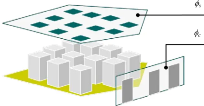
The single porosity shallow water model is obtained from an averaging over a two-dimensional control volume. Porosity is defined as the fraction of the area available to the flow and storage of water (Figure 1).
Figure 1. Porosity as the fraction of space available to water flow and storage.
From a conceptual point of view, two different porosities might be considered [Lhomme, 2006]: (i) a storage porosity φs that represents the plan view storage area, (ii) a connectivity porosity φc that accounts for the front area available to the flow. Elementary statistical considerations indicate that, assuming that the Reference Elementary Volume (REV) exists, the two porosities should be identical [Sanders et al., 2008], φs = φc = φ.
φs
II.2 Governing equations, head loss models
The governing equations are written in vector conservation form as
s f f u+∂ +∂ = ∂tφ xφ x yφ y (1a)
[
]
[
]
[
]
T y T x T gh hv huv hv huv gh hu hu hv hu h, , , = , 2+ 2/2, , = , , 2+ 2/2 = f f u (1b)(
)
(
)
[
]
T y y f y x x f x S gh gh S S gh S gh φ φ φ φ − + ∂ − + ∂ = 0, /2 , 0, , 2/2 2 , , 0 s (1c)where g is the gravitational acceleration, h is the water depth, u and v are respectively the x- and
y-flow velocities, S0,X and Sf,X are respectively the bottom and friction slopes in the X-direction
(X = x, y) and φ is the porosity.
It is easy to check that the wave propagation speeds in the single porosity shallow water model are the same as in the classical 2D shallow water equations. This can be viewed as a weakness of the single porosity model in that the presence of buildings has been reported to modify the wave propagation speeds significantly in urban areas [Liang et al., 2007].
In the first conservative version of the single porosity model [Guinot and Soares-Frazão, 2006], a specific head loss model had been proposed. The effect of urban singularities (junctions, vehicles, street bends, etc.) were accounted for by a Borda-like head loss model. This model was proposed on the basis of the Toce scale model experiment [Zech and Soares-Frazão, 2007], where the head losses at crossroads were attributed to the sudden street widenings at junctions. A close inspection of the refined, 2D modelled flow fields has indicated since then that this assumption was most probably erroneous [Guinot, 2012]. Lhomme [2006] proposed an alternative formulation based on a second-order tensor. The lack of experimental data did not allow this formulation to be validated. The most recent evolution of the head loss model is probably the fourth-order tensor formulation proposed by Velickovic [2012], that allows strongly anisotropic head loss patterns to be modelled.
III THE INTEGRAL POROSITY APPROACH
III.1 Conceptual model
Sanders et al. [2008] proposed an alternative formulation to the single porosity model. Like the single porosity model, the integral model is also derived by averaging the 2D shallow water equations over a control volume. In contrast with the single porosity approach, in the integral formulation the porosity is meaningful at the scale of the computational cell. A differential formulation for this model is meaningless. This has two advantages: (i) the integral approach does not require the existence of the REV, (ii) it allows the storage porosity to be distinguished from the connectivity porosity, the former and the latter being derived from a domain and contour integral respectively, as in Figure 1. Stagnant water-induced storage effects can thus be accounted for by this model, a feature that is absent from the single porosity model. The price to pay for the increased model flexibility is strongly mesh-dependent porosities, with the consequence that (i) the modeller should be sufficiently experienced in mesh design not to adopt the wrong mesh pattern, (ii) this precludes numerical convergence studies from being carried out. It is thus very difficult to determine whether a numerically computed solution is close to the exact one.
III.2 Governing equations, head loss model
As the term “integral” indicates, the governing equations are meaningful only when written for a control volume. Although meaningless in theory, the differential form is used hereafter for the sake of comparison with the single porosity model. The vector conservation form of the equations is
' s f f u+∂ +∂ = ∂tφs xφc x yφc y (2)
The difference with the single porosity model is the presence of two different porosity factors, φs for the conserved variable and φc for the fluxes. The Jacobian matrices of the fluxes fX (X = x, y) with respect to u are those of the classical 2D shallow water equations multiplied by φc/φs. This leaves the structure of the eigenvalues of the hyperbolic system unchanged, thus yielding the wave propagation speeds of the classical 2D shallow water model multiplied by the ratio φc/φs.
Sanders et al. [2008] proposed a drag coefficient-based head loss model. The drag coefficient is a function of building shape, orientation and spacing and usually requires calibration.
IV THE BUILDING COVERAGE RATIO/CONVEYANCE REDUCTION FACTOR (BCR/CRF) MODEL
IV.1 Conceptual model
The BCR/CRF model [Chen et al., 2012a-b] is an upscaled version of the 2D diffusive wave approximation. The governing assumptions are the following: (i) inertia is negligible in the momentum balance, (ii) the presence of buildings induces a reduction in the area available for storage via the BCR and (iii) a reduction in the conveyance via the CRF. The BCR and CRF are not necessarily identical and depend on building geometry, orientation and size, as in the integral model. The BCR and CRF exert a similar influence (with a difference in sign) on the flow properties as the porosities φs and φc respectively, as shown in the next section.
IV.2 Governing equations
The governing equations are the following
(
)
[
h]
x[
(
x)
qx]
y[
(
y)
qy]
S t − +∂ − +∂ − = ∂ 1 α 1 β 1 β (3a)(
S S)
S h X x y n q zx zy zX M X , , 1 5/3 , 2 / 1 2 , 2 , + = = − (3b)(
h z)
X x y z Sz,x ≡−∂X =−∂X + b , = , (3c) where α is the BCR, βx (X = x, y) is the CRF in the X-direction and S is a source term per unit area.The BCR and CRF influence both the propagation speed and spreading rate of the waves. For the sake of simplicity, the analysis is carried out for homogeneous BCR and CRF in one-dimensional configuration without mass source term. The system (3a-c) simplifies to
(
1−α)
∂th+(
1−βx)
∂xqx =0 (4a)(
S h)
n h q q x x M x x = 2 0, −∂ 3 / 10 (4b) Differentiating equations (4a) and (4b) with respect to space and time respectively gives(
1−α)
∂xth+(
1−βx)
∂xxqx =0 (5a) ∂ − ∂ = − ∂ = ∂ t x x t x x M x x M x t tx q h q h h q q n q q h n S h 2 13/3 13/3 3 / 10 2 , 0 2 3 10 (5b) Substituting equation (5b) into (5a), noticing that ∂ can be expressed as a function of th ∂xqx via equation (4a) yields0 1 1 1 2 1 1 3 10 2 3 / 13 3 / 13 − ∂ = − − ∂ + ∂ − − x xx x M x t x x x x x x q n q h q q h q q α β α β (6)
Simplifying leads to the following writing 0 = ∂ − ∂ + ∂tqx V xqx D xxqx
which is the classical diffusive wave formulation, where the propagation speed V and the diffusion coefficient D of the hydrograph are given by
x x u V α β − − = 1 1 3 5 (7a) x M x q n h D 2 3 / 10 1 1 2 1 α β − − = (7b)
where ux is the x-velocity.
Both V and D are proportional to (1 – βx)/(1 – α). Since the spreading of the hydrograph is proportional to (Dt)1/2, the CRF does not modify the propagation and spreading speeds of the hydrograph in the same way.
It is worth emphasizing the physical relevance of this model. Consider the idealized situation where long and narrow buildings are oriented perpendicular to the flow. This leads to a smaller ratio (1 – βx)/(1 – α) and subsequently to slower wave propagation and spreading than the same buildings oriented parallel to the flow. This is justified from a physical point of view by the larger lateral storage in the former situation compared to the latter.
It must be kept in mind, however, that diffusive wave models are well-suited for applications where the inertial terms are negligible. This model is thus adapted to the simulation of slow transients involving small velocities.
V THE MULTIPLE POROSITY MODEL
V.1 Conceptual model
The multiple porosity model [Guinot, 2012] was developed as a generalization of the single porosity model. The development of this model was strongly influenced by the remark by Sanders
et al. [2008] that the REV does not necessarily exist in an urban area, a statement that has been
confirmed since then [Guinot, 2012]. Any averaging procedure is thus bound to induce strong biases in the formulation. To overcome this problem, the choice was made to partition the flow domain into several regions with similar flow properties. In the most general proposed version of the multiple porosity model, the following regions are presented (Figure 2).
Figure 2. Definition sketch for the multiple porosity model (from [Guinot, 2012]). Ωb : buildings ; Ωm : isotropic mobile
region ; Ωs : stagnant region ; Ω1, Ω2 : anisotropic regions 1 and 2 (e.g. street networks) ; Ω1,2 :junctions between the
anisotropic regions 1 and 2.
– An immobile, impervious region Ωb where the water cannot penetrate.
Ωb Ωs Ωm Ω1 Ω2 Ω1,2
– An isotropic mobile region Ωm, where the wave propagation properties can be assumed isotropic. This is the case where the building orientation is random, with no identifiable preferential direction.
– A stagnant region Ωs accounting for dead zones (inner building yards, parking lots, dead ends, etc.)
– M anisotropic regions Ωk, k = 1,...,M where the flow is constrained along a preferential direction. Such regions represent the street network.
– Exchange regions Ωk,k’ between the anisotropic regions Ωk, Ωk’. These regions account for the junctions between the street networks. In practical applications of the model, such regions have been found superfluous [Guinot, 2012].
Each of these regions has its own hydrodynamic state variables. Two different regions are liable to exchange mass and momentum. So far, an extremely simple exchange model [Guinot, 2012] based on free surface elevation differences has been seen to work satisfactorily.
V.2 Governing equations
Averaging the shallow water equations over each of the regions yields the following set of equations m g m f m y m y x m x m tU +∂ F +∂ F =S +S +Q ∂ ( ) ( ) , , (8a) s s tU =Q ∂ (8b) M k k g k f k k x k t k , 1, , ) ( ) ( = + + = ∂ + ∂ U F S S Q (8c)
[
]
T m m m m m m m =φ h ,h u ,h v U , Us =[ ]
φshs , Uk =φk[
h ,k hkuk]
T (8d)[
]
T m m m m m m m m m x m h u ,h u gh /2,h u v 2 2 , =φ + F , my m[
hmvm,hmumvm,hmvm ghm/2]
T 2 2 , =φ + F (8e)[
]
T k k k k k k u ,u h gh /2 2 2 + =φ F , m[
f x f y]
T f m S , S , ) ( , , 0 φ = S ,[
f k]
T f k S , ) ( , 0 = S (8f)[
]
T m y m y m m m x m x m m g m 0,( h S h /2)g,( h S h /2)g 2 , 0 2 , 0 ) ( = φ + ∂ φ φ + ∂ φ S , Qm =φm[
Em,Gm,x,Gm,y]
T (8g)[
s s]
s = φ E Q ,[
]
k k[
k k]
T T k x k k k k g k 0,( h S h k )g , E ,G 2 , 0 ) ( = φ + ∂ φ =φ Q S (8h)where ED and GD (D = m, s, k = 1,…,M) are respectively mass and momentum source terms arising from the exchange between the various regions and the coordinate xk is taken along the preferential direction of the region k. Transferring a mass ED per unit time from the region D to the other regions yields a momentum transfer GD = EDuD.
In the isotropic mobile region m, the wave propagation speeds are the same as in the classical 2D shallow water equations. In the anisotropic regions, only one-dimensional wave propagation is possible and the wave propagation speeds are those of the 1D Saint Venant equations. The wave speed is zero in the stagnant region, that is non-connected by definition. The coupling between the various regions induces a modification in the wave speeds owing to the source terms ED and GD. A simplified version of the model can be derived under the Local Equilibrium Assumption (LEA) that equilibrium between the water levels in all the regions is achieved instantaneously at all points [Guinot, 2012]. Interestingly enough, the wave propagation speeds are different depending on whether the domain is emptying or filling.
V.3 Head loss model
The momentum source term classically accounts for bottom friction via a Manning/Strickler law. In [Guinot, 2012] the building drag-induced head loss model is that proposed by Sanders et
It must be noted, however, that the multiple porosity model intrinsically embeds an additional energy dissipation mechanism. When water is transferred from a region to another, the corresponding momentum is transferred too. Transferring mass from a mobile region (be it isotropic or anisotropic) to the stagnant region causes instantaneous momentum cancellation. The kinetic energy attached to the transferred water vanishes immediately. Transferring mass from a mobile region to any of the anisotropic regions also cancels the component of the momentum in the direction orthogonal to the main direction of the receiving region, thus dissipating part of the kinetic energy instantaneously. When water is transferred from the stagnant region to one of the mobile regions, the overall momentum is preserved but the velocity decreases owing to the increase in the mobile mass. All these mechanisms contribute significantly to the head loss terms. As a matter of fact, all the numerical experiments carried out so far have shown that the exchange mechanism suffices to account for all head losses, without the need for the drag term proposed in [Sanders et al. 2008].
V.4 Application example: single, integral and multiple porosity models
The present application illustrates the difference between the behaviours of the single and multiple porosity models. Both models are applied to the Toce test case reported in [Soares-Frazão and Zech, 2007]. As mentioned in Section IV.2, applying the diffusive wave-based BCR/CRF approach to this test case would be meaningless because inertial terms play a predominant role in the flow equations. In this test case, the breaking of a dam is simulated experimentally by injecting water into the scale model from the upstream end (left-hand side of the model in Figure 3). Figure 3a shows the contour lines of the topography. The main channel clearly is visible in the Northern part of the floodplain. In the scale model experiment, an idealized urban area was implemented in the form of 5×4 square building blocks aligned along the main floodplain direction.
Figure 3b shows the contour lines of the free surface elevation computed using a classical 2D shallow water model at t = 20 s after the beginning of the injection. Several features may be noted: (i) a bore propagating in the upstream direction from the Western side of the urban area, with an asymmetrical shape, the Nothern part of the bore propagating farther than the Southern part; (ii) an increase in the free surface gradient on both sides of the urban area; (iii) an asymmetrical, triangular wake downstream of the idealized city
Figure 3c shows the water levels computed at t = 20 s using the single porosity model presented in Section 2. The three abovementioned features can be identified, but (i) the extension of the upstream travelling bore is strongly underestimated, (ii) the free surface gradient spreads over a much larger distance than in the refined 2D model, (iii) the shape of the downstream wake is not triangular as in the refined 2D model.
Figure 3d shows the water levels computed at t = 20 s using the integral porosity model presented in Section 3. Compared to the single porosity model, the integral approach exhibits significant improvements. More specifically, the extent of the upstream bore is much better approximated (compare Figs 3b and 3d). This, however, is achieved at the expense of overestimated depths at the upper left corner of the urban area and strongly underestimated depths in the river bed. The free surface gradient computed by the integral porosity model remains significantly stronger in the city than that computed by the refined 2D model.
Figure 3e shows the free surface contour lines obtained using the multiple porosity model. Two anisotropic regions are used in this model, one for each street direction. The building-induced head loss coefficient proposed by [Sanders et al., 2008] is set to zero, the head losses being accounted for only by the Manning-Strickler bottom friction model and the mass/momentum exchange processes between the two anistropic regions. As mentioned in Section V.3, the exchange between the anistropic regions suffices to account for all the head losses in the multiple porosity model. Comparing it with Figure 3b shows that (i) the extension and orientation of the upstream travelling bore is correctly reproduced, (ii) the free surface gradient on both sides of the idealized city is
reproduced correctly, with the denser contour lines located on the downstream part of the left-hand side of the city, (iii) the triangular shape of the downstream wake is restored.
In terms of model processing and CPU performance, the refined 2D model presented in Figure 3b counts more than 4.8×10⁴ cells, against 4.6×10³ for the porosity models. The porosity models run 75 times faster than the refined 2D model.
Figure 3. Toce test case. (a) scale model topography (contour line spacing 0.5 mm). (b) free surface elevations computed by a 2D shallow water model at t = 20 s (contour line spacing 1 cm). (c) free surface elevations computed by the single porosity model (contour line spacing 1 cm). (d) free surface elevations computed by the integral porosity model (contour line spacing 1 cm). (e) free surface elevation computed by the multiple porosity model (contour line spacing 1 cm). Plan view coordinates in metres.
(a) 1 2 3 4 5 6 4 5 6 7 8 7.5 7.55 7.6 7.65 zb (m) (b) (c) 1 2 3 4 5 6 4 6 8 7.54 7.56 7.58 7.6 7.62 7.64 z (m) 1 2 3 4 5 6 4 6 8 7.54 7.56 7.58 7.6 7.62 7.64 z (m) (d) (e) 1 2 3 4 5 6 4 6 8 z (m) 7.54 7.56 7.58 7.6 7.62 7.64 1 2 3 4 5 6 4 6 8 z (m) 7.54 7.56 7.58 7.6 7.62 7.64
VI DISCUSSION – CONCLUSIONS
Substantial research effort has been devoted to the derivation of macroscopic urban flood models over the past decade. Macroscopic, porosity-based shallow water models operate from 102 to 103 times faster than their classical counterparts, thus appearing as a promising alternative for the study of urban floods at the scale of the entire urban area. The theoretical analysis presented in this paper shows that the four existing types of macroscopic model should be expected to behave differently in transient mode. Determining which approach performs better for which range of flow configuration requires extensive validation. So far, however, these four models have only be validated against rather limited data sets over a very narrow range of configurations. Bringing this type of model to the operational stage requires that research be pursued under two lines.
1. Systematic laboratory validation involving the widest possible range of hydraulic and geometric conditions. For instance, the single, integral and multiple porosity model have been applied to a single common test case, the Toce experiment. This comparison involves only one flow experiment, with a single layout for aligned buildings. The BCR/CRF model has not been compared to the shallow water-based, porosity models. Besides, the head loss mechanisms embedded in the multiple porosity model suggest that some models may give a similar response under quasi-steady conditions, while exhibiting very different behaviours under transient conditions. Both quasi-steady and transient flow configurations should thus be tested systematically over the same geometric configurations.
2. Developing pre-processing tools that would allow the macroscopic descriptors of the urban area (porosity, main street network directions) to be derived from standard products, such as urban databases or high-resolution DEMs [Chen et al., 2012a-b; Gallien et al. 2011].
VII REFERENCES
Auriault J.L. (1991). – Heterogeneous medium. Is an equivalent macroscopic description possible ? Int. J. Eng. Sci., 29: 785-795.
Auriault J.L., Adler P. (1995). – Taylor dispersion in porous media: analysis by multiple scale expansions. Adv. Wat. Res. 18: 217-226.
Bates P.D. (2000). – Development and testing of a sub-grid scale model for moving boundary hydrodynamic problems in shallow water. Hydrological Processes, 14: 2073-2088.
Bates P.D., Horritt M.S., Fewtrell T.J. (2010). – A simple inertial formulation of the shallow water equations for efficient two-dimensional flood inundation modelling. J. Hydrol., 387: 33-45.
Bates P.D., De Roo A.P.J. (2000). – A simple raster-based model for flood inundation simulation.
J. Hydrol., 236: 54-77.
Bear J. (1998). – Dynamics of fluids in porous media. Dover Publications Inc., NY.
Bensoussan A., Lions J.L., Papanicolaou G. (1978). – Asymtotic analysis for periodic structures. North-Holland, Amsterdam, The Netherlands.
Cea L., Vazquez-Cendon M.E. (2010). – Unstructured finite volume discretization of two-dimensional depth-averaged shallow water equations with porosity, Int. J. Numer. Meth. Fluids, 63: 903-930.
Chen A., Evans B., Djordjevic S., Savic D.A. (2012a). – A coarse-grid approach to represent building blockage effects in 2D urban flood modelling, J. Hydrol., 426-427: 1-16.
Chen A., Evans B., Djordjevic S., Savic D.A. (2012b). – Multi-layer coarse-grid modelling in 2D urban flood simulations, J. Hydrol., 470: 1–11.
Defina A., D'Alpaos L., Mattichio B. (1994). – A new set of equations for very shallow water and partially dry areas suitable to 2D numerical models, Proceedings Specialty Conference “Modelling
Flood Propagation over Initially Dry Areas”, Ed. P. Molinaro and L. Natale, , Am. Soc. Civ. Eng.,
Finaud-Guyot P., Delenne C., Lhomme J., Guinot V., Llovel C. (2010). – An approximate-state Riemann solver for the two-dimensional shallow water equations with porosity. Int. J. Numer.
Meth. Fluids, 62: 1299-1331.
Gallien T.W., Schubert J.E., Sanders B.F. (2012). – Predicting tidal flooding of urbanized embayments: A modeling framework and data requirements. Coastal Engineering, 58: 567-577.
Guinot V. (2012). – Multiple porosity shallow water models for macroscopic modelling of urban floods, Adv. Wat. Resour., 37: 40-72.
Guinot V., Soares-Frazão S. (2006). – Flux and source term discretization in two-dimensional shallow water models with porosity on unstructured grids. Int. J Numer. Meth. Fluids, 50: 309-345.
Hervouët J.-M., Samie R., Moreau B. (2000). – Modelling urban areas in dam-break flood-wave numerical simulations, Proc. International Seminar and Workshop on Rescue Actions Based on
Dambreak Flow Analysis, Seinâjoki, Finland, 1–6 October 2000.
Lhomme J. (2006). – Modélisation des inondations en milieu urbain. Approches unidimensionnelle, bidimensionnelle et macroscopique. PhD thesis, Université Montpellier 2.
Lhomme J., Soares-Frazão S., Guinot V., Zech Y. (2007). – Modélisation à grande échelle des inondations urbaines et modèle 2D à porosité. La Houille Blanche, 04-2007: 104-110.
Liang D., Falconer R.A., Lin B. (2007). – Coupling surface and subsurface flows in a depth averaged flood wave model, J. Hydrol. 337: 147-158.
Mark O., Weesakul S., Apirumanekul C., Aroonet S.B., Djordjevic S. (2004). – Potential and limitations of 1D modelling of urban flooding, J. Hydrol. 299: 284-299.
Mignot E., Paquier A., Haider S. (2006). – Modeling floods in a dense urban area using 2D shallow water equations, J. Hydrol., 327: 186-199.
Sanders B.F., Schubert J.E., Gallegos H.A. (2008). – Integral formulation of shallow water equations with anisotropic porosity for urban flood modelling. J. Hydrol., 362: 19-38.
Soares-Frazao S., Lhomme J., Guinot V., Zech Y. (2008). – Two–dimensional shallow water models with porosity for urban flood modelling. J. Hydr. Research, 46(1): 45-64.
Velickovic M. (2012). – Macroscopic modeling of urban flood by a porosity approach. PhD thesis, Université catholique de Louvain.
Zech Y., Soares-Frazao S. (2007). Dam-break flow experiments and real-case data. A database from the European IMPACT project, J. Hydr. Research, 45 (1): 5-7.
![Figure 2. Definition sketch for the multiple porosity model (from [Guinot, 2012]). Ω b : buildings ; Ω m : isotropic mobile region ; Ω s : stagnant region ; Ω 1 , Ω 2 : anisotropic regions 1 and 2 (e.g](https://thumb-eu.123doks.com/thumbv2/123doknet/13739538.437051/6.892.108.397.849.1046/figure-definition-multiple-porosity-buildings-isotropic-stagnant-anisotropic.webp)
