HAL Id: hal-03000632
https://hal.archives-ouvertes.fr/hal-03000632
Submitted on 17 Jan 2021
HAL is a multi-disciplinary open access
archive for the deposit and dissemination of
sci-entific research documents, whether they are
pub-lished or not. The documents may come from
teaching and research institutions in France or
abroad, or from public or private research centers.
L’archive ouverte pluridisciplinaire HAL, est
destinée au dépôt et à la diffusion de documents
scientifiques de niveau recherche, publiés ou non,
émanant des établissements d’enseignement et de
recherche français ou étrangers, des laboratoires
publics ou privés.
Distributed under a Creative Commons Attribution - NonCommercial| 4.0 International
License
Q. Jamet, A. Ajayi, J. Le Sommer, Thierry Penduff, A. Hogg, W. Dewar
To cite this version:
Q. Jamet, A. Ajayi, J. Le Sommer, Thierry Penduff, A. Hogg, et al.. On Energy Cascades in
Gen-eral Flows: A Lagrangian Application. Journal of Advances in Modeling Earth Systems, American
Geophysical Union, 2020, 12 (12), pp.e2020MS002090. �10.1029/2020MS002090�. �hal-03000632�
A Lagrangian Application
Q. Jamet1 , A. Ajayi1, J. Le Sommer1, T. Penduff1 , A. Hogg2 , and W. K. Dewar1,3
1Univ. Grenoble Alpes, CNRS, IRD, Grenoble INP, IGE, Grenoble, France,2Research School of Earth Sciences and ARC Centre of Excellence for Climate Extremes, Australian National University, Canberra, ACT, Australia,3Department of EOAS, Florida State University, Tallahassee, FL, USA
Abstract
An important characteristic of geophysically turbulent flows is the transfer of energy between scales. Balanced flows pass energy from smaller to larger scales as part of the well-known upscale cascade, while submesoscale and smaller scale flows can transfer energy eventually to smaller, dissipative scales. Much effort has been put into quantifying these transfers, but a complicating factor in realistic settings is that the underlying flows are often strongly spatially heterogeneous and anisotropic. Furthermore, the flows may be embedded in irregularly shaped domains that can be multiply connected. As a result, straightforward approaches like computing Fourier spatial spectra of nonlinear terms suffer from a number of conceptual issues. In this paper, we develop a method to compute cross-scale energy transfers in general settings, allowing for arbitrary flow structure, anisotropy, and inhomogeneity. We employ Green's function approach to the kinetic energy equation to relate kinetic energy at a point to its Lagrangian history. A spatial filtering of the resulting equation naturally decomposes kinetic energy into length-scale-dependent contributions and describes how the transfer of energy between those scales takes place. The method is applied to a doubly periodic simulation of vortex merger, resulting in the demonstration of the expected upscale energy cascade. Somewhat novel results are that the energy transfers are dominated by pressure work, rather than kinetic energy exchange, and dissipation is a noticeable influence on the larger scale energy budgets. We also describe, but do not employ here, a technique for developing filters to use in complex domains.1. Introduction
A surprising aspect of nonlinear geophysical flows, namely, that they transfer energy from smaller to larger scales and thus in a sense opposite to that of three-dimensional, isotropic turbulence, has been known for some time (Charney, 1971; Fjortoft, 1953; Kraichnan, 1967). The reason for this behavior has been traced to the quasi-two dimensionality of so-called balanced dynamics, which strongly constrains vortex tube stretch-ing. Scott and Wang (2005) argue for the observation of an upscale cascade in the ocean from analysis of satellite sea surface height measurements, and Scott and Arbic (2007) argue for the same in numerical models. Others have argued that this behavior in wavenumber space is accompanied by a transfer in the frequency domain to lower frequencies (Arbic et al., 2012) and extensions to the combined wavenumber frequency domain have also been found (Arbic et al., 2014).
An upscale cascade dynamically and importantly affects the ocean. For example, the transfer from high frequency mesoscale variability to low frequencies implicates eddies as a mechanism effecting climate variability (Berloff & McWilliams, 1999; Dijkstra & Molemaker, 1999; Holland, 1978). Further, the large-scale circulation receives energy from the large-scale, slowly evolving winds (Ferrari & Wunsch, 2009; Wunsch & Ferrari, 2004), and it is generally thought that this energy is shunted to the mesoscale by geostrophic instabilities. An equilibrated ocean must then find a pathway for the mesoscale to lose its energy, and the so-called upscale cascade presents a hindrance. The return of energy to larger scales where dissipation is vanishingly weak has led to considerable recent interest in mesoscale energy loss.
Given that cross-scale energy exchange in the ocean is central to ocean and climate dynamics, it is important to examine how those transfers can be measured. Most energy exchange diagnoses of both observations and models have proceeded through the use of Fourier transforms (Arbic et al., 2014), which requires that the data be converted into forms consistent with the approach. Speaking primarily about spatial analyses,
Key Points:
• A method for computing cross-scale energy transfers for general settings is developed
• Potential to kinetic energy cross-scale exchanges are dominant • Dissipation is surprisingly strong as
an effect on large scales
Correspondence to: W. K. Dewar, [email protected]
Citation:
Jamet, Q., Ajayi, A., Le sommer, J., Penduff, T., Hogg, A., & Dewar, W. K. (2020). On energy cascades in general flows: A Lagrangian application. Journal of Advances
in Modeling Earth Systems, 12, e2020MS002090. https://doi.org/10. 1029/2020MS002090
Received 27 FEB 2020 Accepted 12 SEP 2020
Accepted article online 18 SEP 2020
©2020. The Authors.
This is an open access article under the terms of the Creative Commons Attribution License, which permits use, distribution and reproduction in any medium, provided the original work is properly cited.
geographically confined regions of interest are usually defined. Since the data are not spatially periodic, as assumed by Fourier methods, tapering or windowing is usually applied. The subsequent analysis then occurs on the windowed domain, and the results are in some sense representative of an averaged state-ment of the transfers in the domain. Another complicating factor is that irregularities can appear inside the domain. An example is Bermuda, sitting in the open Atlantic at a location near to the Gulf Stream and the separated North Atlantic jet. Methods, often subjective, are required to handle such areas, frequently involving an interpolation over the problematic regions. Nonetheless, these analyses have usually yielded answers consistent with our theoretical expectations. They do represent spatial averages however, and fur-ther understanding of inhomogeneous regions, like the Kuroshio and the Gulf Stream, requires more spatial resolution. This served in part as motivation for Aluie et al. (2018), who examined energy exchanges locally based on a purely spatial filtering approach.
The focus of this paper is to propose a new method for analyzing kinetic energy in models and observations that appears to avoid many of the above-mentioned issues with Fourier methods. It also differs from previous approaches in several ways, primarily in focussing on a Lagrangian-like approach and working directly with the kinetic energy equation. We apply the technique to primitive equation model output describing vortex merger and hence an upscale cascade. The results indicate an upscale cascade, thus demonstrating the via-bility of the procedure, even though it is not limited to this restrictive setting. The theoretical basis for the procedure is outlined in the next section; the model description and applications appear in the following section. We discuss and summarize the paper in the concluding section, emphasizing new results specific to the energetics of the upscale cascade and outline thoughts for further work. Methods to handle domain irregularities are outlined in Appendix A. An Eulerian version of the present analysis appears in Appendix B. Derivation of comparable formulas for potential energy are discussed in Appendix C, and modifications to the analysis introduced when using isopycnal coordinates are outlined in Appendix D.
2. An Analysis of the Kinetic Energy Equation
2.1. Overview
Below, we present an analysis of the kinetic energy equation. In brief, our plan is to apply Green's function analysis to the kinetic energy equation. The result relates the final kinetic energy of a parcel to its initial kinetic energy and its history along its (quasi-) Lagrangian trajectory. We then filter this equation in physi-cal space to obtain a statement about a length-sphysi-cale-based decomposition of the final kinetic energy. Similar filterings of the initial kinetic energy and kinetic energy sources then yield statements about cross-scale energy transfers. Finally, we average the pointwise kinetic energy decomposition to obtain a more represen-tative view of the cross-scale transfers. These steps are spelled out in sequence in the following subsections. The reader wishing to skip mathematical detail can go directly to Equations 36–38, where the results are summarized.
We begin with the hydrostatic equations in Cartesian coordinates, the zonal momentum component of which is
ut+uux+vu𝑦+wuz−𝑓v = −px+𝜈(uxx+u𝑦𝑦+uzz) (1) where u is zonal velocity and subscripts x, y, z, and t denote partial derivatives with respect to zonal, merid-ional, and vertical location and time, respectively. The quantity p is pressure, and𝜈 is viscosity. A partial step to constructing the kinetic energy equation involves multiplying Equation 1 by u, which results in
(u2∕2)
t+u(u2∕2)x+v(u2∕2)𝑦+w(u2∕2)z−𝑓uv
= −upx+ (𝜈(uux))x+ (𝜈(uu𝑦))𝑦+ (𝜈(uuz))z−𝜈(ux)2−𝜈(u𝑦)2−𝜈(uz)2
(2)
A similar procedure on the meridional momentum equation and adding returns the kinetic energy equation
Kt+ ∇⋅ uK = −uh⋅ ∇hp −𝜖 + ∇ ⋅ (𝜈∇K) (3) where K = u2∕2 + v2∕2 =|u
h|2∕2 and𝜖 = 𝜈∇uh⋅ ∇uh=𝜈|∇uh|2is dissipation. We rewrite this as
where R = −uh⋅∇hp −𝜖 contains the “sources” and “sinks” for kinetic energy. Given that pressure gradients
appear in the momentum equations as a force acting on a fluid particle, the quantity −uh⋅ ∇hprepresents
movement in the direction of a force. We will thus refer to it as “pressure work.” The quantity −𝜖 is simply dissipation of kinetic energy.
Exploiting the hydrostatic balance, pressure work can be rewritten as
−uh⋅ ∇hp = −∇⋅ up + wb (5) where b is buoyancy. The last quantity in Equation 5 is the exchange between kinetic and potential energy. In this paper, we work primarily with pressure work, noting that potential energy exchange is a component of pressure work.
2.2. Comparison to Other Approaches
Working directly with kinetic energy, via Equation 4, distinguishes this approach from others. Traditional Fourier analysis proceeds by transforming Equation 1 and multiplying by the momentum transform conju-gate û(k)∗where k denotes a wavenumber. The result (Ê(k) = (ûû∗+̂v̂v∗)∕2) is usually interpreted as the
energy spectrum, although more properly it is related to the momentum spectrum. The relation of Ê(k) to energy comes indirectly from Parseval's equality, i.e.,
∫V
Kdx = ∫
k
E(k)dk (6)
which, while useful, argues this approach is restricted to integral statements. In contrast, the Fourier transform of K is
̂K(k) = 1
2∫p
[û(p)û(k − p) +̂v(p)̂v(k − p)]dp (7) which, although quite different from Ê(k), still satisfies Parseval's identity while being directly related to kinetic energy.
To probe into the spatial structure of energy transfers, it is natural to remain in the physical domain. In this sense, our approach is like that of Aluie et al. (2018). We differ from them in that they “coarse-grain” Equation 1 and multiply by the coarse-grained velocity to obtain an equation describing ̄K =0.5(̄u2+̄v2),
where the bar denotes the coarsening operator. In the process, terms appear in the ̄Kequation involving third order quantities likēu(uux) −̄u(̄u ̄ux), which in the LES community are interpreted as measuring the
energy cascade due to wave-mean flow interaction. They describe the effect on ̄K, following a parcel moving at̄u, of subgrid-scale processes.
Clearly, the coarsening operator is one of the primary distinctions between Aluie et al. (2018) and the present approach. In fact, if we choose the coarsening operator as a Dirac delta function, then ̄u = u and our approaches merge. The cost of this choice is the wave-mean flow interaction term vanishes, leading to the statement that the unfiltered equations do not cascade. In our view, cascading is broader than wave-mean flow interaction and occurs in unfiltered results, as evidenced in Figure 1. The panels show results from the numerical model discussed in detail later in the paper. For now, we mention they are plots of kinetic energy in a layer and come from Days 20 and 585 of a doubly periodic numerical experiment typified by vortex merger. Both plots are in physical space and neither plot has been coarse-grained nor filtered. Visual comparison suggests that the later plot is characterized by larger length scales than the earlier. Spectra of “normalized” kinetic energy, i.e., of the variable𝜅 = a(t)K, for both days, taken along the line in Figure 1 (right), appear in Figure 2. The integrated kinetic energies along this line were used to normalize the kinetic energies, i.e., a(t) =(∫𝑦K(t)d𝑦)
−1
, so that the total integral in both plots,∫𝑦𝜅d𝑦, was unity. This was done to remove amplitude variations that would interfere with the comparisons of the wavenumber content. The earlier spectrum (red) is characterized by enhanced energies at higher wavenumbers, while the later (blue) shows elevated levels at lower wavenumbers. Clearly a “cascade” has occurred in these unfiltered plots, and it is this behavior we seek to quantify.
Although our procedure differs from that of Aluie et al. (2018), we do not criticize their approach. They adopt a procedure of clear relevance to modelers interested in parameterization. Our approach is meant for the full diagnosis of “eddy-resolving” models.
Figure 1. Distribution of kinetic energy in layer two of our four-layer model on (left) Year 0 Day 20 and Year 1 Day
220 (right).
2.3. Kinetic Energy at a Single Point
We now apply Green's function analysis, which leads eventually to the construction of kinetic energy at a point and begins by multiplying Equation 4 by some space-time-dependent function G.
GKt+G∇⋅ uK − G∇ ⋅ (𝜈∇K) = GR (8)
Straightforward calculus leads to
(GK)t+ ∇⋅ uGK − ∇ ⋅ (𝜈G∇K) + ∇ ⋅ (K𝜈∇G) −K(Gt+ ∇⋅ uG + ∇ ⋅ (𝜈∇G)) = RG
(9)
Again, appealing to straightforward Green's function methods, we suppose G satisfies
Gt+ ∇⋅ uG = −∇ ⋅ (̂𝜈∇G) − 𝛿(x − xo, t − to) (10) where𝛿 is the usual Dirac delta function centered on the so-called source points xo, toand̂𝜈 is a viscosity-like quantity. It is not necessarily equal to𝜈, although in this paper, we will always discuss cases where ̂𝜈 = 𝜈. Boundary conditions are required to solve Equation 10. As is typical for Green's functions, the boundary
Figure 2. Spectra of kinetic energy ̂Kfrom Year 0 Day 20 (red) and Year 1 Day 220 (blue). Clearly, a cascade of kinetic energy to larger scales has occurred in this unfiltered view of kinetic energy.
conditions will always be homogeneous; however, how they will be distributed between specified values of
Gand its normal derivatives on the boundary is yet to be determined.
Equation 10 is almost a simple advection-diffusion equation, differing only because viscosity appears multi-plied by −1, i.e., −̂𝜈 < 0, as opposed to ̂𝜈 > 0 occurs on the right-hand side. In fact, such a result is standardin Green's function analyses, where the equation solved by G is the adjoint of the equation governing K, and is handled by solving Equation 10 backwards in time. Instead of an initial condition, a “posterior” condition on G is applied, and integration proceeds to temporally earlier values. For this case, we will always choose a posterior condition of G(t𝑓) =0. Notationally, G = G(x, t; xo, to), expressing the dependence of G on both
the “source” points, xo, to, and the “observation” points, x, t.
Now, we perform an integral of Equation 9 over a volume V of the observation space, x, and over the time interval 0 to to, where 0< to. K(xo, to) − ∫ x GK(x, 0)dx + ∫ to 0 ∫S (uGK −̂𝜈G∇K + ̂𝜈K∇G) ⋅ ⃗ndSdt = ∫ to 0 ∫x RGdxdt + ∫ to 0 ∫x G∇⋅ ((𝜈 − ̂𝜈)∇K)dxdt (11)
where S is the surface bounding the volume V . At this point, we exploit the available flexibility in boundary conditions. Equation 11 describes how various kinetic energy sources contribute to the final kinetic energy at a point. From a physical perspective, we expect that kinetic energy transport across the boundary S can con-tribute to the final kinetic energy inside S. This can occur by kinetic energy advection and viscous exchange across S. Both of these appear in Equation 11 multiplied by G. We therefore choose to apply ∇G⋅ ⃗n = 0, i.e., homogenous Neumann boundary conditions, to G, thus eliminating the underlined term from Equation 11 and preserving the aforementioned physical effects.
Suppose first V is a closed domain. With this, and a rearrangement of terms, we obtain
K(xo, to) = ∫ x G(x, 0; xo, to)K(x, 0)dx + ∫ to o ∫x ̂RGdxdt (12) where ̂R = R + ∇ ⋅ ((𝜈 − ̂𝜈)∇K)
as the boundary fluxes all vanish.
Equation 12 illustrates how the kinetic energy at location xoand time tohas been constructed. The first term
on the right-hand side represents the “initial” kinetic energy, K(x, 0) that ends up at (xo, to). The volume defining the impact of this K(x, 0) contribution depends on the development of G from to. The last term involves the internal fluid sources of kinetic energy and how they have contributed to K along the trajectory that eventually ends up at xo. Equation 12 provides a full deconstruction of the kinetic energy in the basin, regardless of spatial inhomogeneities in the flow.
If V is an open domain or a subdomain of a full, closed basin, Equation 12 is augmented by advective and dif-fusive fluxes of kinetic energy across the subdomain boundary, to the extent they are involved as measured by G. These vanish identically in the presence of doubly periodic conditions, which will describe our appli-cation in this manuscript. But even for the most general case, boundary contributions can be made small by choosing a domain large enough that advection and diffusion do not have time to reach the boundaries. We will proceed here ignoring boundary contributions.
The clearest interpretation of this formula occurs if G, defined in Equation 10, measures purely Lagrangian trajectories, which occurs in the limit̂𝜈 = 0. For the remainder of this paper, we will continue with ̂𝜈 = 𝜈 both for simplicity and because our numerical application will employ a very small value for𝜈. We have also checked that our results are insensitive tô𝜈 < 𝜈. It is in the nearly Lagrangian nature of Equation 12 that the present approach somewhat resembles that of Nagai et al. (2015) and Shakespeare and Hogg (2017). K. Srinivasan has also alerted us to early contributions by Kraichnan (Kraichnan, 1964, 1967) in which Green's function-based analysis of turbulence was employed. There are similarities in our approaches, but the objec-tives our studies differ. Kelley et al. (2013) also explored the coarse-graining decomposition in Aluie et al. (2018) in a Lagrangian setting with a focus on Lagrangian Coherent Structures.
2.4. Cross-Scale Contributions to Kinetic Energy
We now compute how energy is transferred between various length scales. These exchanges become more complicated when K(xo, to) is strongly inhomogeneous and anisotropic, as is typical in the ocean. In this and
the next subsections, we will build to a formal statement of cross-scale transfers in several steps, proceeding from a statement valid at a single point to one averaged over a specified volume.
As a first step, consider a “filter” applied to K(xo, to), i.e.,
KL(x1, to) = ∫
xo
K(xo, to)𝑓L(xo−x1)dxo (13)
where fLis a filter associated with a length scale, L, and fixed at location x1. What the filter might be is
a question deserving discussion, because the filtering will be carried out in physical space. For realistic problems, physical space typically contains a lot of irregularity: examples are complex lateral boundaries and major topography that can extend through domains at given depths and reach up to the surface. Any useful filter must contend with these features. Guidance about the filters can be obtained from the simplest case of an unbounded domain without interior obstacles. In that case, as we argue below, the obvious choices are trigonometric functions. At a more fundamental level, these work because they are a collection of functions forming a complete set due to their being the eigenfunction, eigenvalue solutions to the Helmholtz equation in an unbounded domain. We argue in Appendix A basis functions constructed from the Helmholtz equation with homogeneous conditions on S, the boundary of the domain V , will for complex domains provide a collection of functions with the desired properties. We stress here, however, that Appendix A is not exploited in the present paper but serves as a procedure in need of further examination.
But whatever the filter is, an important point is that the filter works on the “source points” (xo) of Green's function. Operating on Equation 12, we obtain
KL(x1, to) = ∫ x GLK(x, 0)dx + ∫ to o ∫x RGLdxdt (14) where GL(x, t; x1, to) = ∫ xo G(x, t; xo, to)𝑓L(xo−x1)dxo (15) We can similarly filter Equation 10 to show
𝜕
𝜕tGL+ ∇⋅ uGL= −∇(𝜈 ⋅ ∇GL) −𝑓L(x − x1)𝛿(t − to) (16)
We want the filtering to decompose K(x1, to) completely into scale-dependent information, i.e.,
∫
∞
L=0
KL(x1, to)dL = K(x1, to) (17)
Employing Equation 13 in Equation 17, it is simple to show ∫
∞
L=0𝑓L
(xo−x1)dL =𝛿(xo−x1) (18)
where𝛿 is the Dirac delta function (This property of the basis set is essential to their role in filtering. We will revisit it in Appendix A when developing more general basis sets.). A classic result from the theory of generalized functions is ∫ ∞ −∞ e−2𝜋k⋅(xo−x1)dk = Π3 i=1∫ ∞ −∞ e−2𝜋ki(xi,o−xi,1)dk i=𝛿(xo−x1) (19)
where the index i denotes dimensions and Π implies multiplication. Working now with one of the dimen-sions, suppressing the subscript i, breaking the integral into real and imaginary parts, and using symmetry implies
2 ∫
∞
o
Last, we employ the relation between wavenumber and wavelength, k = 1∕L, to obtain 2 ∫ ∞ o cos(2𝜋(xo−x1)∕L) L2 dL =𝛿(xo−x1) (21)
which effectively defines our original filter, fL, for a single spatial dimension
𝑓L(xo−x1) =2 cos (2𝜋(x o−x1) L ) L2 (22)
To filter over a group of length scales Lx, Ly, and Lz in three dimensions, one employs the product of Equation 22 appropriate to each dimension. The quantity KL(x1, to) represents the energy resident in
K(x1, to) between the length scales L and L +𝛿L.
2.5. Band Pass Filtering of Final Kinetic Energy
The second step in formulating cross-scale transfers is to represent the energy at x1resident between scales of
Ljand Lkby suitable integration over length scales. For example, the energy at scales Ljand greater becomes
(again working in one dimension)
𝜅∞ L𝑗(x1, to) = ∫ ∞ L𝑗 KL(x1, to)dL = 2 L𝑗∫ ∞ −∞ sinc ( 2𝜋(xo−x1) L𝑗 ) K(xo, to)dxo (23) where sinc(x) = sin(x) x (24)
is the well-known “sinc” function, often found in signal detection applications. The remainder of the energy at shorter lengths is
𝜅L𝑗
o =K(x1, to) −𝜅L∞𝑗(x1, to) (25)
Analogous to Equation 15, we define ΓLk L𝑗(x, t; x1, to) = ∫ xo∫ Lk L𝑗 𝑓L (xo−x1)dL G(x, t; xo, to)dxo (26)
and find that it is governed by
𝜕 𝜕tΓ Lk L𝑗+ ∇⋅ uΓ Lk L𝑗 = −∇⋅ (𝜈∇Γ Lk L𝑗) −𝛾 Lk L𝑗(x1−x)𝛿(t − to) (27) where 𝛾Lk L𝑗(x1−x) = ∫ Lk L𝑗 𝑓L(x1−xo)dL (28)
This more general formulation anticipates that the length-scale-dependent basis functions needed to probe the scale-dependent structure of K in general domains will not typically be trigonometric functions. See Appendix A for more discussion. We will frequently refer to𝛾Lk
L𝑗 in the following as a “filter.”
The construction of the kinetic energy at x1between Ljand Lkcan be written
𝜅Lk L𝑗(x1, to) = ∫ x ΓLk L𝑗K(x, 0)dx + ∫ to o ∫x R(x, t)ΓLk L𝑗dxdt where 𝜅Lk L𝑗(x1, to) = ∫ Lk L𝑗 KL(x1, to)dL = ∫ Lk L𝑗 ∫x K(x, to)𝑓L(x − x1)dxdL (29)
Note that Equation 29 is a Lagrangian statement of kinetic energy exchange, in that the modified Green's function ΓLk
to use this formalism to render an Eulerian statement about kinetic energy exchange. This is discussed in Appendix B. We continue here with the Lagrangian formalism, such having been less discussed in the literature (but see Kelley et al., 2013).
2.6. Band Pass Filtering of Kinetic Energy Sources
The third step addresses the cross-scale exchanges involved in the creation of𝜅Lk
L𝑗. Consider the “initial”
kinetic energy, appearing as the first term on the right-hand side of Equation 29. Exploiting Equation 18, this quantity can be rewritten
K(x, 0) = ∫ 𝜆K𝜆 (x, 0)d𝜆 = ΣN i=0𝜅 Li+1 Li (x, 0) (30)
where the interval L = 0 to L = ∞ has been broken into N + 1 separate intervals and, equating Ljto Liand
Lkto Li +1,𝜅
Li+1
Li is as in Equation 29. Rearranging yields
∫x ΓLk L𝑗(x, 0; x1, to)K(x, 0)dx = ΣN i=0∫ x ΓLk L𝑗(x, 0; x1, to)𝜅 Li+1 Li (x, 0)dx (31)
Equation 31 expresses how the scale-dependent decomposition of the initial kinetic energy contributes to the kinetic energy between Ljand Lkfound in the final state. To the extent that the quantity
KLk,Li+1 L𝑗,Li (x1, 0) = ∫ x ΓLk L𝑗(x, 0; x1, to)𝜅 Li+1 Li (x, 0)dx (32)
does not vanish for Li, Li +1outside the range Ljto Lk, there has been cross-scale transfer of kinetic energy.
This calculation can be repeated for each band Lito Li +1to obtain a complete breakdown of the cross-scale transfers from the initial data to the final. Further, this computation can be performed for any time between the initial and final times, thus providing a time series of cross-scale kinetic energy exchanges. Similar decompositions into scale-dependent contributions can be formed from the boundary terms and the source terms in R.
These lead to a complete reconstruction of the kinetic energy at any given scale from large- and small-scale structures occurring along the quasi-Lagrangian fluid path which, in turn, are measures of energy transfers across scales. Examining the time series of these terms identifies critical points in time when transfers are at their greatest. This information, along with knowledge of the spatial Green's functions structures at those times, identifies the particular events associated with the transfers. A relatively complete overall picture of the energetics of the fluid can be developed.
2.7. Area Averaging
At this point, cross-scale transfers have been formally identified, with perhaps the strongest restriction being that they apply to the development of kinetic energy at a given point. However, it might prove useful to have such a statement averaged over a given area. For example, for the case of merging vortices, one might be interested in an averaged statement of the construction of the energy averaged over the area of the merged vortex. We will pursue this goal in the next section. For now, we note that this once again reduces to an operation on the source points of Green's functions and can be obtained following the procedures described above.
Suppose that we want a simple “top-hat” averaging of the results over a given domain, such as would be obtained according to 𝜅Lk L𝑗(𝝃, to) = ∫ x ΠQ(x1−𝝃)𝜅Lk L𝑗(x1, to)dx1 (33)
where ΠQis the top-hat function defined by
ΠQ(x) = 1
Q2(x𝜖 A) (34)
with A a square centered on x = 0 of area Q2. Following the steps outlined previously leads to 𝜅Lk L𝑗(𝝃, to) = ΣNn=o∫ x ΦLk L𝑗(x, 0; 𝝃, to)𝜅 Ln+1 Ln (x, 0)dx + ΣNn=o ∫ to o ∫x ΦLk L𝑗(x −𝝃, t)𝜌 Ln+1 Ln (x, t)dxdt (36) where𝜌Ln+1
Ln is the analog to Equation 29 for the energy source terms and we have assumed the boundary
contributions vanish. The quantity ΦLk
L𝑗 is governed by 𝜕 𝜕tΦ Lk L𝑗(x, t; 𝝃, to) + ∇⋅ uΦ Lk L𝑗 + ∇⋅ (𝜈∇Φ Lk L𝑗) = −𝜋 Lk Q,L𝑗(x −𝝃)𝛿(t − to) (37) where 𝜋Lk Q,L𝑗(x −𝝃) = ∫x 1 ΠQ(x1−𝝃)𝛾Lk L𝑗(x1−x)dx1 (38)
We will mostly work with the “modified” Green's function ΦLk
L𝑗 in this paper and will call𝜋
Lk
Q,L𝑗 a sampling
function.
Although not pursued here, a similar approach can be applied to the potential energy equation. The details appear in Appendix C. Recall kinetic energy connects to potential energy through pressure work.
To summarize, Equation 36 equates the scale-dependent content of the kinetic energy between lengths Lj and Lk, averaged over the A (see Equation 34), to contributions from the initial kinetic energy, pressure work, and dissipation.
3. Application to Merging Vortices
We now apply the previous methodology to a classical GFD problem, namely, the merger of like-signed vortices. We choose this as a first test case because this scenario is usually identified with the upscale cascade of rotating flows. In this sense, we know what the answer should be, broadly speaking, and so can judge the utility of the procedure. In addition, we can examine what new information is provided by this approach. For this purpose, we used the recently developed MOM6 model (https://github.com/NOAA-GFDL/MOM6). This model includes a number of modern features: most importantly, it can be deployed in a purely isopycnal configuration. There are relatively minor modifications to the kinetic energy equation in this setting, all of which are detailed in Appendix D. Perhaps the most significant details are that Green's function equation is modified by the appearance of layer thickness in the viscous term, and the velocity field must be treated as compressible.
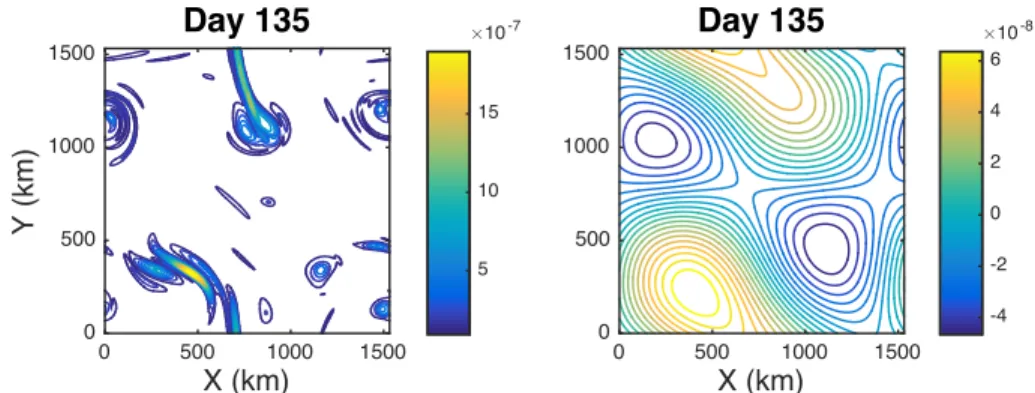
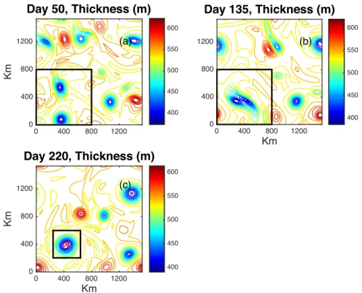
Our model consisted of a four layer f -plane fluid, with three subsurface interfaces, in a flat bottomed basin of 4,000 m of total depth. The free surface and third layer interface were initially taken as flat, and the second layer, bounded by the first and second interfaces, was seeded with an organized distribution of 200-m thick anomalies. All initial velocities were assumed to vanish. As expected, after a very short time adjustment involving gravity wave radiation, the fluid followed a classical path of like-signed vortex merger and opposite signed vortex propagation toward a final state of a single cyclonic-anticyclonic pair. Along the way, smaller vortices are swallowed by larger ones and a recognizable upscale energy cascade takes place. Examples of the fluid state at Days 50, 135, and 220 in Year 2 of the simulation appear in Figure 3 in which this sequence is evident.
Numerical details of the simulation appear in Table 1; here, we emphasize that the resulting internal defor-mation radii, 34, 19, and 14 km, are representative of the open ocean. The experiment was simulation for a total of 4 years, from which we focus on the analysis of Days 50–220 from the second year of the simulation. The sequence in Figure 3 comes from that interval, and we have focussed our attention on the merger event occurring in the lower, left-hand quadrant outlined by the black lines in the upper two panels. Qualitatively, the two vortices near the bottom of panel (a) on Day 50, with radial length scales of roughly 100 km, merge into the single, larger vortex seen in panel (c) at Day 220. The smaller square in panel (c) encloses the region over which averaging takes place (see Equation 33).
Figure 3. Three separate model states from a simulation of the MOM6 model with merging vortices. The top panels
are of second layer thickness at Days 50 (left) and 135 (right), and the bottom row shows Day 220. The quadrant enclosed by the heavy black lines in the upper panels contains two cyclonic vortices in the process of merger. The smaller square centered on the red “X” at Day 220 encloses the merged vortex and indicates the region over which the analysis takes place.
Closing budgets as we are attempting to do here requires high accuracy, especially in the solution of the adjoint equation. MOM6 does not have an adjoint option, so the following procedure was adopted. Output from the merger experiment of horizontal velocity components and thickness were cataloged at intervals of 1 day, from a simulation that used time steps of 300 s. The computational domain was doubly periodic and
f-plane, so we developed a spectral model for the adjoint equation in MATLAB. We adopted a comparable 300-s time step for the adjoint equation which, of course, required knowledge of the model state at
Table 1
Numerical Parameters and Values
Quantity Parameter Value
Zonal grid scale dx 4,000 m
Meridional grid scale dy 4,000 m
Time step dt 300 s
Zonal grid points nx 384
Meridional grid points ny 384
Coriolis parameter f 10−4s−1 Gravity g 9.8 m/s2 Layer 1 density 𝜌1 1,025 kg/m3 Layer 2 density 𝜌2 1,026.5 kg/m3 Layer 3 density 𝜌3 1,027.5 kg/m3 Layer 4 density 𝜌4 1,028 kg/m3 Total depth H 4,000 m Lateral viscosity 𝜈 40 m2/s
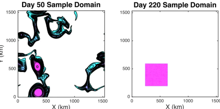
comparable temporal resolution. This was obtained for any given one 1-day interval by using 6 days of MOM6 data centered on that day to inter-polate via cubic splines the velocities and thickness to the required adjoint model times. The interpolated velocity and thickness data were used to compute kinetic energy and dissipation at the mass points of the model grid, and the pressure work at that point was estimated as the residual in the kinetic energy equation. Our estimates were checked against direct estimates of the pressure work which could be computed using the daily archived fields, and the two were found to agree to a high degree of accu-racy. In this way, we developed time series of the various inputs to the kinetic energy equation that balanced to machine precision, which in turn allowed us to balance our adjoint-based kinetic energy budgets. As is evident in Equation 37, the evolving modified Green's functions are related to Lagrangian measures of fluid displacement. This point is emphasized in Figure 4 which compares Green's functions correspond-ing to the beginncorrespond-ing and the end of our experiment, i.e., to Days 50 (left) and 220 (right). Comparatively speaking, the left-hand side looks con-siderably more disorganized than the right-hand side. This reflects the strongly interactive nature of the evolving fields, which moves particles
Figure 4. The modified Green's functions, defined by Equation 37, from our numerical experiment at Days 50 (left)
and 220 (right). The left panel essentially shows the distribution of the particles that end up in the square on the right. CI=.05e-4.
considerable distances. The distribution on the left represents the density of the particles over the entire domain on Day 50 that eventually, at Day 220, end up in the square on the right. The multiple maxima appearing on the left are indicative of the primary merging vortices that between Days 50 and 220 form the final vortex seen in Figure 3.
Fourteen different sampling functions,𝜋Li+1
Q,Li (see Equation 38), were developed, each designed to measure
the average kinetic energy contained in the region indicated in Figure 3 between two lengths, ranging from the full domain size (1,536 km) down to the grid scale. We used the first filter to remove the domain average, i.e.,
𝜋Lk
Q,L𝑗=1∕Ao (39)
where Lj=0 km, Lk=1,536 km, and Aois the domain area. Intermediate lengths were set to (L2→ L13) = 1,200, 1,000, 800, 700, 600, 500, 450, 400, 350, 300, 250, and 150 km. The adjoint problem appropriate to each of these sampling functions was solved to obtain fourteen different sets of ΦLi+1
Li functions, and the kinetic
energy, pressure work, and dissipation fields were filtered using each of the associated filtering functions. This resulted in a 14 × 14 matrix for each of the kinetic energy and energy input fields, detailing how the
Table 2
Band Numbers and Associated Length Scales
Band no Limits 1 Basin average 2 1,200–1536 km 3 1,000–1,200 km 4 800–1,000 km 5 700–800 km 6 600–700 km 7 500–600 km 8 450–500 km 9 400–450 km 10 350–400 km 11 300–350 km 12 350–300 km 12 300–350 km 13 250–300 km 13 150–250 km 14 0–150 km
various scale-dependent quantities contributed to the final kinetic energy at a given time. We will refer to the results in terms of the bands associated with the initial ΦLi+1
Li functions, as spelled out in Table 2.
For the purposes of this paper, we consider the transition from Days 50 to 220, i.e., over the entire interval of the vortex merger. We compare initial and final kinetic energy decompositions𝜅Li
o, where
𝜅Li
o = Σio𝜅 Li
Lo=0 (40)
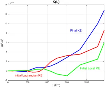
as functions of length scale in Figure 5. Note that some of the values are not positive. This is a consequence of Equation 17, which insures that when summed all filtered contributions converge on the value of the energy in physical space. What is guaranteed to be positive is the final sum. Contributions from individual length-scale bands can contribute negative values to achieve this goal.
The red line is𝜅Li
o of the initial kinetic energy within the square seen
in Figure 3c. Although relatively flat, it does exhibit a peak in the range
L =400–600 km which reflects the two vortices present at Day 50. While indicative of the early energy distribution, a more telling decomposition comes from that found by subsampling the field according to the Day 50 Green's function (see Figure 4). This appears in the green line, which
Figure 5. Initial length-scale structure of the kinetic energy,𝜅Li
o, compared
to final length-scale structure. The red line is based on the initial kinetic energy as sampled by the Lagrangian field in Figure 4 (left), the green line is based on the initial kinetic energy inside the square in Figure 4 (right), and the blue line is based on the final kinetic energy inside the square in Figure 4 (right). The final field (blue line) exhibits clear evidence of kinetic energy growth at longer scales.
shows a weak dip in values at small length scales, followed by a steady growth. The final, blue, line is the decomposition associated with the Day 220 state inside the square in Figure 3c. It is clear that, compared to both other curves, the kinetic energy has both grown considerably in amplitude, particularly at large L, which is consistent with an upscale cascade.
A more detailed view of the cross-scale exchanges is shown in Figure 6. Here, we plot the decomposition of the large-scale (Band 2), intermediate-scale (Band 8), and small-scale (Band 12) kinetic energy in the upper three panels. Each plot consists of 43 separate values. The first value is the band-passed kinetic energy at Day 220. This is followed in the next 14 slots by the initial kinetic energy contributions from the various bands. Those values are distinguished by a magenta axis. The next 14 slots are the various band-passed contributions from the pressure work (cyan axis), and the final 14 slots (blue axis) are the contributions from dissipation. Each group of 14 contributions is also separated by a vertical black line. The solid black horizontal lines in each slot are the values of the contributions, and the red line starting from the second slot shows the cumulative sum of the values. As shown in Equation 29, the sum of all the inputs should match the final band-passed kinetic energy; equivalently, the final red value at Slot 43 should match the black line in the first slot in amplitude. Note that this holds in all three plots. Finally, the three dashed green vertical lines mark the band corresponding to the band of the final kinetic energy for each of the initial kinetic energy, pressure work, and
Figure 6. Three kinetic energy decompositions corresponding to Bands 2 (upper), 8 (next upper), and 12 (next lower).
Vertical black lines limit the final kinetic energy in the band, the contributions to that band from the 14 bands of the initial kinetic energy, pressure work, and dissipation, respectively. Horizontal black lines denote values of the quantity, and the red line is the cumulative sum, moving to the right, of the various contributions. The abscissa denotes band number, and the ordinate is energy in m2/s2. The bottom plot connects the band number on the y-axis to the length
Figure 7. The kinetic energy distributions in Layer 2 from our model run appear in the upper row (Days 50 [left] and
220 [right]). The kinetic energy transfer in Band 2 from Days 50 to 220 appears in the lower left, and the Day 220 kinetic energy content in Band 2 appears in the lower right.
dissipation. Bands left of the green line correspond to larger length scales and those to the right to shorter length scales.
The bottom panel connects the band number on the y-axis with the length-scale range of that band on the
x-axis.
3.1. Large Scales
For example, consider Figure 6a. The first slot is occupied by
𝜅L2 L1(x, to) = ∫ xo K(xo, to)𝜋 L2 Q,L1(x − xo)dxo (41)
which is Band 2 kinetic energy in the final state, with a value of roughly 5.5 × 10⁻³m2/s2. A plot of the
physical space structure of this quantity appears in Figure 7d. The kinetic energy field at Day 220 from which this filtered content is extracted appears above it in Figure 7b. The next 14 slots, from Slots 2 to 15, are occupied by ∫xo 𝜅(x, 0)Ln+1 Ln Φ L2 L1(x, 0, xo;to)dxo (42) where 𝜅(x, 0)Ln+1 Ln = ∫ x1 K(x1, 0)𝛾Ln+1 Ln (x − x1)dx1 (43)
is the initial kinetic energy content contained in band n (see Table 2). The dashed green line marks the third slot, which is the second band of the initial kinetic energy. This is the same band appearing in the first slot, and a physical space picture of this transfer term appears in Figure 7c. Day 50 kinetic energy field from which this term is extracted by Equation 42 appears above it in Figure 7a. It is clear from comparing the black line in the green dashed slot to the black line in the first slot from Figure 6a that this band has grown in kinetic energy over the experiment, from an initial value of 1.3 × 10⁻³m2/s2to roughly 5.5 × 10⁻³m2/s2. The values
Figure 8. The distribution of dissipation at Day 135 appears on the left. Note that it is concentrated into small areas.
Dissipation as it affects Band 2 appears on the right. Although this is a large-scale mode, dissipation is still a major input to the kinetic energy development, as seen in Figure 6.
the initial kinetic energy to Band 2 final kinetic energy structure. The next four values in the initial kinetic energy zone are positive, indicating a transfer of smaller scales upward. The remaining slots are filled with very small values. The cumulative red line indicates the total transfer to Band 2 final kinetic energy from initial kinetic energy is roughly 3.3 × 10⁻³m2/s2, with the biggest single contributor being local Band 2. In
summary, this plot suggests an upscale kinetic energy to kinetic energy cascade. The slots from 16 to 29 are occupied by
∫ to o ∫x (−pw(x, t)Ln+1 Ln )Φ L2 L1(x, t, xo;to)dxodt (44) where pw(x, t)Ln+1 Ln = ∫ x1 (upx+vp𝑦)(x1, t)𝛾 Ln+1 Ln (x − x1)dx1 (45)
is the pressure work performed in band n at time t of the calculation. The green dashed line falls in Slot 17 because that band corresponds to the band appearing in the first slot. The values in the remaining slots represent contributions to Band 2 final kinetic energy from other bands in the pressure work occurring along the fluid trajectory. As can be seen from the red lines, pressure work is considerably more active across the bands than kinetic energy. The green dashed slot contains a negative value, indicating a net loss of kinetic energy by the pressure work in this band. However the next several slots are positive, indicative of an upscale cascade of energy due to pressure work, and in total, these transfers are considerably stronger than the in-band loss. In total, pressure work elevates kinetic energy by 3.8 × 10⁻³m2/s2and is roughly 3–4 times
larger than the kinetic to kinetic transfer, with most of the transfers coming from smaller scales. This result is somewhat surprising, as most previous studies have focussed on kinetic to kinetic transfers. Contributions from other sources, such as pressure work, have not received as much attention. Here, they are dominant. Last, we come to the dissipative contributions, appearing in Slots 30–43. Here, the surprise is that the net dissipative effects acting on Band 2 are relatively large. Over all scales, the net effect is slightly less than −1.3 × 10⁻³m2/s2, although the total is dominated by the in-band, Band 2, dissipative impact of slightly
more than −1.3 × 10⁻³m2/s2. The reason this is unexpected is that Band 2, from 1,536 to 1,200 km, is a
large-scale band, and dissipation is dominantly a small-scale process. This is certainly true as well in the present simulation, as is seen in Figure 8a of the modeled dissipation field at Day 135. However, dissipation is broadly distributed and occurs at locations governed by the large scale, so that when filtered, dissipation imprints importantly on the evolution. This appears in Figure 8b which is the dissipation field at Day 135 filtered through Band 2.
3.2. Intermediate and Small Scales
Band 8, in Figure 6b, loses kinetic energy over the simulation, as can be seen by comparing the black line in the first slot with that in the first green dashed slot. However, the scale of this loss is close to two orders of magnitude smaller than those described for Band 2. Essentially, this is an inert band in regard to kinetic to kinetic exchanges. Across the bands, initial kinetic inputs to final kinetic energy are quite small, at a
Figure 9. Time series of the pressure work input to kinetic energy. The pressure effect on Band 2 of Band 2 appears on
the left and on Band 2 due to Band 3 on the right. Note the difference in scale on the y-axis. The net pressure work between these two cases is opposite, with the Band 3 to Band 2 case leveling off late in the event, while the Band 2 to Band 2 case continues to drain kinetic energy.
net value of 3 × 10⁻⁶m2/s2. Note however that pressure work is quite active across all bands. Larger scale
bands, to the left of the green dashed line in the pressure work zone, tend to be positive. This is indicative of a down-scale transfer of energy from larger scales to Band 8. However, smaller scales tend to be negative in amplitude and overall comparable in size to the contributions from the larger scales. The net effect of pressure work across all bands is negative, at a value of −1.7 × 10⁻⁵m2/s2, indicative of a net transfer to
small scales. Band 8, with respect to pressure work, acts like a pass-through, allowing energy from larger scales to move through to smaller scales, while adding a small amount to the net. In this intermediate-scale band, the principal signal is a down-scale contribution to kinetic energy.
Finally, Band 12, in Figure 6c, is also a band of relatively weak energy transfers, if still stronger than Band 8. Overall, there is a stronger kinetic energy loss at these small scales, roughly −5.5 × 10⁻⁵m2/s2, most of
which, −4.0 × 10⁻⁵m2/s2is accounted for by losses to larger length scales. This is indicative of a kinetic to
kinetic upscale transfer. Once again, it is seen that the pressure work to kinetic energy transfers is far more active. While the net effect is relatively small, −1 × 10⁻⁵m2/s2, it is the result of large transfers of both signs
across the length-scale spectrum. A clear pattern does not emerge. Losses and gains to other length-scale bands of both larger and small character occur. Perhaps the safest interpretation is that the weak values involved in this band indicate that it responds erratically to the conditions imposed on it by the energetically dominant larger length scales.
Time histories of two of the pressure work energy transfers is shown in Figure 9, i.e., those for Band 2 to Band 2 and for Band 3 to Band 2. These are among the most active pressure work bands seen in Figure 6and, despite their similarity in length scales, show opposite trends. The Band 2 to Band 2 transfer appears on the left. Early in the experiment, pressure work adds to kinetic energy, but the trends reverses around Day 120, and pressure work depletes kinetic energy strongly to Day 220. The last 100 days are thus associated with a large-scale tendency for flow to be directed toward high pressures and away from low pressures. Figure 9b, the pressure work contribution of Bands 3 and 2, shows the opposite trend. Pressure work persistently builds kinetic energy through most of the experiment, except for the period from Days 100 to 120. Toward the end, the net levels to a constant value, equivalent to the cessation of pressure work contributions between bands.
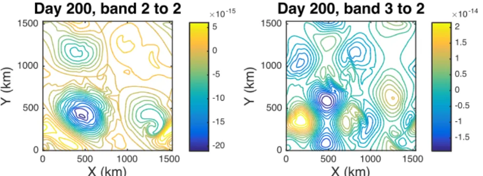
Figure 10. The anatomy of the pressure work occurring at Day 200, relatively late in the merger event. The pressure
effect on Band 2 of Band 2 appears on the left and from Band 3 to Band 2 on the right. The former case is dominated by negative values near regions of cyclones and reflects the tendencies at these largest scales for cyclones to merge. The distribution on the right-hand side is much more evenly distributed between positive and negative values and indicates a weaker pressure work associated with a more symmetrized, smaller scale structure.
These tendencies are explained in part by examining the anatomy of the pressure work contributions. For this, we show in Figure 10 the pressure work field as it appears to Band 2 at Day 200, for Bands 2 and 3. On the left is the pressure work as seen by Band 2, having been filtered through Band 2. Note that the structure is dominated by relatively large-scale negative values. These are zones dominated by cyclones and hence low pressures. The negative pressure work values indicate flows away from the low-pressure centers, which is a flow field designed to bring the lows together. As a result, the negative pressure work at largest scales is a signal of vortex merger. In contrast, the pressure work filtered through Band 3 as it appears to Band 2 appears on the right. Here, the distribution consists much more evenly of both highs and lows of comparable magnitude. Day 200 is relatively late in the merger event and is a point where on these scales of Band 3; the fields are becoming relatively symmetrized. As a result, the net pressure work from this band is quite small, consistent with the late parts of the time series in Figure 9 (right), where the time history of integrated pressure work has leveled off.
4. Summary
A new method for computing cross-scale energy transfers in fluid flows has been described and applied to a well-known example. The technique has both Lagrangian and Eulerian forms. In this paper, we mostly examine the former method, which exploits the Lagrangian nature of kinetic energy evolution to relate kinetic energy at any one location and time to its flow history. The Lagrangian history is computed by solving an adjoint equation obtained by a classical Green's function approach. The scale content of the final kinetic energy structure can be obtained by solving a filtered version of the adjoint equation and projecting the kinetic energy field onto the result. In addition, the same filter used on Green's function equation can be used to diagnose the scale-dependent inputs to the kinetic energy evolution, such as pressure work and dissipation, in a relatively straightforward way. This leads rather naturally to a quantification of how energy from one band of length scales transfers to another during the nonlinear evolution of the flow. The procedure also allows for a diagnosis of the nature of the energy transfers, e.g., kinetic to kinetic or kinetic to pressure work, as well as examination of how the transfers are structured in time and space. While we have here focussed on kinetic energy, the same approach can be applied to potential energy evolution.
We have applied the procedure to the classic problem of vortex merger in a stratified fluid. The well-known MOM6 model was deployed in a four layer isopycnal configuration and with an initial condition consisting of a sequence of undulations in second layer thickness. The system evolution proceeds with like-signed vortices merging and opposite-signed vortices pairing up and propagating. We analyzed a particular merger event in detail.
The subsequent analysis showed the expected result that kinetic energy exhibits an upscale cascade; how-ever, the procedure also illustrates several somewhat novel aspects about merger. Perhaps most significantly, the primary energy transfers involve pressure work to kinetic energy exchanges, rather than kinetic to kinetic energy exchanges. This result complements several published studies of upscale energy transfers which have focussed on Fourier transforms of the nonlinear advection terms in the momentum equations by
emphasizing the role played by pressure work. Dissipation also emerged as a surprisingly large effect on larger scale energy exchanges. This was due in part to the tendency for the larger scale flow to organize regions of small-scale dissipation so that the large-scale projection of dissipation was substantial. Also, sev-eral of the intermediate ranges in an integral sense were relatively inert, in that initial and final kinetic energies were often quite similar; however, those same ranges were found to be very dynamically active and acted as pass-throughs, receiving potential energy from smaller scales and passing them along to larger scales. Finally, the diagnoses identify the critical points in time when exchanges are at their peak and allows for an examination of the events associated with the exchanges. Spatial information about the nature of the exchanges is also provided and allows for a diagnosis of the involved mechanisms.
The example problem considered here is highly idealized, with an isotropic setting, doubly periodic bound-aries and an unobstructed geometry. The promise of the technique, however, is that it potentially generalizes in a straightforward way to realistic ocean simulations, in which the flows are highly anisotropic and inho-mogeneous, and the domains are often geometrically complex. The examination of such regions, such as the Gulf Stream, the Kuroshio, and other major ocean currents, is of importance to the understanding of the global ocean energy cycle. It will be of great interest to see what new light this method might cast on such regions.
Appendix A: Basis Functions for Arbitrary Domains
Trigonometric functions form the obvious filtering basis set for unbounded and simple domains. Unfor-tunately, such domains are rarely associated with realistic problems, so it is necessary to consider a generalization when filtering a variable in a realistic setting. The purpose of this appendix is to suggest one method to develop an appropriate basis set. We stress that the example in the main part of the paper uses classical trigonometric functions and does not involve any of the more elaborate filters computed here. The key property of trigonometric functions that leads to their utility is Equation 18. In turn, the demon-stration of this property for trigonometric functions depends on their orthonormality, i.e., that
∫
∞ −∞
𝑓n(x)𝑓m(x)dx =𝛿n,m (A1)
where fn(x) and fm(x) are two trigonometric functions characterized by eigenvalues n and m and𝛿n, mis the
Kronecker delta function. We wish to retain these properties while developing basis functions appropriate to more general settings.
It is widely recognized that orthonormal functions are often developed from dynamical equations. Here, we make the conscious decision to avoid any basis set developed from dynamical considerations. The reason for this is we want to make a scale-dependent statement only and not a statement about any preconceived dynamical content. To this end, consider the classical Helmholtz equation
∇2𝜓 + k2𝜓 = 0 (A2) In the presence of homogeneous boundary conditions, the solution of this equation is𝜓 = 0, except possi-bly for special values of the constant k, making it an eigenvalue problem. By construction, the eigenvectors of Equation A2 are the eigenvectors of the Laplacian operator. If one is in possession of two separate eigen-vectors of Equation A2, say𝜓mand𝜓n, they are automatically orthogonal, as we now demonstrate. First,
insert one of these eigenvectors into Equation A2 and multiply by the other
𝜓n∇2𝜓m+𝜓nk2m𝜓m=0 (A3)
where kmis the eigenvalue associated with𝜓m. Integrating over the domain in question
∫S
(𝜓n∇𝜓m−𝜓m∇𝜓n) + ∫
V
(𝜓m∇2𝜓n+𝜓mk2
m𝜓n)dV =0 (A4)
where S is the domain boundary enclosing the integration volume V . In the presence of homogeneous boundary conditions and introducing the remaining eigenvalue kn
(k2 m−k 2 n)∫ V𝜓m𝜓n dV =0 (A5)
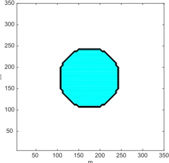
Figure A1. An example of an irregular domain, consisting of a circular
island inside a square domain. The island, outlined in black, occupies about 10% of the area. Vanishing boundary conditions are put on the island boundary and periodic conditions on the outer edge.
Equation A2 being a Sturm-Liouville equation possesses an infinity of eigenvector/eigenvalue pairs that can be ordered from smallest to largest, so, in general, the factor multiplying the integral on the left-hand side of Equation A5 does not vanish. Thus, by construction, the eigenvalues are orthogonal. Enforcing
∫V
𝜓2
mdV =1 (A6)
insures they are also suitably normalized. Further classical analysis shows that arbitrary functions in V can be represented by an appropriate superposition of the eigenfunctions (in a least-squares sense) where the coefficients of the representation are computed by exploiting orthonor-mality.
In regard to the length scale, L, we would associate with any particular eigenfunction; the form of the Helmholtz equation suggests
L ≈ k−1 (A7)
We will see in multiple dimensions that this simple relationship is prob-lematic.
While for irregular domains with islands and topography, the solutions cannot generally be written down, they can be developed in relatively straightforward numerical ways. As an example, consider the domain shown in Figure A1, consisting of a single circular island inside of an otherwise square domain. The Laplacian operator is discretized using a 5-point stencil. Periodic boundary conditions are placed on the outer edge of the domain, and the eigenfunctions are required to vanish on the island boundary. These are conditions consistent with the orthogonality of the resulting Helmholtz solutions and are entirely reflected in the details of the stencil coefficients. In principle, the coefficients can be formed into a nx × ny by nx × ny square matrix, where nx and ny are the lengths of the domain in the east-west, north-south directions, respectively. For the present calculation, nx = n𝑦 = 70 and grid spacing dx, d𝑦 = 5m is isotropic. In fact, this does not account for the island, inside of which are several of the regularly spaced grid points but which represent locations inaccessible to the fluid. It is necessary to remove those points, resulting in slightly smaller matrix, the regular, pentadiagonal structure of which is then interrupted. This matrix can be fed into a standard eigenvalue extraction routine; we used the function “eig” in MATLAB. The gravest and 10th-most gravest eigenmodes appear in Figure A2; these are associated with eigenvalues
k2 1≈10
−4m−2on the left and k2
10≈1.4 × 10
−3m−2, or equivalently L
k≈200 m (left) and L10≈52 m (right). It
is easy to associate a length scale of 200 m with the former, but the latter also measures comparable length scales while being spatially considerably more complex. It is thus not straightforward to simply connect the eigenvalue size and the associated length scale. This is due to the multiple spatial dimensions involved in the
Figure A2. The first (left) and tenth (right) eigenmodes of the Helmholtz equation for the domain in Figure A1. The
island location appears in black. Clearly, the gravest mode captures the broadest possible scales of the domain and can be associated with the length scaleL =200 m. The higher mode, however, while more complex spatially, is also measuring comparable length scales of roughly 200 m, in spite of being associated with a much higher eigenvalue.
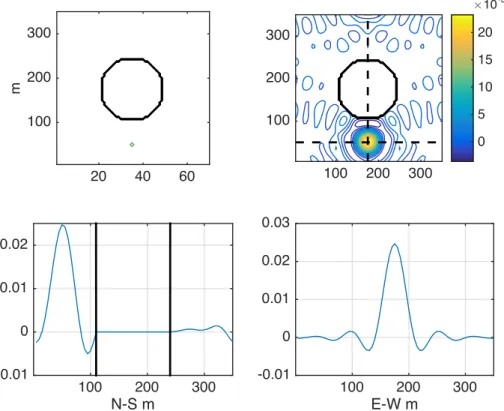
Figure A3. (Top left) The reconstruction of a Dirac delta function inside the domain in Figure A1. The island location
appears in black (in all panels), and the delta function appears just to the south of mid island. Theγ100sampling
function (top right). Note that it does not penetrate the island, instead sampling only the active fluid. The dashed black lines denote the locations of the transects appearing in the lower panels. The north-south transect throughγ100appears
on the lower left. The black lines denote the island location at this longitude. The east-west transect throughγ100
appears lower right. Note the qualitative resemblance of the structure to a sinc function. The distance between neighboring high lobes is roughly 75 m and consistent with the rough length-scale estimate of 90 m associated with the eigenvalue.
analysis and arises in the unbounded domain using simple trigonometric functions as well. For example, high wavenumbers in the meridional direction coupled to low wavenumbers in the zonal direction can be associated with eigenvalues very similar to comparable wavenumbers of intermediate values distributed symmetrically in the two directions. We recommend a different way to associate length scales to the analysis below.
We now demonstrate that these functions satisfy constraint (Equation 18). Exploiting orthonormality, we anticipate ∑ n an𝜓n(x) =𝛿(x − xo) (A8) where an=𝜓n(xo) (A9)
The result of evaluating this formula using the present eigenfunctions appears in Figure A3 (top left), where the source point xo=50 and 150 m, i.e., just south of the island. Clearly, we have reproduced to within
domain discretization a Dirac delta function. The analysis in the main part of the paper, however, empha-sized the use of integrals of filters between two length scales. We present in Figure A3 (top right) the result of summing all the eigenfunctions below a given eigenvalue. This corresponds to Equation 28, in particular to𝛾oL𝑗for the 100th eigenvalue (k2100≈.012). Cross sections of the sampling function on the dashed lines in
Figure A3b appear in the two lower panels. Note that the sampling function𝛾100avoids the island, as seen
in Figure A3 (bottom left), while maintaining a qualitative resemblance to the sinc function (Figure A3, bot-tom right). The length scale L associated with the eigenvalue is roughly 90 m, which corresponds well to the

![Figure 7. The kinetic energy distributions in Layer 2 from our model run appear in the upper row (Days 50 [left] and 220 [right])](https://thumb-eu.123doks.com/thumbv2/123doknet/13778742.439509/14.918.315.813.132.532/figure-kinetic-energy-distributions-layer-model-appear-upper.webp)