HAL Id: hal-01522004
https://hal.archives-ouvertes.fr/hal-01522004
Submitted on 12 May 2017
HAL is a multi-disciplinary open access
archive for the deposit and dissemination of
sci-entific research documents, whether they are
pub-lished or not. The documents may come from
teaching and research institutions in France or
abroad, or from public or private research centers.
L’archive ouverte pluridisciplinaire HAL, est
destinée au dépôt et à la diffusion de documents
scientifiques de niveau recherche, publiés ou non,
émanant des établissements d’enseignement et de
recherche français ou étrangers, des laboratoires
publics ou privés.
Aboveground Biomass Estimations From ICESat/GLAS
Data in Eucalyptus Plantations in Brazil
Nicolas Baghdadi, Guerric Le Maire, Ibrahim Fayad, Jean-Stéphane Bailly,
Yann Nouvellon, Cristiane Lemos, Rodrigo Hakamada
To cite this version:
Nicolas Baghdadi, Guerric Le Maire, Ibrahim Fayad, Jean-Stéphane Bailly, Yann Nouvellon, et
al..
Testing Different Methods of Forest Height and Aboveground Biomass Estimations From
ICESat/GLAS Data in Eucalyptus Plantations in Brazil.
IEEE Journal of Selected Topics in
Applied Earth Observations and Remote Sensing, IEEE, 2014, 7 (1), pp.290-299.
D
Testing Different Methods of Forest Height
and Aboveground Biomass Estimations From
ICESat/GLAS Data in Eucalyptus
Plantations in Brazil
Nicolas Baghdadi, Guerric le Maire, Ibrahim Fayad, Jean Stéphane Bailly, Yann Nouvellon, Cristiane Lemos, and
Rodrigo Hakamada
I. INTRODUCTION
ATA acquired by the Geoscience Laser Altimeter System (GLAS) on board the Ice, Cloud, and Land Eleva- tion Satellite (ICESat) between 2003 and 2009 have been successfully used to estimate tree heights and aboveground forest biomass (e.g., [1]–[13]). GLAS 1064-nm waveforms correspond to backscatter energy as a function of time. They are digitized in 544 or 1000 bins with a bin size of 1 ns for land (15 cm vertical resolution), corresponding to 81.6 and 150 m height ranges, respectively. The GLAS laser footprints have a near circular shape of about 60 m in diameter and a footprint spacing of about 170 m along the track. For forest applications, the data used consist of the GLA01 and GLA14 products. These products provide the full received waveforms and the land surface elevation data, respectively [14]. The horizontal geolocation error of the ground footprints is lower than 5 m on average for all ICESat missions, and lower than 5 m in standard deviation, except for the L2C, L2D L2E, and L2F missions, where the standard deviation is between 7.4 and 15.6 m for L2D and L2F missions, respectively [14]. The vertical geolocation accuracy ranges between 0 and 3.2 cm on average with a standard deviation under 3.3 cm for all missions except for the L2C, L2D, L2E, and L2F missions (between 5.1 and 10.9 cm) [14].
The accuracy obtained on the forest height estimates in numerous studies using the GLAS data has varied between 2 and 10 m according to the forest type and the characteristics of the study site (mainly the topography of the terrain) (e.g., [3]–[5], [7], [8], [10], [11], and [13]). GLAS data are often used together with auxiliary datasets to estimate aboveground biomass. The auxiliary data is mainly composed of airborne laser data, a digital elevation model, and optical and radar images. The recent paper by Saatchi et al. [12] provides the spatial distribution of aboveground forest biomass in tropical regions over three continents (Latin America, sub-Saharan Africa, and Southeast Asia) using GLAS, MODIS, QSCAT (spaceborne scatterometers at 12 GHz), the SRTM digital elevation model, and ground data with an overall accuracy of 23.8%. Using only the forest height estimated from GLAS data, Lefsky et al. [6] obtained a biomass estimate accuracy of 58.3 Mg/ha for biomass values lower than 350 Mg/ha. Nelson
et al. [9] estimated Siberian timber volume using MODIS and
However, three main limitations have been pointed out by re- searchers: 1) the low density of the GLAS footprint count and the lack of data over wide areas of the world; 2) the high sensi- tivity of GLAS returns to terrain topography due to the large footprint size of GLAS impacts on forest height estimations [10]; 3) for denser and higher canopies, laser penetration is re- duced and, consequently, the ground return needed to estimate canopy height is not detectable or has a low intensity.
The objective of this paper was to test the best known models used for estimating canopy height using full waveform LiDAR data. Studies to estimate forest heights from LiDAR data have highlighted that the fitting coefficients of developed models are strongly dependent on environmental factors, such as the re- gion of the study site, terrain topography, and forest type. In this paper, we evaluate the main models developed to predict canopy height using a combination of parameters extracted from GLAS waveforms (GLA14 and GLA01 products) and a digital elevation model, in order to explore which combination of pa- rameters yields the best forest height estimates. In addition, a model to estimate aboveground biomass from dominant height was calibrated. Canopy height and aboveground biomass esti- mates derived from GLAS data were compared with inventory measurements.
A description of the dataset used in this study is given in Section II, followed by the presentation of methods for forest height and aboveground biomass estimations using ICESat/GLAS in Section III. The results are shown and dis- cussed in Section IV, and finally Section V presents the main conclusions.
Fig. 1. GLAS/ICESat tracks over our study site.
A. Study Area
II. DATASET DESCRIPTION
The study area was located in Brazil, ranging from 47 31’ to 47 38 longitude West and from 21 29 to 21 39 latitude South (Fig. 1). The area was mainly covered with industrial, fast-growing Eucalyptus plantations managed for pulpwood by the Internationnal Paper do Brasil company [15]. Seedlings or clones of E. grandis (W. Hill ex Maiden) x E. urophylla (S. T. Blake) hybrids were planted in rows at a density of approx- imately 1300 trees/ha and were being harvested every six to seven years, with very little tree mortality (under 7%). The an- nual productivity of the plantations depended on the growth stage, soil type, fertilization, climate, etc., but was generally above 30 m /ha/year, sometimes reaching values as high as 60 m /ha/year. At harvest time, the stand volume was there- fore about 250–300 m /ha, and the dominant height was about 20–30 m. These plantations were managed locally by stand units of variable area ( 50 ha on average for the studied stands). Management practices were uniform within each stand (e.g., harvesting and weeding dates, genetic material, soil prepara- tion, and fertilization). Chemical weeding was carried out in the first year after planting, resulting in a very sparse under- story and herbaceous strata in these plantations. A few Euca-
lyptus trees were dominated from the early growth stages and
remained small throughout the whole rotation, but their leaf area and biomass were very low compared with regular trees (see [16, Fig. 1]). The stands were therefore rather simply structured with a crown layer of 3 to 10 m in width above a “trunk layer” of 0 (in the first months) to 20 m in height (Fig. 2) with very few
Fig. 2. Eucalyptus stand during harvest illustrating the clearly separated crown and trunk strata (dominant height of 30 m).
understories. In the study area, the stands were established in a low to moderate topographic relief (slope under 7 ).
B. In Situ Measurements
A total of 114 Eucalyptus stands were selected, corre- sponding to the stands where GLAS footprints were totally included, with an additional 10-m buffer strip from the stand borders to account for any footprint geolocation errors. This selection was also intended to avoid mixing effects within a GLAS footprint. In these 114 Eucalyptus stands, two to eight permanent inventory plots were measured regularly by the company between November 2002 and May 2009. During a rotation, three inventories were generally carried out: around the age of two years, four years, and before harvesting (approximately six years). Permanent inventory plots had an area of approximately 400 to 600 m and were systematically
TABLE I
THE NUMBER OF EXPLOITABLE ICESAT FOOTPRINTS FOR EACH YEAR. OF THE 1387 FOOTPRINTS
ACQUIRED OVER OUR STUDY SITE, THE NUMBER OF USABLE SHOTS WAS 800
Fig. 3. Dominant height calculated on the ICESat footprint acquisi- tion date using neighboring data (linear interpolation of measured on inventory plots in the stand including ICESat footprint).
distributed throughout the stand with a density of one plot per 12 ha. They included 30 to 100 trees (average of 58 trees). During a field inventory, the diameter at breast height (DBH, 1.3 m above the ground) of each tree in the inventory plot, the height of a central subsample of 10 trees, and the height of the 10% of largest DBH (dominant trees) were measured. The mean height of the 10% of the largest trees defined the domi- nant height of the plot , while the mean height of the 10 central trees defined the average height of the plot . The , basal area, and age on the inventory date were then used in a company-calibrated volume equation, specific to the genetic material, to estimate the plot stem volume (wood and bark of the merchantable part of the stem that has a diameter of more than 2 cm). Trunk biomass was then estimated from the trunk volume using age-dependent estimates of wood biomass density (see [17] for more details). Plot-scale and biomass were then averaged on a stand scale, for each inventory date.
As the dates of the ground measurements were different from the GLAS acquisition dates, plantation dominant height and stem biomass for the GLAS acquisition dates were estimated using linear interpolations of the inventory plot measurements between the two dates either side of each GLAS acquisition date (Fig. 3). This simple linear interpolation gave fairly good esti- mates since forest inventories were regularly carried out.
Note that these estimates of and biomass gave a large and unique dataset for testing methods of height estimations from GLAS data since the measurements of these variables is precise compared to natural forests: uniform stands with rela- tively low dispersion of tree sizes around the average values, accurate allometric equations, large number of inventory plots within a stand, short intervals ( years) between inventory dates, a relatively gentle slope, and a simple canopy with a
Fig. 4. Typical GLAS waveform acquired over a forest stand, on relatively flat terrain, and the associated main metrics (1 15 cm).
clearly separated crown layer and the very sparse understory and herbaceous strata.
C. GLAS/ICESat Data
A dataset of LiDAR data acquired by the Geoscience Laser Altimeter System (GLAS) was used. In total, 1387 recorded signals (waveforms) were acquired over our study site between February 2003 and March 2009 (Table I, Fig. 1). Fig. 4 shows a typical waveform over a forest stand on relatively flat terrain. For our forest stands, the GLAS waveforms were generally bi- modal distributions resulting from scattering within the canopy and the ground surface. Of the 15 ICESat data products, only products GLA01 and GLA14 in release 33 were used in this research. For each ICESat footprint, these products provided a raw waveform, an acquisition date and time, the precise ge- olocation of the footprint center, waveform parameters derived from the Gaussian decomposition, the estimated noise level, i.e., the mean and standard deviation of background noise values in the waveform, etc. Each received waveform was decomposed into a maximum of six Gaussian functions corresponding to re- turns from different layers between the top of the forest and the ground. Over flat terrain, the first Gaussian corresponds to a reflection from the top of the canopy while the last Gaussian mostly refers to the lowest point in the footprint, i.e., the ground surface.
In order to use only the reliable ICESat data, several filters were applied to the waveforms to remove ICESat data contam- inated by the clouds and other atmospheric artefacts (e.g., [2], [4], [18]): 1) waveforms with ICESat centroid elevations signifi- cantly higher than the corresponding Shuttle Radar Topography Mission (SRTM) elevation (resolution of 90 m 90 m) were excluded ( ICESat-SRTM 100 m; 2) waveforms with low signal-to-noise ratios (SNR) were also removed SNR ; 3) saturated waveforms were removed (GLAS detector saturation index ); and 4) only the cloud-free waveforms were
kept cloud detection flag . FRir_qaFlag and satNdx are both indices recorded in the GLA14 product.
The application of different filters on the ICESat dataset showed that among the 1387 waveforms acquired over our study site, the number of usable waveforms respecting the filter condition was 800 (57.7% of waveforms), of which 306 had corresponding ground measurements.
For comparison between ICESat, SRTM DEM, and in situ data, datasets needed to be available in the same coordinate system. The ICESat ellipsoidal heights (TOPEX/Poseidon ellipsoid) were first transformed to the WGS84 ellipsoid by subtracting 70 cm, then orthometric heights from ICESat were derived with respect to the WGS84 reference system and the EGM96 geoid model.
III. MATERIALS AND METHODS
A. Forest Height Estimation
1) Direct Method: The most commonly used method to esti-
mate the maximum canopy height from a GLAS wave- form over forest stands with a gently sloping terrain uses the difference between the signal begin and the ground peak
[19]:
(1) The signal begin and the signal end correspond respectively to the highest and lowest detected surfaces within the laser foot- print. They are defined by the first and last bins at which the waveform intensity exceeds a certain threshold above the mean background noise. Different thresholds have been used in pre- vious studies. Their levels correspond to the mean background noise plus 3 to 4.5 times the standard deviation (3 times in Sun
et al. [20]; 3.5 times in Hilbert and Schmullius [4]; 4 times in
Lefsky et al. [6] and Xing et al. [13]; 4.5 times in Lefsky et al. [7]). Chen [2] examined several thresholds between 0.5 and 5 times the standard deviation. He demonstrated that the optimal threshold depends on the study site (between 3 and 4.5 times the standard deviation). The background noise statistics are avail- able in the GLA01 product.
The ground peak is assumed to be either the last peak (e.g., [3], [13], [20]) or one of the last two Gaussian peaks with the greatest amplitude (e.g., [4] and [11]). Harding and Carabajal [19] specify that, in the case of a low amplitude final peak, the better representation of the ground surface is probably the peak close to the last one with a relatively high amplitude. Chen [2] found for his conifer sites that the ground elevation corre- sponded better to the stronger peak of the last two, whereas for his woodland site the strongest peak of the last five matched best with the ground elevation.
2) Regression Models: Over sloping terrain, the ground peak
becomes wider, and the returns from ground and vegetation can be mixed in the case of large footprints, making the identifica- tion of ground peak returns difficult and the estimation of forest height inaccurate [6], [19]. To remove or minimize the terrain slope effect on the waveforms, statistical approaches have been developed and used in several studies to predict canopy height
waveform metrics or on both waveform metrics and terrain in- formation derived from DEMs.
The main waveform metrics used in these models are the waveform extent defined as the height difference between the signal begin and the signal end of a waveform ( , in meters), the leading edge extent ( , in meters) calculated as the elevation difference between the elevation of the signal begin and the first elevation that is at half maximum intensity above the background noise value (highest detectable return), and the trailing edge extent ( , in meters) determined as the dif- ference between the signal end and the lowest bin at which the waveform is half of the maximum intensity (lowest detectable return) [7] (Fig. 4).
The terrain information used in the regression models is the terrain index ( , in meters) derived from a DEM (from SRTM or airborne sensors). is defined as the difference between maximum and minimum terrain elevations in a given window centered on each GLAS footprint. The size of the window which depends on the spatial resolution of the DEM is generally 7 7 for a 10-m resolution DEM (airborne) and 3 3 for a 90-m res- olution DEM (SRTM) (e.g., [6], [7], and [11]).
The first statistical model was developed by Lefsky et al. [6] to estimate the maximum canopy height from GLAS waveforms:
(2) This model is based on the waveform extent and terrain index calculated from a high quality DEM. The coefficients and are fitted using least squares regression given by ground measurements or estimated from airborne LiDAR data, is derived from the GLAS waveform, and is calculated from the DEM). For our data set, values were calculated from SRTM DEM range from 0 and 40 m. The incorporation by Lefsky et
al. [6] of the waveform leading edge extent in the (2) shows a
slight improvement in canopy height estimation:
(3) Xing et al. [13] observed a logarithmic behavior between the canopy height and the waveform extent. Thus, they proposed an adapted version of Lefsky’s model:
(4) Lefsky et al. [7] and Pang et al. [10] proposed regression models with metrics derived only from waveforms. Lefsky et
al. [7] observed that on sloping terrain, the waveform extent is
insufficient for estimating canopy height. Hence, a new model based on the waveform extent, leading edge extent, and trailing edge extent was proposed. However, Pang et al. [10] observed inaccurate estimates of canopy heights with this new Lefsky model, especially for small waveform extents, and thus pro- posed a simpler model to estimate canopy height using the fol- lowing equation:
(5) Chen [2] proposed a linear model from Pang’s nonlinear model (5):
from GLAS data (e.g., [2], [6], [7], [10], [11], and [13]). These
Fig. 5. Leading edge and trailing edge compared to modified leading edge and modified trailing edge according to Hilbert and Schmullius (2012).
Lefsky [8] proposed a modification of Lefsky’s 2007 model for a better estimation when the leading and trailing edges are small:
(7) where and correspond to the tenth percentile of waveform energy.
The fitting coefficients of each of these different statistical models (they differ from one model to another) are de- pendent on vegetation type and terrain topographic conditions, and it is therefore necessary to recalibrate them ([2], [7], [10]).
Hilbert and Schmullius [4] proposed a modified leading edge and trailing edge. The first new metric is defined as the ele- vation difference between signal begin and the canopy peak’s center, and the second metric as the difference between signal end and the ground peak’s center (Fig. 4). These modified met- rics more effectively represent the characteristics of the top of the canopy and the ground surface, especially for waveforms with a large difference in the intensity between the canopy and ground peaks. The results show that in the case of a low in- tensity return from the ground peak and a high intensity return from the canopy peak, an overestimation of the trailing edge might be observed using Lefsky’s metrics. For a low-intensity return from the canopy peak and a high-intensity return from the ground peak, an overestimation of the leading edge might be observed using Lefsky’s metrics (Fig. 5). In this study, the modified leading and trailing edges were used.
The different regression models defined in equations (2)–(7) to estimate forest height were evaluated in this work, except for (7) where and were replaced by
and , respectively. In fact, Lefsky [8] proposed using and instead of, and in order to obtain, a more stable regression model between the canopy height and the waveform metrics. The use in this study of, and as defined by, Hilbert and Schmullius [4] makes the use of and unjustified (Hilbert and Schmullius [4] metrics are more stable than those defined in Lefsky [8]).
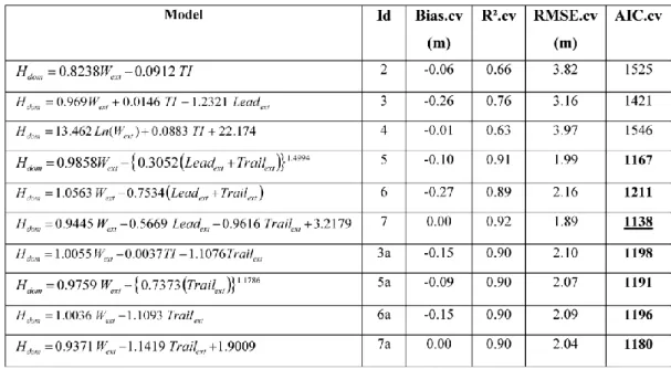
In addition, to quantify the contribution of and in the height estimation models, four other models were analyzed: model 3 by replacing by , and models 5, 6, and 7 by removing (Table II). The best regression model was selected from the set of these ten models using the Akaike information criterion (AIC), the mean difference between the forest height predicted from GLAS and DEM metrics and the measured forest height (Bias), the coefficient of determination , and the root mean-square error (RMSE). The Akaike information criterion proposed by Akaike [21] is a measurement of the relative goodness of fit of a statistical model to the truth. By calculating AIC values for each model, the acceptable regression models based on lowest AIC values were identified. Indeed, the best model is the one that minimizes the Kullback–Leibler distance between the model and the truth. In this analysis, a tenfold cross validation with ten replications was used. Lower AIC values indicate model parsimony, i.e., a balance between model performance (explained variability) and coefficient number in the model.
B. Aboveground Biomass Estimation
Several studies have shown that forest canopy metrics cal- culated from GLAS waveforms can be used to estimate above- ground biomass [1], [6], [12]. Lefsky et al. [6] proposed a linear relationship between the aboveground biomass ( in Mg/Ha) and the forest maximum height squared (height is in me- ters):
(8) Boudreau et al. [1] developed a model to estimate for the entire forested region of the Province of Quebec, based on wave- form extent (in meters), terrain index (in meters), and the slope between signal begin and the first Gaussian canopy peak ( in radians):
(9) The slope depends on the canopy density and the vertical variability of the upper canopy. For a given study site with only a few variations in and , the biomass in Boudreau’s model follows a second-order polynomial relationship with the forest height because the waveform extent is expressed in Fig. 6(a) as proportional to .
Saatchi et al. [12] used a power law relationship between the aboveground biomass and Lorey’s height, calibrated on in situ forest plots and GLAS data collected over Latin America, sub- Saharan Africa and Southeast Asia:
(10) where is Lorey’s height, which weights the contribution of trees (all trees 10 cm in diameter) to the stand height by their basal area. The mean exponent of the combined relation from
TABLE II
REGRESSION MODEL FITTING STATISTICS CALCULATED WITH TEN-FOLD CROSS VALIDATION FOR ESTIMATING FOREST HEIGHT. ROOT MEAN-SQUARE ERROR,
AKAIKE INFORMATION CRITERION, CROSS VALIDATION
the three continents is near 2.02 (with ) [12]. In this study, the relationship defined in (10) was used by replacing Lorey’s height with the dominant height . In- deed, in these Eucalyptus plantations, Lorey’s height was very close to dominant height ( was lower than by a max- imum of 0.9 m at the end of the rotation of the Eucalyptus plan- tation). To illustrate this, Fig. 7 shows the evolution of the dif- ferent stand height metrics on an experimental stand during a full rotation (height data of the Eucalyptus monoculture treat- ment described in [22]). Note also that the crown area weighted version of Lorey’s height gives values very close to [10].
The coefficients and were fitted using the in situ measure- ments of dominant height and aboveground biomass. The fitted coefficients ( and ) were used to estimate the biomass, based on the dominant height predicted from GLAS footprints by the direct method (model 1).
IV. RESULTS AND DISCUSSIONS
A. Forest Height Estimation
First, both the optimum threshold levels above the mean background noise and the most relevant location of the ground peak that gave the best estimates of canopy heights were determined. The two thresholds of 3.5 and 4.5 times the noise standard deviation were evaluated, and the ground peak was derived from the Gaussian with the higher amplitude of the last two. The difference between the canopy height estimated from GLAS waveforms using the direct method and in situ measurements showed better results with a noise threshold of 4.5 and when choosing the Gaussian with the greater amplitude of the last two as the ground peak. The bias and standard devi- ation of the difference between dominant height estimates and measurements decreased from 2 to 1.5 m when the Gaussian with the higher amplitude of the last two was used as the ground return instead of the last one (Fig. 8). However, the results
were similar with thresholds of 3.5 and 4.5 (similar standard deviation but bias lower by 0.5 m with a threshold of 4.5). With the optimum configuration (threshold of 4.5 and the highest Gaussian), the mean difference between height estimates using the direct method (model 1) and in situ measurements was 0.33 m with a standard deviation of 2.2 m.
The regression models fitting the statistics calculated with tenfold cross validation for estimating forest height showed that the models using the trailing edge extent (models 5 to 7a, Table II) provided a good estimation of canopy height. For these models, RMSE cv (cross-validation RMSE) was between 1.89 m and 2.16 m, AIC cv (cross-validation AIC) was between 1138 and 1211, and (cross-validation
) was between 0.89 and 0.92. The best fitting results for estimating forest height were obtained with model 7 (lowest AIC cv and RMSE cv and highest values, 1138, 1.89 m, and 0.92, respectively). Fig. 9 compares the canopy height estimates obtained with model 7 in comparison to measured canopy heights (field measurements). The results also showed that the contribution of the leading edge extent in the regression models was weak for height estimation accuracy. Indeed, the fitting statistics obtained with models 5, 6, and 7 (including the leading edge extent) showed a slight improvement over those obtained with models 5a, 6a, and 7a (Table II). For example, RMSE cv was better than 15 cm at best when the leading edge extent was used. Hence, using the leading edge extent in the regression models was not necessarily justified.
Moreover, use of information in the model calibration cal- culated from an insufficiently accurate DEM (terrain index) led to poor estimation of the canopy height (models 2, 3, and 4) except for model 3a where the use of instead of led to good model fitting statistics (for model 3a, AIC cv and RMSE cv were 1198 and 2.10 m, respectively, instead of 1421 and 3.16 m for model 3). Models 2, 3, and 4 provided a lower (between 0.63 and 0.76), a higher
Fig. 6. Behavior of canopy height according to waveform extent, leading edge extent, trailing edge extent, and terrain index.
RMSE cv (between 3.16 and 3.97 m), and a higher AIC cv (between 1421 and 1546). The results also showed that the nonlinear form of model 5 did not appear to be justified because
Fig. 7. Comparison of three stand level height metrics in a Eucalyptus plan- tation experimental stand during a full rotation. Mean height is the arithmetic mean of all tree heights, dominant height is the height of the trees that have the highest basal area (8% biggest trees), and Lorey’s height is a basal area weighted average height.
Fig. 8. Comparison between canopy dominant height estimates and in situ measurements. The “highest Gauss” estimates use the Gaussian with the higher amplitude of the last two as the ground return while the “Last Gauss” estimates use the last Gaussian as the ground return. The threshold of 4.5 times the noise standard deviation was used. Both correspond to model 1 (direct method).
the observed improvements with this model in comparison to model 6 (linear form) were weak. Lastly, the logarithmic relation between canopy height and waveform extent did not appear to be relevant (model 4).
For our study site where the terrain was flat or slightly sloping (slope under 7 ), the results showed that the accuracy of the canopy height estimates was similar between the direct method and the best statistical models (RMSE about 2 m). Numerous studies using GLAS data over natural forest ecosystems have shown that the estimated forest height accuracy varied between 2 and 10 m (RMSE), depending on the forest type (tropical, boreal, temperate deciduous, temperate conifer, etc.) and the characteristics of the study site (mainly the terrain slope) (e.g., [3]–[5], [7], [8], [10], [11], and [13]). However, no studies using GLAS data (larger footprint LiDAR) were found in the literature over forests with intra-plot homogeneity similar to tree planta- tions (little variation in tree heights, same species, etc.), and well
Fig. 9. Canopy height estimates from model 7 in comparison to measured canopy height. Statistics are given in Table II.
documented (high quality in situ measurements of forest height and biomass), and with a gently sloping terrain.
The analysis of dependency between the in situ canopy height and the GLAS waveform extent showed a linear re- lationship between the two parameters with an of 0.66 [Fig. 6(a)]. The coefficient decreased with the trailing edge extent and leading edge extent (Hilbert Gauss) [Figs. 6(b) and (c)]. Linear relationships were found between and the trailing extent, leading extent, and the sum of trailing and leading ex- tents [Fig. 6(d)]. This analysis confirmed the great importance of the trailing edge extent in the regression models for canopy height estimations. The importance of the leading extent was lower ( 44% with leading, 75% with trailing, and 78% with both trailing and leading). Fig. 6(e) also shows that was almost constant with the terrain index for the TI values at our study site under 40 m.
B. Aboveground Biomass Estimation
Aboveground biomass estimation using the models defined in (8) and (10) was inferred from the forest height. In model 9, the biomass was defined as the forest height squared with the forest height defined as . This equation of forest height was close to that given in model 2 (Table II). However, in the previous section (Section IV-A), the different regression models for estimating forest height from waveforms and DEM metrics showed that the models using the terrain index (TI) gave the poorest accuracies (models 2, 3, 4). This is probably due to the resolution of the SRTM DEM used (90 m 90 m), which was not optimal for a study site with gentle terrain slopes. For this reason, only models 8 and 10 were evaluated for the biomass estimation using the forest height es- timated by the direct method.
The in situ measurements of forest height and aboveground biomass were not totally independent since was used in the calculation of tree volumes (Fig. 10, cf. Section II-B). The simple model of (10) ( was estimated by the direct method) gave a fairly good estimate of stand-scale
Fig. 10. Allometric relation between aboveground biomass and dominant forest height from in situ measurements (stand-scale biomass from stand-scale
).
Fig. 11. Comparison between estimated and measured biomass.
biomass from stand-scale ( 9.57 Mg/ha). The mean difference between estimated and measured biomass was 2.13 Mg/ha with a RMSE of 16.11 Mg/ha (the relative error was 25.2% of the biomass average) (Fig. 11).
The obtained exponent for the planted Eucalyptus forests we studied was very close to that found by Saatchi
et al. [12] and Lefsky et al. [6] over natural forests ( and
, respectively). In addition, the coefficients obtained in this study and in Lefsky et al. [6] were very close ( and
, respectively). However, a comparison with Saatchi’s results ([12]) shows that our coefficient was 3.5 times smaller than in Saatchi et al. [12] ( against ): For the same canopy height, the biomass for Eucalyptus planta- tions was 3.5 times smaller than the biomass in tropical forests. This difference is probably due to 1) the metrics of the forest height used in (10), which was the dominant height in this study and Lorey’s height in Saatchi et al. [12], and because 2) natural tropical forests have higher basal areas than Eucalyptus forests. Model 8 ( and ) and model 10 produced a similar performance, with a mean dif- ference between estimated and measured biomass of 2.17 Mg/ha and an RMSE of 16.26 Mg/ha (the relative error was 25.5% of the biomass average).
The United Nations REDD Programme on Reducing Emis- sions from Deforestation and forest Degradation (REDD) rec- ommends biomass errors within 20 Mg/ha or 20% of field esti- mates for evaluating forest carbon stocks, but should not exceed errors of 50 Mg/ha for a global biomass map at a resolution of 1 ha [23], [24].
Zolkos et al. [25] conducted a meta-analysis of reported terrestrial aboveground biomass accuracy estimates from sev- eral refereed articles using different remote sensing techniques (optical, radar, LiDAR). The residual standard error (RSE) showed higher values for the radar and optical models (about 65 Mg/ha) in comparison to the models using the GLAS space- borne LiDAR (about 40 Mg/ha). The LiDAR-Biomass model RSE increases with the mean of field-estimated Biomass (RSE about 20 Mg/ha for 50 Mg/ha and 85 Mg/ha for 450 Mg/ha). The LiDAR model errors were also analyzed by forest type. The errors were lower for tropical forest (relative
20.7%) than for temperate deciduous, temperate mixed, temperate conifer and boreal forests (higher for boreal forests with a relative 34.3%). The RSE of this study on Eucalyptus plantations (25.2%) was within the lower range of this meta-analysis.
V. CONCLUSION
The objective of this paper was to evaluate the most common models for estimating forest heights and aboveground biomass from GLAS waveforms. The evaluation of different models was based on a large database consisting of GLAS data and ground measurements (forest height and aboveground biomass).
Regression models were constructed to estimate maximum forest height and aboveground biomass from a GLAS dataset. For our study site defined by flat and gently sloping terrains
7 ), the direct method estimated canopy height very well with an accuracy of about 2.2 m. The use of statistical models based on waveform metrics and digital elevation data showed an accuracy for forest height estimates similar to that obtained by the direct method (1.89 m). A correlation analysis between plantation dominant heights measured in the field and those estimated by the most common statistical models showed that the most relevant metrics for estimating forest heights are the waveform extent and the modified trailing edge extent ([4]). The best statistical model for estimating forest height is de- fined as a linear regression of waveform extent and trailing edge extent.
Aboveground biomass was modeled following a power law with the canopy height . The results showed that aboveground biomass could be estimated with an accuracy of 16.1 Mg/ha (relative 25.2% of the biomass average).
Our results (tree plantation) showed that the precision rec- ommended by the UN-REDD program is achievable with spaceborne LiDAR in the case of gently sloping terrains (the biomass estimation error was lower than the maximum error recommended of 50 Mg/ha). For natural forests with low to moderate terrain slopes, the relative error of forest height estimations can reach two or three times that obtained in this study (e.g., [2], [6], and [10]). As biomass is proportional to the forest height squared (8), (9), (10), the relative error of the estimated biomass is proportional to twice that of the relative error of the estimated forest height. Therefore, an increase in the relative error of the estimated forest height would greatly affect the relative error of the estimated biomass. Research perspectives include 1) improvement of the processing tech- niques for LiDAR waveforms in the case of a sloping terrain, and 2) the recommendation to space agencies of spaceborne
LiDAR specifications with higher transmitted energies in order to more effectively reach the ground in forested areas, smaller footprints to minimize the impact of the terrain slope on forest height estimations, and a higher temporal resolution.
ACKNOWLEDGMENT
The authors wish to thank the National Snow and Ice Data Center (NSDIC) for the distribution of the ICESat/GLAS data. The authors acknowledge International Paper do Brasil, and, in particular, J. M. Ferreira and S. Oliveira, for providing data and technical help. The authors also extend their thanks to C. Marsden (International Centre for Higher Education in Agricultural Sciences, SupAgro, Montpellier, France) for her participation in the inventory data preparation, and P. Biggins for the revision of the English.
REFERENCES
[1] J. Boudreau, R. F. Nelson, H. A. Margolis, A. Beaudoin, L. Guindon, and D. S. Kimes, “Regional aboveground forest biomass using airborne and spaceborne LiDAR in Québec,” Remote Sens. Environ., vol. 112, no. 10, pp. 3876–3890, 2008.
[2] Q. Chen, “Retrieving vegetation height of forests and woodlands over mountainous areas in the Pacific Coast region using satellite laser al- timetry,” Remote Sens. Environ., vol. 114, no. 7, pp. 1610–1627, 2010. [3] H. Duong, R. Lindenbergh, N. Pfeifer, and G. Vosselman, “ICESat full- waveform altimetry compared to airborne laser scanning altimetry over the Netherlands,” IEEE Trans. Geosci. Remote Sens., vol. 47, no. 10, pp. 3365–3378, 2009.
[4] C. Hilbert and C. Schmullius, “Influence of surface topography on ICESat/GLAS forest height estimation and waveform shape,” Remote
Sens., vol. 4, no. 8, pp. 2210–2235, 2012, doi: 10.3390/rs4082210.
[5] S. Lee, W. Ni-Meister, W. Yang, and Q. Chen, “Physically based ver- tical vegetation structure retrieval from ICESat data: Validation using LVIS in white mountain national forest, New Hampshire, USA,” Re-
mote Sens. Environ., vol. 115, no. 11, pp. 2776–2785, 2011.
[6] M. A. Lefsky, D. J. Harding, M. Keller, W. B. Cohen, C. C. Carabajal, F. B. Del Born Espirito-Santo, M. O. Hunter, and R. Oliveira, “Estimates of forest canopy height and aboveground biomass
using ICESat,” Geophys. Res. Lett., vol. 32, p. L22S02, 2005, doi: 10.1029/2005GL023971.
[7] M. A. Lefsky, M. Keller, Y. Pang, P. B. de Camargo, and M. O. Hunter, “Revised method for forest canopy height estimation from the geo- science laser altimeter system waveforms,” J. Appl. Remote Sens., vol. 1, p. 013537, 2007, doi: 10.1117/1.2795724.
[8] M. A. Lefsky, “A global forest canopy height map from the mod- erate resolution imaging spectroradiometer and the geoscience laser altimeter system,” Geophys. Res. Lett., vol. 37, p. L15401, 2010, doi: 10.1029/2010GL043622.
[9] R. Nelson, K. Ranson, G. Sun, D. Kimes, V. Kharuk, and P. Monte- sano, “Estimating Siberian timber volume using MODIS and ICESat/ GLAS,” Remote Sens. Environ., vol. 113, no. 3, pp. 691–701, 2009, doi: 10.1016/j.rse.2008.11.010.
[10] Y. Pang, M. Lefsky, H. E. Andersen, M. E. Miller, and K. Sherrill, “Val- idation of the ICESat vegetation product using crown-area-weighted mean height derived using crown delineation with discrete return LiDAR data,” Can. J. Remote Sens., vol. 34, no. 2, pp. S471–S484, 2008.
[11] J. A. Rosette, P. R. J. North, and J. C. Suarez, “Satellite LiDAR estima- tion of stemwood volume; a method using waveform decomposition,”
Photogramm. J. Finland, vol. 21, no. 1, pp. 76–85, 2008.
[12] S. S. Saatchi, H. L. , S. Brown, M. Lefsky, E. T. Mitchard, W. Salas, B. R. Zutta, W. Buermann, S. L. Lewis, S. Hagen, S. Petrova, L. White, M. Silman, and A. Morel, “Benchmark map of forest carbon stocks in tropical regions across three continents,” Proc. Natl. Acad. Sci. USA, vol. 108, no. 24, pp. 9899–9904, Jun. 14, 2011.
[13] Y. Xing, A. de Gier, J. Zhang, and L. H. Wang, “An improved method for estimating forest canopy height using ICESat-GLAS full waveform data over sloping terrain: A case study in Changbai mountains, China,”
Int. J. Appl. Earth Observ. Geoinf., vol. 12, no. 5, pp. 385–392, 2010.
[14] NSIDC Attributes for ICESat Laser Operations Periods, Jan. 2012 [On- line]. Available: http://nsidc.org/data/icesat/laser_op_periods.html [15] G. Le Maire, C. Marsden, Y. Nouvellon, C. Grinand, R. Hakamada,
J.-L. Stape, and J.-P. Laclau, “MODIS NDVI time-series allow the monitoring of Eucalyptus plantation biomass,” Remote Sens. Environ., vol. 115, no. 10, pp. 2613–2625, 2011.
[16] G. le Maire, C. Marsden, W. Verhoef, F. J. Ponzoni, D. Lo Seen, A. Bégué, J.-L. Stape, and Y. Nouvellon, “Leaf area index estimation with MODIS reflectance time series and model inversion during full rota- tions of Eucalyptus plantations,” Remote Sens. Environ., vol. 115, pp. 586–599, 2011.
[17] C. Marsden, G. Le Maire, J.-L. Stape, D. L. Seen, O. Roupsard, O. Cabral, D. Epron, A. M. N. Lima, Y. Nouvellon, and Y. Relating, “MODIS vegetation index time-series with structure, light absorption and stem production of fast-growing Eucalyptus plantations,” Forest
Ecol. Manag., vol. 259, no. 9, pp. 1741–1753, 2010.
[18] C. C. Carabajal and D. J. Harding, “ICESat validation of SRTM C-band digital elevation models,” Geophys. Res. Lett., vol. 32, p. L22S01, 2005, doi: 10.1029/2005GL023957.
[19] D. J. Harding and C. C. Carabajal, “ICESat waveform measure- ments of within-footprint topographic relief and vegetation vertical structure,” Geophys. Res. Lett., vol. 32, p. L21S01, 2005, doi: 10.1029/2005GL023471.
[20] G. Sun, K. J. Ranson, D. S. Kimes, J. B. Blair, and K. Kovacs, “Forest vertical structure from GLAS: An evaluation using LVIS and SRTM data,” Remote Sens. Environ., vol. 112, no. 1, pp. 107–117, 2008. [21] H. Akaike, B. N. Petrov and F. Csaki, Eds., “Information theory and
an extension of the maximum likelihood principle,” in Proc. 2nd Int.
Symp. Inf. Theory, Academiai Kiado, Budapest, Hungary, 1973, pp.
267–281.
[22] G. le Maire, Y. Nouvellon, M. Christina, F. J. Ponzoni, J. L. M. Gonçalves, J. P. Bouillet, and J. P. Laclau, “Tree and stand light use efficiencies over a full rotation of single- and mixed-species Eucalyptus grandis and Acacia mangium plantations,” Forest Ecol.
Manag., vol. 288, pp. 31–42, 2013.
[23] F. G. Hall, K. Bergen, J. B. Blair, R. Dubayah, R. Houghton, G. Hurtt, G. , J. Kellndorfer, M. Lefsky, J. Ranson, S. Saatchi, H. H. Shugart, and D. Wickland, “Characterizing 3D vegetation structure from space: Mission requirements,” Remote Sens. Environ., vol. 115, no. 11, pp. 2753–2775, 2011.
[24] R. A. Houghton, F. Hall, and S. J. Goetz, “Importance of biomass in the global carbon cycle,” J. Geophys. Res. vol. 114, p. G00E03, 2009 [Online]. Available: http://dx.doi.org/10.1029/2009JG000935 [25] S. G. Zolkos, S. J. Goetz, and R. Dubayah, “A meta-analysis of terres-
trial aboveground biomass estimation using LiDAR remote sensing,”