Activity-Based Human Mobility Patterns Inferred
from Mobile Phone Data: A Case Study of Singapore
The MIT Faculty has made this article openly available.
Please share
how this access benefits you. Your story matters.
Citation
Jiang, Shan, Joseph Ferreira, and Marta C. Gonzalez.
“Activity-Based Human Mobility Patterns Inferred from Mobile Phone Data:
A Case Study of Singapore.” IEEE Transactions on Big Data 3, no. 2
(June 1, 2017): 208–219.
As Published
http://dx.doi.org/10.1109/TBDATA.2016.2631141
Publisher
Institute of Electrical and Electronics Engineers (IEEE)
Version
Author's final manuscript
Citable link
http://hdl.handle.net/1721.1/120769
Terms of Use
Creative Commons Attribution-Noncommercial-Share Alike
Activity-Based Human Mobility Patterns
Inferred from Mobile Phone Data:
A Case Study of Singapore
Shan Jiang, Joseph Ferreira, Jr., and Marta C. Gonzalez
Abstract—In this study, with Singapore as an example, we demonstrate how we can use mobile phone call detail record (CDR) data,
which contains millions of anonymous users, to extract individual mobility networks comparable to the activity-based approach. Such an approach is widely used in the transportation planning practice to develop urban micro simulations of individual daily activities and travel; yet it depends highly on detailed travel survey data to capture individual activity-based behavior. We provide an innovative data mining framework that synthesizes the state-of-the-art techniques in extracting mobility patterns from raw mobile phone CDR data, and design a pipeline that can translate the massive and passive mobile phone records to meaningful spatial human mobility patterns readily interpretable for urban and transportation planning purposes. With growing ubiquitous mobile sensing, and shrinking labor and fiscal resources in the public sector globally, the method presented in this research can be used as a low-cost alternative for
transportation and planning agencies to understand the human activity patterns in cities, and provide targeted plans for future sustainable development.
Index Terms—Mobile phone data, Trajectory data mining, Human mobility networks, Mobility motif detection, Urban computing.
F
1
INTRODUCTION
T
Oimprove urban mobility, accessibility, and quality of life, understanding how individuals travel and con-duct activities has been the major focus of city and trans-portation planners and geographers [1]–[4]. In the past, this was accomplished by collecting survey data in small sample sizes and low frequencies (e.g., planning agencies of metropolitan areas in the developed countries conduct 1 per cent household travel survey once or twice in a decade). With the evolution of society and innovation in technology, cities have become more diverse and complex than ever before in the increasingly interconnected world. Today more than half of the global population (54 per cent in 2014) lives in urban areas, and it is projected that additional 2.5 billion urban population will be added by 2050 [5]. The conventional methods widely practiced in the transportation-planning field were developed to suit the expensively collected small data, and cannot meet current challenges. It is urgent for urban researchers to look for new approaches to address urban challenges such as traffic congestion, environmental pollution and degradation, and increasing energy consumption and green house emission. With the rise of the ubiquitous sensing technologies, digital• S. Jiang is with the Department of Urban Studies and Planning at
Massachusetts Institute of Technology, 77 Massachusetts Avenue Room 9-536, Cambridge 02139, USA.E-mail: [email protected].
• J. Ferreira, Jr. is with the Department of Urban Studies and Planning,
Massachusetts Institute of Technology, 77 Massachusetts Avenue Room 9-532, Cambridge 02139, USA. E-mail: [email protected].
• M. C. Gonzalez is with the Department of Civil and Environmental
Engineering at Massachusetts Institute of Technology, 77 Massachusetts Avenue Cambridge 02139, Room 1-153. E-mail: [email protected]. Manuscript received Dec 1, 2015; revised July 30, 2016.
human footprints, which are the digital traces that people leave while interacting with cyber-physical spaces ([6],[7]), can be recorded in unprecedentedly massive scale with high frequency and low costs. It brings great opportunity to change the landscape of urban research to a new horizon (e.g., [8]–[11]), and requires innovation to link the massive data with urban theory and thinking to derive new urban knowledge, called as urban computing or new urban science [7],[12],[13].
This paper demonstrates the application of big data analytics that translates ubiquitous mobile phone data into planner interpretable human mobility patterns, with Sin-gapore (a city-state) as an example. By developing a data-mining pipeline, we quantify spatial distributions of travel patterns by residents in different parts of the city. The ultimate goal is to help planners efficiently derive urban knowledge from big data to target specific urban areas for future infrastructure and service planning improvement.
The rest of the paper is organized as follows. In Section 2, we review the state-of-the-art literature on mining human mobility patterns from mobile phone data. We then present the study area and data in Section 3, including call detail record (CDR), census, and household travel survey data (for validation purpose). In Section 4, we introduce the data-mining methods to extract statistically reliable estimates of individual mobility networks from CDR data. In Section 5, we present measures to quantify the spatial distribution of mobility networks in the urban context. Finally, we discuss the planning implications of the findings for future urban development in Section 6.
2
LITERATURE
REVIEW
As wireless mobile connectivity has changed the way people communicate, work, and play, mobile phone data can be used to derive the spatiotemporal information of anony-mous phone users’ whereabouts for analysis of their mobil-ity patterns [14]–[16]. Although such data are often sparse in space and time, the large volume and long observation pe-riod of mobile phone data can be used to infer human foot-prints in unprecedented scale [17]–[19]. Blondel et al. [20] reviews broadly recent progress made by studies on per-sonal mobility, geographical partitioning, urban planning, development and security and privacy issues. Calabrese et al. [21] offers a focused survey on ideas and techniques that apply mobile phone data for urban sensing. In this study, we focus on the use of mobile phone data to understand human mobility. Previous work in this aspect illustrates a pattern of preferential returns to previously visited locations and explorations of new places as a general and universal feature [18], [22]–[24]. Based on this feature, it is possible to estimate meaningful human activity locations using mobile phone data. CDRs are not as structured as traditional travel survey data which contains location and time information for meaningful activity destinations, or as precise as GPS data which provides higher frequency and accuracy [25]. However, as a byproduct for billing purposes carried out routinely by mobile service carriers, CDR data can be ob-tained at a much lower cost and on a greater scale. CDRs can present spatiotemporal information of mobile phone users’ movements at cellular-tower or much finer-grained level, depending on the location positioning technology employed by service carriers. In the following subsections, we review in detail on previous studies that use CDR data to derive human mobility in cities.
2.1 Trip-based Analysis
Wang et al. [26] develop a method to generate tower-based transient origin-destination (OD) matrices for different time periods and covert them to node-to-node transient ODs in the road network for Boston and San Francisco. Following a similar approach, Iqbal et al. [27] use CDR data collected in Dhaka, Bangladesh over a month, combined with traffic counts data, to estimate node-to-node transient ODs. While this method provides a way to convert CDR data to ODs that are important for transportation planning purpose, it resembles a trip-based approach that mimics trip segments of travel based on the appearance of people in space and time. However, it can be problematic when the CDR data are in low spatial resolution (e.g., spacing between cell towers is wide, more than a few kilometers) but road networks within the tower coverage area are dense, assigning transient ODs to the road network can generate biased detoured routes in local roads.
To address this issue, parsing trajectories into stay loca-tions where people stay to conduct activities is important. Due to the wide adoption of smartphones and location-based mobile applications, a vast body of computer science literature has emerged to advance techniques to mine tra-jectory data [28]. The goal is to find suitable algorithms to extract meaningful stay locations for further analysis to reduce noise in the big data. By applying algorithms to
parse CDR trajectories into stay locations, Alexander et al. [29] present methods to estimate OD trip-tables by time-of-day (AM, midday, PM, and rest of day) and by trip purpose, such as based work (HBW) trips, home-based other (HBO) trips, non-home-home-based (NHB) trips, from fine-grained triangulated mobile phone traces for 2 million users in 2 months for Boston. By comparing the trip estimations with the Census Transportation Planning Products (CTPP) and household travel survey data in the same region, Alexander et al. identify a strong correlation among the ODs of the three sources at the metropolitan level, showing effectiveness of using CDR data to derive OD flows at aggregated geographical level.
2.2 Activity-based Analysis
Human daily travels are organized based on activities and anchor locations that are important in their daily life. From this point of view, the activity-based model—the state-of-the-art approach in transportation planning—considers travel demand as the derived needs to conduct activities [30]–[33]. Therefore, developing methods to translate big urban data in an activity-based approach is relevant and important for urban and transportation modeling. By adopt-ing the concept of “motifs” from complex network theory [34], Schneider et al. [35] examine daily mobility networks from CDR data for Paris over a period of 6 months and from travel survey data for Paris and Chicago for one or two days. Using a simple method of extracting meaning-ful activity locations, they maintain towers with frequent visits above a certain threshold as potential stay locations. Schneider et al. find that by using only 17 unique motifs, 90 percent of the travel patterns observed in both surveys along with phone datasets can be retrieved for the metropolitan areas. Through more careful treatment of stay locations on fine-grained triangulated mobile phone CDR data for one million users in Boston, Jiang et al. [24] apply a similar approach to extract human daily motifs. They report similar findings and propose a probabilistic inference method to use motifs, time of day, activity sequence, and land use related information to further infer activity types and assign traffic to transportation networks based on travel generated in this approach. Widhalm et al. [36] further implement the idea of inferring activity types (such as home, work, shopping, leisure, and others) for extracted stay locations from mobile phone data and land use data for Boston and Vienna.
One common weaknesses of these studies is missing sample expansion methods to expand modeled results from mobile phone users to population at the metropolitan level. This is particularly relevant. On the one hand, social de-mographic characteristics are not available for anonymous phone users. On the other hand, as previous studies illus-trate that for urban and transportation planning purposes, CDR sampling methods are as important as survey sam-pling methods.
2.3 System-based Approach
Toole and Colak et al. ([37] and [38]) synthesize the methods of processing CDR data to estimate travel demand, and propose an innovative framework to derive estimated traffic on road networks and understand road usage patterns from
raw CDR data for cities on different continents. These efforts have greatly enhanced our knowledge on how to use CDR data to understand human mobility to produce OD tables at city-scale at a low cost and to estimate travel times on the road networks. Lorenzo et al. [39] also presents a system-based approach. They develop an intelligent tool, AllAboard, that analyzes cellphone data to help city author-ities in visually exploring urban mobility and optimizing public transport.
However, due to the complexity of implementation, the predominant analysis approach continues to be trip-based, rather than tour-based or activity-based. Motivated by the above literature, we use Singapore as a case study to develop a data processing pipeline to extract human mobility patterns from CDR data to understand travel be-havior and advance applications of big data for urban and transportation planning purposes.
3
STUDY
AREA AND
DATA
We use Singapore as a case study in this paper. Singapore is a city-state with a range of 43 kilometer in the west-east direction and 23 kilometer in the north-south direction. It has a population of 5.18 million in 2010, of which 3.79 million are residents and 1.39 million non-residents. It has one of the world’s highest mobile penetration rates—above 150% (using total population as base).
3.1 Call Detail Record Data
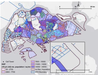
We use 2 consecutive weeks (i.e., 14 days) of mobile phone CDR data (in March and April of 2011) from one carrier in Singapore to examine the mobility patterns of anonymous individuals in the metropolitan area. The data set of the studied period contains 3.17 million anonymous mobile phone users, and a total of 722.92 million records of phone usages. There are more than 5 thousand cellular towers in Singapore, with a spacing gap of around 50-meters in the dense downtown area to a few kilometers in the suburban region. In general, the cellular tower network has a very high density covering the whole metropolitan area (see Fig.1).
3.2 Census Data and Geographic Zones
Despite the high penetration rate, data obtained from one mobile carrier for this study only count for 63% of the total population in Singapore. To get statistically meaningful measures from the CDR data for the whole population, we need to expand the sampled mobile phone users. Therefore census data with spatial information is useful. Publicly available census in Singapore includes population by differ-ent demographic groups at the planning zone level (named as Development Guide Planning zone, DGP). We assume that an individual older than 10 year-old may possess a mobile phone, and expand users in the CDR data to the population of Singapore residents in this age-category at the DGP level.
DGP is a spatial unit of planning area used by the Singapore urban planning agency—the Urban Redevelop-ment Authority (URA). There are 56 DGPs in Singapore with sizes ranging from 0.85 sq km, to 66 sq km. 35 of
these 56 DGPs have residential population residing in them, and the rest are either industrial zones or reserved land for other purposes. These DGP zones are further subdi-vided into finer-grained spatial areas, the transportation analysis zones, which are called MTZs, used for transporta-tion planning purposes by the Singapore transportatransporta-tion- transportation-planning agency—the Land and Transportation Authority (LTA). However, population data at this high spatial reso-lution (i.e., MTZ) level is not publicly available. A total of around 1100 MTZs cover the whole metropolitan area, and their sizes range from 0.015 sq km to 43 sq km.
Fig 1 exhibits the population density at the DGP level, and illustrates the spatial relationship of DGP, MTZ, and cellular towers. We expand the phone users at the tower level to match the total population at the DGP level, and estimate population at the MTZ level. We discuss the ex-pansion details in Section 4.
# # # # ## # # # # # # # # # # # ### # # # # # # # # # ### # # # ### # ### # # # # # # # # ## # # # # # # # ### # ## ### # # # # # ### # # # # # # # # # # # # # # # # # # # # # # # # # # # # # # # # # # # # ### # ### # # # # ## # # # # # ## # # # # # # # # # # # # # # # # # # # # # # # # # # # # ## # # # # #### # # # # # # # # # # # # # # # # # ##### # # # # # # # # # # # # # # # # # # # # # # # # ## # # # # # # # # # # ## # # # # # # # # # # # # # # ### # # ## # # # # #### # # # # # # # # ## # # # # # ## # # ## # # ## # # # # # # # # ### # # # # # # # # # # # ## # ### # # # # ## # # # ## # # # # # # ## # ### # # # # # ## # # # ### # # # # # # # # # # # # # # # # # # ## ## # # # # # # # # # # # # # # # # # # # # # # # ## # # # # # # # # # # # # # # # # # # # # # # # ## # ## # # # # # # # # # # # # # # # # # ## # # # # # # # # # ## # # # # # # # # # # # # # # # # # # # # # # # ## # # # # # # # # # # # # # # # # ### # # # # # # # # # # # # # # # ## ## # # # # # # # # # # # # # # # # # # # ## # # # # # # # # # # # # # # # ## # # # # # # # # # # # # # # # # ## # # # # # # # # # ## # # # # # # # ## # # ## # # # # # # # # # # # # # # # # # # # # # # # # # # # # # # # # # ## # # # # ## # ## # # ## ### # # # # # # # # # # # # # # # # # # # # # # # # # # # # # # # ## # # # # # # # # # # # # # # # # # ## # # # # # # # # # # # # # # # # # # # # # ## # ## # # # # # # # # # # # ## # # # # # ## # # # # # # # # # # ## # # # # # # # # # # # # # # # # # # # # # ## # # # # # # # # # # # # # # # # # # # # # # # # # # # # # # # # # # # # # # # # # # ## # # # # # # # # # # # # # # # # # # # # # # # # # # # # # # # # # # ## # # # # # # # # # # # # # # # # # # ## # # # # # # # # # # # # # # # ## # # # # # # # # # # # # # # # # # # # ### # # # # # # # # # ### # # # # # # # ## # # # # # # # # # # # # # # # # # # # # ## # # # # ## # # # # # # # # # # # # # # # # # # # # # # ### # # # # # # # # # # # # # # # # # # # # # # # # # # # # # # # # # # # # # # # # # # # # # # # # # # # # # # # ### # # # # # # # # # # # # # # # # ## # # # # # # # # # # # # # # # # # # # # # ## # # # # # # ## # # # # # # # # # # # # # # # # # # # # # # # # # # # # # # # # # # # # # # # # # # # # # # # # # # # # # # # ### # # # # # # # # ## # # # # # # # # # # # ## # # # # # # # # # # # # # # # # # # # # # # # # # # # # # # # # # # # # # # # # # # # ### # # # # # # # # # ## # # # # # # # # # # # # # ## # # # # # # # # # # # # # # # # # # # # # # # # # # # # # # # # # # # # # # # # # # # # # # # # # # # # # # # # # # # # ## # # # # # # # # # # # # # # # # # # # # # # # # # # # # # # # # # # # # # # # # # # # # # ## # # # # # # # # # # # # # # # # # # # # # # # # # # ## # # ## # # # # # # # # # # # # # # # # # # # # # # # ## # # # # # # # # ## # # # # # # # # # # # # # ## # # # # ## # # ## # # # # # # # # # # # # # # # # # # # ## # # # # # # # # # # # # # # ## # # # # ## # # # # # # ###### # ## # # # # # # # # # # # # # # # # # # # # # ## # # ## # # # # ### # # ## # ## # ## # # # # ## # # ## # # # # # ### # # # # ## # # # # # # # # # # # # # # # # # # # # # # # # # # # # # # # # # # ## # ## # # # # # # # ## # # # # # # # ## # # # # ## # # # # # # # # # # # # # # # # # ### # ## # # # # # # # # # # # # # ## # # # # ## # # # # # # # # # # # # # # # # # # ## # # # # # ## # # # # # # # # # # # # # # # # # # # # # # # # # # # # ## # # # # # # # # # # # # # # ## # # # # # # # # # # # # # # # # # # # # # # # ## # # # # # # # # # # # # ## # # # # # # # # # # ## # # ## # # # # # ### # # # # # # # # # # # # # # # # # # # # # # # # # # # # # # # # # # # # # # # # # ## # # # # # # # # # # # # # # ## # ## # # # # # # # # # # # # # # # # # # # # # # # # # # # # # # # # # ## # # # # # # # # # # # # # # # # # # ### ## # # # # ## # # # # # # # # # # # # # # # # # # # # # # # # # # # ## # # ## # # # # # # # # # # # # # # ## # # # # # # ### ## # # ## # ## # # # # # # ## # # # # ## # ## # # # # # # # # # # # # # ## # ## # # # ### # # # # # # # ## # # # # # ## # # ## # # # # ## # # # # # # # # # # # # # # # # # # # # # # ### # # # # # # # # # # # # # # # # # # # # # ## # # # # # #### # # # # # # # # # # # # # # ## # # # # # # ## # # # # # # # # # # # # # # # # # # # # # # # # # # # # # # # # # # # ## # # # # ## # # # ## # # # # # # # # # # ## # # # # # # # # # # # ## # # ## # # # # # # # # # ## # ## ## # # # # # # # # # # # # # ## # # # # # # # # # # # # # ## # # # # ## # # # # # # # # # # # # # # # # # ## # # # # # # # ## # # # # # # # # # ## # # # # # # # # # # # # # # # # # # ## # ## ## # # # ## # # # # # # # # # # # # # # ## # ## # ## # # # # # # # # # ## # # # # # # # ## # # # # ### # # # # ## # # # # # # # # # # # # # # # # ## # # # # # # # # # # # # # # # # # # # # # # # # # # # # # # # # # # # # # # # # # # # # # # # # # ## # # # # # # # # # # # # # ## ## # # # # # # # ## # # # # # # # # ## # # # # # # # ## # # # # ## ### # # # # # ## # # # # # # # # # # # # # # # ## # # # # # # # # ## # # ## # # ## # # # # # # # # # # # # # # # # # # # # # # ## ## # # # # # # # # # # # # # # ## # # # # # ## # # # # # # # # # ## # # # # # # # # # # # # # # # ## # # # # # # # # # # # # # # # # ### # # # # # # # # # ## # # # # # # # # # # # # # # # # # # # # # # # # # # # # # # # # # # # # # ## # # # # # # # # ## # # # # # # # # # # # # # # # # # # # # # # # # # # # # # # # # # # # # # # # # # # # # # # # # # # # # # # # # # # # # # # # # # # # # # # # # # # # # # # # # # # # # # # # # # # # # # # # # # # # # # # # # # # # # # # # # # # # # # # # # # # # # # # # # # # # # # # # # # # # # # # # # # # # # # # # # # # # # # # # # # # # # # ## # # # # # # # # # ## # # # # # # # # # # # # # # # # # # # # # # # # # # # # # # # # # # # # # # # # # # # # # # # # # # # # # # # # # # # # # # # # # # # # # # # # # # # # # # # #### # #### # # # # ###### # # # # # # # # # # # # # # # # # # # # # # # # # # # # #### # # # # # # # # # # # # # # # # # ### # # # # # # # # # # ### # # # # ## # # # # ##### # # # # #### # # # # # # # # # # # # # # ## # ## # ## # # # # # # # # # # # # # ## # # # ### # # # # # # ## ## # # # # # # # # # # ## # ## # # # # # # # # # # # # # # # # # # # # # # # # # # # # # # # # # # ## # # # # ## # # # # # # # # # # ### # ## # # # # ## # # # # # # # # # ## # # # # # # # ## # # # # # # # ### # ### # ## ### # # # # # # # ### # # # # # # # # # # # # # # # # # # # # # ## ### # # # # # # # ## # # # ## # ### # # # # # # # # # # # # # # # # ### # # # # # ## # # # # # # # ## # # # # # # # # # # # # # # # # # #### # ### # # # # # ## # # # # # # # # # # # ## # # # # # # # # ## # # # # # ## # ## # # # # # ## # # # # # # # # # # # # # # # # # # # # # # # ## # # # # # # # ### # # # # # # # # # # # # # # # # # # # # # # # #### ## # # #### # # # # # # # # # # # # # # # # # # # # # # # # # # # #### # # # ### # # #### # ## # # # # # # # # ## # # # # # # # ## # # # # # # ## # # # # # # # # # # # # # # # # # # # # # # # ## # # # ## # # #### # ## # ## # # ####### # # # # ## # # # # # # # # ## # #### # # # # # # # # # # # # # # # # # # # # # # # # ########## # # # # # # # ### # # # # # # # # # # # # # # # # # ## ## # # # # # # ####### # # # # # #### # # # # # # # # # # # ## # #### # # # # # # # # # # # # # # # # # # # # # # # # # # # # # # # # # # # # # #### # # ##### # # ### # # # # # ########## # ## # # # # # # # # # ## ########### # ## # # # # #### # # ## # # #### # # # # ## # # # # ######### # ### # # # # # ## ## # ### # # # # # ##### # # # # # # # # # # # # # # # # # # # ## # # # # # # # # # # # # # # ## # # # # ## # # # # # # # # # ###### ### # # # # # # ## # # # # # # # # # #### # # ## # # # # # # # ## #### # # # # ## # # ####### # # # # # ## # #### # # # # # ### # # # # # # # # # # #### # # # # ##### # # # ## # # # #### # # # # # # # # # # # # # # # # # # ## # # # # #### # # # ## # #### # ###### # # # # # # # # # # # # # # # # # # # ## # ######## # # # # ##### # ## # # # # #### # # # # # # # # # # # # # # # # # # # ########## # # # # # # # # # # # # ## # # # # # # # # # # # # # # # # ## # # # # # # # # ### ## # # # # # ## ## # # # # # # # # ## # # # # # # # # # ## # # # # # # # # ### # # # ## # # # # # # # # # # # # # # # # # # # ## # # # # # # # ## # # #### # # # # # # # # # ### #### # # # ## # # # # # # # # # # # # # # # # # # # # # # # # # ## # # # # # # # # # # # # # # #### # # # # # # # # # ## # ## ## # # # # # # # # # # # # # # # # ### # # # # # # # # # # ### # # # # # # # # # # # ## # # # # ## # # # # # # # # ## # # # # ## # # ## # # # # # ##### # # # # # # # # # # # # # # # # # # ## # # # # # # # ## # # # # # # # # # # # # # # # # # # # # # # # # # #### # # ### # # # # # # # # # # ## # # # # #### # # ## # # # # # # # # # # # # # ## # # # # # # # # # # # ## ## # # # # # ## ## # # # # # # # # # # # # # # # ## # # # # ## # # # # # # ## # # # # # # # # # # # # # # # # # # # # #### # # #### # # # # # # # # # # # # # # # # # # # # # # # # # # # # # # ### # # # # # # # # # # # # # ## # # ## # # # # # # # # # # # # # # # # # # # ## # # # # # # # ## # # # # # # # # # ## # # # # # ## # # # # # # ##### # # # # # # ### # # # # # # # # # # # # # # # # # # # # # # ## ######## # # # ## # # # # # # ## # # # # # # # # # # # # # # # ## # # # # # # # # ## # # # # # ## # # # # # # # # # # # # # # # # # # # # # # # # # # # # # # # # # # # # # # # # # # # # # # ## # # ## # # # # # # # # # ### # ## # # # # # # # # # # # # # # # # # # # # # ## # # # # # # # # # # # # # # # # # # # # ## # # # # # # # # # # # # # # ## # # # # # # # # # # # # # # # # # # # # # # # # # # # # # # # # # # # # # # # ## # # # # # # # # # ## # # # # # # # # # # ## # # # # # # ## # # # # ### # # # # # # # # # # ## # # # # # # # # # # # # # # # # # # # # # # # # # # # # # # # # # # ## # # # # # # # # # # # # # # # # # # # # ## # # # # # ## # # # # # # # # # # # # ## # # # # # # # # # # # # # # # # # # # # ## # # # # # # # # ## # # # # # # # ## # # # # # # # # # # # # # # # # # # # # ### # # # # # # # # # # # # # # # # # # # # # # # # # # # # # # # # # # # # # # # # # # # # # # ## # # # # # # # # # # # # # # # # # # # # # # # # # # # # # # # # # # # # # # # # # # # # # # # # # # # # # # # # # # # # # ## # # # # # # # # # # # # # # # # # # # # ## # ## # # # # # ## # # # # # # # # ## # # # # # # # # # # # # # # # # # # # # # # # # ## # # # # # # # # # # # # # # # # # # # # # # # # # # # # # # # # # # # # # # # # # # # # # # # # # # # # # # ## # # # # # # # # # # # # # # # # # # # # # # # # # # # # # # # # # # # # # # # # # # # # # # # # # # # # # # # # # # # # # # # # # # # # # # # # # # # # # # # # # # # # # # # # # # # # # # # # # # ## # # # # # # # # # # # # # # # # # # # # # # # # # # # # # # # # # # # # # # # # # # # # # # # # # # # # # # # # # # # ## # # # # # # # # # # # # # # # # # # # #
Esri, HERE, DeLorme, MapmyIndia, © OpenStreetMap contributors, and the GIS user community
# Cell Tower
DGP
(>9 yrs old) res. population / sq km 39 - 2700 2800 - 7700 7800 - 10000 11000 - 13000 14000 - 34000 no Res. Population MTZ Boundary
±
0 1 2km 0 10 20kmFig. 1. Singapore Development Guide Planning (DGP) zones, trans-portation analysis zones (MTZ), and cellular towers.
3.3 Survey Data
We use the Singapore 2008 Household Interview Travel Survey (HITS) data collected by the Singapore LTA to validate results estimated from the CDR data. Compared with CDRs, travel survey data are often in a small sample-sizes and come with expansion factors for the purpose of expanding survey samples to total population. Survey expansion factors are derived from sampling design based on individual demographics (e.g., age, gender, etc.). Survey data includes detailed information on household and indi-vidual social demographics and travel records self-reported by survey respondents. The Singapore 2008 HITS includes 34,000 individuals and their 1-day travel information (e.g., trip arrival and departure time, trip purpose, location of trip origins and destinations, etc.). In this study, we use the travel time and location information and expansion factors to expand survey samples to the population, and compare results with estimates from the CDR data.
4
METHODS
To understand human mobility patterns at the metropolitan level for urban and transportation planning purposes, in
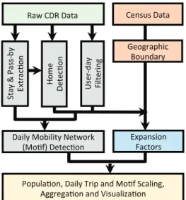
this study, we synthesize methods in previous research [24], [29], [35], and develop a pipeline of (1) parsing the CDR data to extract stay locations of phone users; (2) detecting phone users’ home location; (3) filtering users and select sta-tistically representative samples from the parsed CDR data; (4) identifying the daily mobility networks of the phone users; (5) deriving expansion factors for the filtered phone observations by combining processed phone data and the census data; expanding cellphone-users, trips, and daily motifs; and aggregating them from tower to transportation analysis zones. (see Fig.2)
Fig. 2. Workflow of population estimation and mobility pattern extraction from CDR data.
4.1 Parsing Trajectory to Extract Stays
Parsing the mobile phone CDR data to extract anchor points (i.e., stay locations) of individual daily travel and to differentiate stops from pass-by points is the first stage before identifying individual mobility networks. Zheng [28] presents a comprehensive overview on trajectory data min-ing. Inspired by the algorithm introduced by Hariharan and Toyama [40] which was tested previously using triangulated mobile phone data [24], [29], we modified the algorithm for the tower-based CDR trajectories in this study. Other algo-rithms on stay detection can also be found in the literature [41], [42]. While detecting stays, we aim to achieve three goals: (1) eliminating two types of noises in the raw CDR data—outliers and signal jumps between towers of users’ geospatial location records—to identify their true location, (2) clustering points that are spatially close (within the threshold of ∆d) and temporally adjacent (in the sequence) into a single location, with a collapsed time duration in-ferred from this clustering as the stay, and (3) agglomerating points that are spatially close but not necessarily adjacent in temporal dimension into one unique location.
• Considering a user i’s location recorded in the CDR in sequence as Di = (di(1), di(2), ..., di(ni)), by
selecting a roaming distance ∆d1 (e.g., 300 meters)
as the threshold, we heuristically cluster spatially close locations within ∆d1 for each point into their
medoid (the point in a set that minimizes the max-imum distance to every other point in the set) and form a new sequence Di0 = (d0i(1), d0i(2), ..., d0i(n0i),
where di(k) = (tower(k), t(k)) for k = 1, ..., ni;
tower(k) and t(k) are the tower id, and time stamp of the user i’s k-th observation in the raw CDR data. d0i(g) = (cellid(g), t(g), dur(g)) includes the tower id, starting time of the first observed tower in the cluster, and the duration that the user stayed in the cluster.
• Then further cluster the points in the trajectory sequence set Di0 based on the distance threshold
of ∆d2 (e.g., 300 meters), and keep the points
whose duration are greater than the time thresh-old ∆t (e.g., 10 minutes) as the final stay points Si = (si(1), si(2), ..., si(mi)), where si(m) =
(cellid(m), t(m), dur(m)). By doing so, we eliminate outliers in the clustering process. Fig3 illustrates the input and output of the process.
Fig. 3. Stay point detection.
4.2 Detecting Home
It is important to label the mobile phone users’ home loca-tion (tower) for several reasons. First, when we later expand the users to population, we need to combine CDR data with census data, which only record population by residential location. Second, in order to form mobility networks we make an assumption that for each day, an individual always departures from home and returns home by the end of a day. Although in the real world there are exceptions, this assumption simplifies the way we extract mobility networks from CDR data and allows us to estimate trips in a justifiable way. Since CDR data passively records phone users’ spatiotemporal information, it does not always give complete information of individuals’ whereabouts. Third, for planning purpose, it is important to understand indi-viduals’ mobility patterns from their home, as the built environment and land use of individual residence influence their travel and activities [43], [44]. Being able to identify human mobility patterns associated with urban space will enable planners to target future urban development and improvement.
A phone user’s home tower is identified as the most frequently communicated tower during nights of weekdays, and weekends over the study period (i.e., 14 days in this study). The definition of ’night’ is a parameter that can be adjusted in different urban contexts. We define a night from 7 pm to 7 am in this study based on the local context in Singapore.
After processing the CDR data, we obtained 2.88 mil-lion users whose home towers can be observed in the 2-week data. It counts for 91% of all phone users contained in the data for the study period, and around 56% of the total population. By properly expanding these users, we can disaggregate population from aggregated planning area level (DGP), to the neighborhood transportation analysis zone (MTZ) level with high spatial resolution. We discuss the population expansion method and results in Section 4.5.
4.3 Filtering Phone User-Day Samples
Compared with traditional survey data, the advantage of the CDR data is the longer observation period and larger sample size, and its disadvantage is the sparseness of the data. CDRs may not always reveal individual travel as travel dairies or GPS tracking applications do. Therefore it is im-portant to sample user-days when the mobile device is used frequently enough. Previous research [35] has found that if a cellphone user’s phone communication activities exceed a certain threshold, the CDR data can be treated equivalently as survey data, and generate statistically consistent and comparable results in terms of individual mobility patterns. In this study, we adopt similar rules for the sample filtering, as follows.
• Only keep a user-day observation, if in a day (24 hours) the user has phone records in at least 8 distinct time-slots of the 48 half-hour time-slots.
• Separate observations on weekdays from those on weekends, as mobility patterns can be different. Here we only focus on records on weekdays.
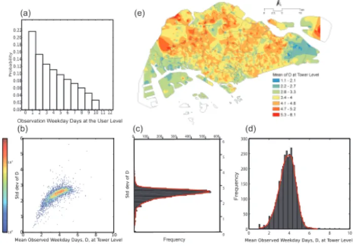
After the filtering, we keep 6.28 million user-days for 1.55 million users in the 10 weekday days of the two weeks. The total number of users after filtering is 49% of all users in the raw data. We plot the frequency distribution of user-days per user after the filtering in Fig4 (a). We can see that, for these filtered 1.55 million users, 22% of them only have 1-day observation, 11% 4 days, 7% 7 days, and 3% 10 days. On average, each user has 4 weekday observations. We then aggregate the user information to the tower level. Fig4 (b) shows the density distribution of the standard deviation (shown separately in Fig4(c)) and the mean (shown separately in Fig4(d)) of the users’ number of observation days at the tower level based on users’ home tower. We plot the spatial distribution of the mean of the users’ number of observation days at the tower level in Fig 4 (e). We can see that in downtown, airport, and the west-end of the coastal area, the number of user-day per user is relatively low. Presumably, tourists and foreigners live in these areas. While in residential areas in the suburbs, such as Ang Mo Kio, Bukit Batok, Jurong West, Punggol, Sengkang, Tampines, Yishun, and Woodlands, the average numbers of user-days are relatively higher than average.
4.4 Identifying Activity-Based Mobility Patterns
4.4.1 Daily Mobility Motifs
Human daily mobility can be highly structural—organized by a few activities essential to life. It is important to identify individual mobility networks (i.e., daily motifs).
0 2 4 6 8 10 0 50 100 150 200 250 300 Frequency 0 1 2 3 4 5 6 0 100 200 300 400 500 600 Frequency Frequency
Observation Weekday Days at the User Level
(a)
(b) (c) (d)
(e)
Fig. 4. User-day statistics after sample filtering: (a) frequency distribution of total number of days for each user; (b) density distribution of the standard deviation (shown in c) and mean (shown in d) of the users’ number of observation days at the tower level; (e) spatial distribution of the mean of the users’ number of observation days at the tower level.
The most contemporary travel demand models developed and employed by regional transportation agencies in the developed countries are activity-based [33]. Fig 5 (1a-1f) shows some examples of individual activity pattern (daily tours) commonly observed in travel surveys. Represented in the transportation modeling language, they are: (1a) 1 home-based work tour, (1b) 1 home-based work tour with a third destination, and work as the primary destination, (1c) 1 home-based work tour with 1 home-based sub-tour, (1d) 2 home-based work tours with a third destination, (1e) 1 home-based work tour with 1 work-based sub-tour, and (1f) 1 home-based work tour with 1 escort tour (to drop off and pick up somebody). These activity patterns can go into numerous combinations. However, if we use a more abstract diagram to represent these activity-chains, they can be reduced into daily motifs captured by the massive and passive mobile phone data. Fig 5 (2a-2f) represents (1a-1f) in a highly abstract format, called daily motifs. They have been proposed and tested as measures of human mobility in previous studies for Paris, Chicago and Boston [24], [35], and have been found comparable to travel surveys in aggregated statistics. home drop off work pick up home work shop home work shop home work lunch shop home work dinner home work (1a) (1b) (1c) (1d) (1e) (1f) (2a) (2b) (2c) (2d) (2e) (2f)
Fig. 5. Examples of daily mobility networks (1a-1f) in daily travel surveys, and (2a-2f) in abstract.
Here, we present the algorithm to identify the daily mo-tifs for the filtered phone users whose mobile phone records in a sampled day are frequent enough (explained in Section 4.3) for representing their daily activity pattern. Formally
speaking, a motif is an equivalence class of directed graphs. A directed graph is an ordered pair D = (V, A) where V is the set of nodes (or vertices), and A is a set of ordered pairs of nodes (i.e., directed edges). Without loss of generality, when V is a set of n elements, we take V to be the set Vn, {1, 2, . . . , n}. Let Dnbe the set of directed graphs with
n nodes, i.e., Dn , {Dn| Dn= (Vn, A), A ⊆ Vn× Vn}. The
motifs [Dn] ignore the labeling of the nodes.
With the extracted stay locations, including observed and potential stay locations (described in Section 4.1) and users’ identified home location (discussed in Section 4.2), we will be able to identify the mobility networks as illustrated in Fig 5 (2a-2f). We find that not all users necessarily have the first stay-point (or potential stay-point) starting from their home tower, or the last stay point (or potential stay-point) ending at their home tower every day in the filtered trajectory, due to the passive nature of the CDR data. In order to form a complete tour for each user, we make the assumption that, if a user travels in a day, s/he starts the first trip from, and ends the last trip at home.
• From the extracted stay points and filtered day(s), we
obtain a sequence of destinations on the sampled day k, for a given anonymous user i, denoted by Sik =
(sik(1), sik(2), ..., sik(mik)).
• User i’s home hiwas detected in previous step. • Always check if for day k, user i’s first and last
activity locations are hi. If not, we add home hi to
the stay point sequence, which forms a new sequence Sik0 = (s0ik(1), s0ik(2), ..., s0ik(m0ik)).
• Count total number of trips (which are journeys from
origins to destinations), lik, for user i on day k. • Count total number of distinct nodes, nik, from
tra-jectory Sik0 .
• Form a network (directed graph) Dikwith niknodes:
using an nik × nik matrix Mik, we represent the
mobility network for user i on day k. If there is at least one trip from node o to node d, Mik(o, d) = 1;
otherwise, Mik(o, d) = 0.
• Obtain motif [Dik], i.e., the equivalence class of Dik.
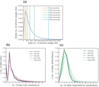
4.4.2 Mobile Phone Usage Patterns and Mobility Patterns After filtering the user-day samples, it is important to verify that users with more phone usage events do not have systematic differences in travel behavior. To this end, we examine the relationship between the filtered users’ cell phone usage patterns and their daily travel patterns. Fig 6 (a) presents the frequency distribution of total number of phone usage observations for all the 1.55 million filtered users in the 10 weekday days. The 5th, 20th, 40th, 60th, 80th, and 95th percentiles of the total phone usages during this period for all the filtered users are 140, 262, 420, 650, 1108, and 2558, respectively. Based on this information, we group the filtered users into 5 groups, with total phone usage observations of [100, 200), [200, 400), [400, 600), [600, 1000), and [1000, 2500). We examine the filtered users’ daily travel patterns, including daily number of trips, and daily number of unique destinations for each of the groups. Fig 6 (b) shows that for these 5 groups of filtered users, the frequency distributions of their daily number of trips are quite similar across the groups. Similarly, Fig 6 (c) shows
that the frequency distributions of daily number of unique locations visited by the filtered users of various groups also follow similar patterns.
(a)
(b) (c)
Fig. 6. Frequency distribution of (a) total no. of phone usages for filtered users, (b) weekday daily no. of trips for filtered user-day samples by user group, and (c) weekday daily no. of unique locations for filtered user-day samples by user group.
It indicates that phone users with different phone usage patterns do not have systematic differences in travel behav-ior. This verification is critical to the validity of using active mobile phone user-day samples to further examine human daily mobility patterns, and use these samples to expand to the population.
4.5 Expanding Mobile Phone Sample to Population
To derive estimates of trips and daily mobility patterns (motifs), and robust spatial patterns for the population in the metropolitan area, and informative for city planning and transportation planning, we need to expand the mobile phone samples (including users and user-days) properly. In this section, we describe the process in generating the expansion factors for the CDR data.
4.5.1 Expansion Factors
Two types of expansion factors are generated, including (1) user expansion factors, and (2) user-day expansion factors. Fig 7 presents the entity relationship diagram useful in gen-erating these expansion factors. After detecting the mobile phone users’ home towers, we store the users’ information in a database table “user”, with their anonymized id num-ber that is unique to each user. Home towers of 2.88 million users were detected. We store the mobility patterns of the filtered users who had frequent phone communication ac-tivities (in at least 8 half-hour time slots in a day) in the table “user day motif ”, in which each row represents a unique user-day observation, with user id, motif id, and number of trip information. 6.28 million user-day records are included in this table for 1.55 million unique users whose home tower information can be found in the “user” table. The rest of the 1.33 million users, who are in the “user” table but not in the “user day motif ” table, are those whose
phone communication activities are not enough to meet the filtering threshold.
As exhibited in Fig 7, the “user” table is linked to the “cell tower” table through the “cell tower id” of the users’ “home tower id”. By the spatial operation of joining cell towers to the MTZ zones that they fall into, each cell tower is associated with an MTZ. For those towers, which are not contained in any MTZs, the nearest MTZ within a 200-meter distance is used to allow for the measurement error in spatial representation of zone and tower location. The “cell tower’ table is linked to the “mtz taz” table (through “mtz id”), which is then linked to the “planning area” table (through “dgp id”), including 56 DGP zones of which 35 contain residential population.
Fig. 7. Entity relation diagram of the processed mobile phone user, user-day mobility data from their CDRs, and geographic spatial units: towers, transportation analysis zones (MTZs), planning area (DGPs) with census population.
Two sets of expansion factors are considered. One in-cludes the user expansion factors calculated for the 2.88 million users with identifiable home location; the other includes user expansion factors for the 1.55 million users and the user-day expansion factors for the 6.28 million user-day observations (from the 1.55 million users). For the former case, the user expansion factor for every user with home tower in the same planning area is the same. For the latter case, as each user may have observations for more than one day, we normalize the expansion factor by the total number of observation-days for this user. We define the user expansion factor βi for user i, and the user-day expansion
factor θikfor user i on day k as follows. • βi= Pg/P
Qg
1 Uhg , for user i with a home tower hg.
Where Pg is the population (above 10 years old) in
DGP zone g reported in the census; Uhg is the total
number of users whose home tower is at hg in DGP
zone g, and Qgis the total number of towers in zone
g;
• θik = βi/Ki, where Ki is the total number of days
when the user i’s motifs are identified.
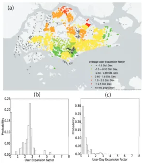
In Fig 8 (a) we present the spatial distribution of the user expansion factors at the tower level across Singapore, color-coded by different brackets of the expansion factors based on the ranging of the standard deviation measure. We can see that the user expansion factors are higher in the north part of Singapore, meaning that phone user to
the population ratio in this region is lower than the city average. However, when looking at Fig 4 we see that for an average phone user in this north region, she or he tends to have relatively more days of observations. In the central region, the user-expansion factors are lower, meaning that the phone user to population ratio in this region is higher than the city average. Fig 8 (b) and (c) present the frequency distribution of user expansion factors (for the 1.55 million phone users) and user-day expansion factors (for the 6.28 million user-day observations), respectively.
Fig. 8. (a) Spatial distribution of user-expansion factors at the tower level, and frequency distribution of (b) user-expansion factors,and (c) user-day expansion factors.
4.5.2 Population Estimation in High Resolution
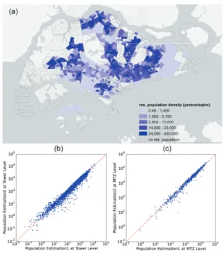
With the estimated expansion factor for each phone user in the study, we can then estimate population with high spatial resolution that are not available in the census statistics but are useful for the transportation and urban planning. Fig 9 (a) presents the estimated residential population density (for people older than 10 years old) in Singapore at the MTZ level (with more than 1100 zones) by using the CDR data. To compare the population estimates from users who only have home location detected (denoted as Estimation 1), with the estimates from the filtered user whose mobility patterns can be identified (denoted as Estimation 2), we plot the two population estimates at the tower level, and at the MTZ level in Fig 9 (b) and (c) respectively. We can see that with proper treatment of expansion, by only using the frequent user-observations (although a smaller sample size), it can provide comparable estimates to those by using all user samples whose home location can be detected without filtering (based on their phone usage frequency). The benefit of using the filtered phone users (based on their phone com-munication frequency) is that we can mine richer mobility patterns from their records, and treat these observations as travel survey in a much larger scale, to inform sound city planning and make wiser decisions on public policies related to urban and transportation development.
Fig. 9. (a) Residential population density estimates at the MTZ level; (b) comparison of population estimation from the sample with all users with detected home (a.k.a. Estimation 1), and filtered users with complete motility networks (a.k.a., Estimation 2) at the tower level, and (c) at the MTZ level.
4.5.3 Aggregating Daily Trips and Mobility Patterns After applying the expansion factors to the user-day ob-servations, we aggregate the daily trips and mobility pat-terns for Singapore residents (above 10 years old) at the metropolitan level, and infer human mobility patterns for Singapore. Fig 10 presents the inferred frequency distribu-tion of (a) daily mobility patterns, (b) the number of daily trips, and (c) the number of unique daily destinations that the mobile phone users visited during weekday. Fig 10 (a) also compares the results obtained from CDR data with the estimates from the HITS travel survey data. From the mobile phone data, we find that on an average weekday, 13.5% Singapore residents stayed at home, 33% visited 2 unique places, 30% 3 places, 14% 4 places, 5.5% 5 places, 2.1% 6 places, and less than 2% visited more than 6 places. These patterns cover around 90% of survey respondents’ travel.
When comparing the estimates of daily motifs with survey data, in Fig 10 (a) we find that the motif with 2-nodes reported in the survey is dominant (55%), and much higher than those observed from the CDR data. We find the following reasons for explanation. (1) The HITS survey only asks for motorized travel, and excludes non-motorized travel. (2) People tend to under-report their secondary des-tinations to the primary desdes-tinations in the survey than the mobile phone could detect. If we refer to travel survey data in other metropolitan areas such as Chicago, Boston, and Paris, we found that the 2-node travel patterns are always less than 40% [24][35].
A separate study [45] that uses smartphone-based sur-vey to track and record individual users’ travels and activ-ities in Singapore conducted by the Future Mobility Survey (FMS) project confirms similar observation. Even though
13.5% 33.0% 15.5% 9.4% 4.4% 4.3% 4.2% 1.3% 0.8% 1% 1% 23.4% 55.2% 5.8%3.7% 0.0% 10.0% 20.0% 30.0% 40.0% 50.0% 60.0% 1000 2002 3003 3004 3005 4005 4004 4006 4008 5005 5006 phone survey 0 10 20 0 0.1 0.2 0.3 0.4
Weekday Daily Trips, t
p (t) 0 5 10 0 0.1 0.2 0.3 0.4
Weekday Daily Destinations, d
p (d ) (a) (b) (c) 1 2 3 4 5 6 7 8 9 10 11 Motif ID p (I D )
Fig. 10. (a) Daily motifs derived from CDR and survey data, and (b) frequency distribution of daily trips, and (c) activity destinations from CDR data.
the FMS project only has 387 individuals who answered both the paper-based survey and validated their travel in the smartphone app based tracking survey, it is observed that people significantly under report their travel in the paper-based survey. 76.3% people in the paper-based survey reported 2 trips, while only 20% were detected and verified that they had 2 trips in the smartphone based survey. There-fore, the mobility patterns inferred from the phone CDR data here can be more reasonable than the travel survey data. This difference will have a significant impact on policy implications for urban and transportation planning.
5
SPATIAL
PATTERNS OF
ACTIVITY-
BASEDHU-MAN
MOBILITY
Understanding the spatial patterns of human mobility ag-gregated at their home location is especially important to help planners understand how their neighborhood and the built environment may influence their travel. A vast body of literature in planning [46] has tried to test this theory empirically using traditional travel survey data. With the method presented in this study, we can derive new evi-dences on people’s travel behavior in a large scale, and facilitate planners and policy makers to identify areas with great potential for improvement, such as provision of trans-portation alternatives to reduce motorized travel, improve-ment of community facilities to targeted population. In this section, we present analytical indicators to measure the spatial distribution of mobility patterns from the perspective of individuals’ home location.
5.1 The 2-node Home-based Tour
Fig 11-b presents the population density of residents with only 2-node motifs. These residents had one additional place besides ’home’ that is important in their daily life. It could be workplace for workers, school for students, or a
social/recreational place for the non-workers/non-students. Since they are the majority of the population (around 33%, shown in Fig 10-a), the spatial distribution of the group with 2-node motifs is very similar to the spatial distribution of total population (shown in Fig 9-a). We use the concept of Location Quotient, to compare an area’s distribution of resi-dents by mobility type to the distribution of a reference area (i.e. the Singapore metropolitan area). To be more specific, for example, to measure how residents with daily motif m are concentrated in a particular neighborhood (at the MTZ level) compared to the population in the metropolitan area, we use the Location Quotient (LQm), detailed as follows.
• LQm= (em/e)/(Em/E), where emis the residential
population with daily motif type m (Fig 9-a) in a zone (e.g., MTZ); e is the total residential population in zone; Emis residential population with daily motif
type m in the metropolitan area (e.g., Singapore); E is the total residential population in the metropolitan area.
From Fig 11 (a) and (c), we can see that several sub-urban neighborhoods have a unique identity with a greater than metropolitan average share of residents whose daily mobility networks are of 2 nodes. These areas include zones in the West region, such as Jurong East, Jurong West, Clementi, Bukit Batok, Choa Chu Kang; zones in the North-West region, including Woodlands, Sembawang, and Yishun; zones in the North-East region such as An Mo Kio, Sengkang, and Punggol; and zones in Bedok of the East region (see Fig 11-a for zone name references). People who only visit 1 other place besides their home (for work/school as the majority) are overly concentrated in these zones, which are new towns and far away from the city cen-ter. It would be potentially important to provide public transportation services with high capacity and frequency during the peak-hour to relieve congestion for residents in these neighborhoods. Meantime it is also important to plan more localized economic and community services in these neighborhoods to help reduce long distance travel for the needs of additional activities.
5.2 The 1-node, 3-node and 4-node Motifs
As the 2-node home-based tour pattern (see Fig 10) is the majority of mobility patterns in the metropolitan area, we also use it as a reference, and compare other types of mobility patterns to the spatial distribution of the 2-node pattern, and we call it the Relative Location Quo-tient, RLQd = LQd/LQ2, for motif type d. Fig 11 (d-f)
highlights MTZs that have high concentration of stay-at-home residents, and residents with 3-node, and 4-node in their daily activity motifs, respectively. Fig 11 (e) and (f) collapse the spatial distribution of the different motifs with 3-node, and with 4-node into one map. Fig 11 only shows areas with population (for the corresponding type of motif) greater than 500 persons, and population density (for the corresponding type of motif) higher than 1500 person per sq km. We also only show areas that their Location Quotient, and Relative Location Quotient (to 2-node) exceed 1.05 (to allow for 5% error), to illustrate the highly concentrated areas with the corresponding types of daily motifs for
residents living in the zones. Fig 11 (a) overlays the highly concentrated zones of residents with 2-node, 3-node, and 4-node in different colors, and illustrates the overall patterns of mobility of Singapore residents. We can see that weekday stay-at-home residents are highly concentrated in zones in the Central region and along the east coast, and in zones of the North-west region, and some areas in the West region. In the Central region, it contains more mature neighborhoods where senior residents have higher probability to reside.
Fig12 zooms into the neighborhoods containing highly concentrated residents with 3- and 4-node motifs demon-strated in Fig11(a). We can see that these area include suburbs that are connected by light rail (grey lines in the figure) to the major transit lines, such as Bukit Panjang, and Bukit Bakok in the West region (Fig12-a), and Sengkang in the North-East region (Fig12-b), where accessibility are relatively low. It also includes areas that are currently not served by the MRT, such as Lentor, Mayflower, Bright Hill and Upper Thomason, in Ang Mo Kio and Bishan (Fig12-c), and neighborhoods in the north part of Bedok and Tempines (Fig12-d). Neighborhoods that have higher concentration of residents of 3- and 4-node motifs usually have more trips. By providing more convenient public transportation serveries, improved level of services (e.g. for the light rail), and alternative transportation modes can help reduce total travel. It’s worth noting that in some areas, the Singapore LTA has provided plans to improve transit network (and some of them are under construction as depicted in grey dashed line in Fig12-c and d).
6
CONCLUSIONS
Sustainable urban and transportation planning depends greatly on understanding human mobility patterns in the metropolitan area. In this paper, we present an integrated pipeline that can parse, filter, and expand the raw passive and massive mobile phone CDR data to extract human mobility patterns for millions of anonymous residents in a metropolitan area, and translate the knowledge gained into planning-interpretable languages. Traditional travel survey data, although rich in detail, can be misleading. It may gen-erate inaccurate mobility patterns due to incomplete self-reports, lead to biased travel demand models—especially for non-work trip purposes—and result in inefficient re-source allocation and ill-informed plans. Big Data, if prop-erly treated, can provide further insights beyond travel sur-veys, supporting multiple-day observations, revealing more robust mobility patterns, and covering wider geographic ar-eas. The method presented in this paper differs from existing studies that utilize CDR data to examine human travels in a trip-based approach [26], [38]. Rather, it is activity-based and focuses on patterns of tours and trip-chaining behavior in daily mobility networks.
As the literature suggests, in light of changing urban economic structure, diverse workforce participation, and flexible working schedule, trip-chaining behavior has be-come more complex. Policies for peak-hour congestion mit-igation or VMT reduction that ignore the increasing need to chain non-work trips into commuting trips or focus only on travel speed improvements or travel cost incentives could be less effective than expected [47]. Moreover, the method
pre-East West North-West Central East North-East Central West Jurong Industrial Central Area 1 4 13 8 2 22 9 24 6 11 23 25 21 3 5 26 18 12 14 19
Esri, HERE, DeLorme, MapmyIndia, © OpenStreetMap contributors, and the GIS user community
East West North-West Central East North-East Central West Jurong Industrial Central Area
Esri, HERE, DeLorme, MapmyIndia, © OpenStreetMap contributors, and the GIS user community
Esri, HERE, DeLorme, MapmyIndia, © OpenStreetMap contributors, and the GIS user community
Esri, HERE, DeLorme, MapmyIndia, © OpenStreetMap contributors, and the GIS user community Esri, HERE, DeLorme, MapmyIndia, © OpenStreetMap contributors, and the GIS user community Esri, HERE, DeLorme, MapmyIndia, © OpenStreetMap contributors, and the GIS user community
population density (2 node) per/sq km 1.2 - 1500 1600 - 5000 5100 - 120000
2 Node (per density>1500)
LQ>1.05
1 Node (per density>1500) LQ>1.05 & RLQ>1.05
3 Node (per density>1500)
LQ>1.05 & RLQ>1.05 4 Node (per density>1500)LQ>1.05 & RLQ>1.05
DGP URA Names 1, Ang Mo Kio 2, Bedok 3, Bishan 4, Bukit Batok 5, Bukit Merah 6, Bukit Panjang 7, Bukit Timah 8, Choa Chu Kang
9, Clementi 10, Geylang 11, Hougang 12, Jurong East 13, Jurong West 14, Kallang 15, Marine Parade 16, Novena 17, Outram 18, Pasir Ris 19, Punggol 20, Seletar 21, Sembawang 22, Sengkang 23, Tampines 24, Toa Payoh 25, Woodlands 26, Yishun 3 Node 4 Node 2 Node
(a)
(b)
(d)
(e)
(f)
(c)
Fig. 11. Highly concentrated areas with residents of (c) 2-node, (d) 1-node (stay-at-home), (e) 3-node, (f) 4-node, and (a) overlay of 2-node, 3-node, and 4-node mobility networks; and (b) population density of residents with 2-node motifs. (Note: aggregation based on phone users’ home location).
1
3
Esri, HERE, DeLorme, MapmyIndia, © OpenStreetMap contributors, and the GIS user community
22 11
20 19
Esri, HERE, DeLorme, MapmyIndia, © OpenStreetMap contributors, and the GIS user community
2 23
18
Esri, HERE, DeLorme, MapmyIndia, © OpenStreetMap contributors, and the GIS user community
6 8
4
Esri, HERE, DeLorme, MapmyIndia, © OpenStreetMap contributors, and the GIS user community
3 Node 4 Node 0 0.5 1km 0 0.5 1km 0 1 2km 0 0.5 1km (a) (b) (c) (d)
Fig. 12. Neighborhoods with high concentration of residents with 3-node and 4-node daily motifs (with zone reference names in Fig11-a).
sented here can be further extended to examine more details at clusters with 1- or 2- node versus 3- or 4-node motifs— including understanding the demographics, housing types
of the clusters, calling for a next-level investigation that sorts motifs by tour length. With the types of tools presented here, planners can derive new evidences on people’s travel behavior on a large scale using ubiquitous data from com-munication technologies. By understanding the different patterns of human mobility for different neighborhoods at the metropolitan scale, planners can design policies that target neighborhoods with great potential for improvement. The large-scale behavior evidence can be used to arrange shopping clusters along certain stops for transit-oriented development, add transportation alternatives and improve level of service along certain corridors. Other applications include improving community facilities for targeted pop-ulation, or integrating land-use transportation planning to reduce total travel and its negative social and environmental externalities.
ACKNOWLEDGMENTS
This research was in part funded by the Singapore Na-tional Research Foundation (NRF) through the Singapore-MIT Alliance for Research and Technology (SMART) Center for Future Urban Mobility (FM) and by the Center for Complex Engineering Systems (CCES) at KACST. We thank data providers for research collaboration through SMART.
REFERENCES
[1] K. Lynch,The Image of the City. Cambridge, MA: The MIT
Press, 1964.
[2] T. Carlstein, D. Parkes, and N. Thrift, “Human activity and time geography,” 1978.
[3] T. Hgerstrand, “What about people in regional science?,”Pap. Reg.
Sci., vol. 24, no. 1, pp. 7–24, 1970.
[4] S. Jiang, J. Ferreira, and M. C. Gonzlez, “Clustering daily patterns
of human activities in the city,”Data Min. Knowl. Discov., vol.
25, no. 3, pp. 478–510, Apr. 2012.
[5] M. Batty, “Cities as Complex Systems: Scaling, Interactions,
Net-works, Dynamics and Urban Morphologies,” in Encyclopedia of
Complexity and Systems Science, vol. 1, R. Meyers, Ed. Berlin, DE: Springer, 2009, pp. 1041–1071.
[6] D. Zhang, M. Philipose, and Q. Yang, “Introduction to the special
issue on intelligent systems for activity recognition,”ACM Trans.
Intell. Syst. Technol., vol. 2, no. 1, pp. 1–4, Jan. 2011.
[7] D. Zhang, B. Guo, and Z. Yu, “The Emergence of Social and
Community Intelligence,”Computer, vol. 44, no. 7. pp. 21–28,
2011.
[8] “Data for Development (D4D) Challenge.” [Online]. Available: http://d4d.orange.com/en/Accueil.
[9] J. Wakefield, “Mobile phone data redraws bus routes in Africa,” BBC, 01-May-2013.
[10] E. Cho, S. A. Myers, and J. Leskovec, “Friendship and mobility:
user movement in location-based social networks,” inProceedings
of the 17th ACM SIGKDD international conference on Knowl-edge discovery and data mining, 2011, pp. 1082–1090.
[11] S. Elwood, M. F. Goodchild, and D. Z. Sui, “Researching Volun-teered Geographic Information: Spatial Data, Geographic Research,
and New Social Practice,”Ann. Assoc. Am. Geogr., vol. 102, no.
3, pp. 571–590, 2012.
[12] Y. Zheng, L. Capra, O. Wolfson, and H. Yang, “Urban Computing,” ACM Trans. Intell. Syst. Technol., vol. 5, no. 3, pp. 1–55, Sep. 2014.
[13] M. Batty,The New Science of Cities. MIT Press, 2013.
[14] N. Eagle, A. Pentland, and D. Lazer, “Inferring friendship network
structure by using mobile phone data,” Proc. Natl. Acad. Sci.,
2009.
[15] F. Calabrese, M. Colonna, P. Lovisolo, D. Parata, and C. Ratti, “Real-Time Urban Monitoring Using Cell Phones: A Case Study
in Rome,”IEEE Trans. Intell. Transp. Syst., vol. 12, no. 1, pp.
141–151, 2011.
[16] N. Caceres, J. P. Wideberg, and F. G. Benitez, “Deriving origin
destination data from a mobile phone network,”Intell. Transp.
Syst. IET, vol. 1, no. 1, pp. 15–26, 2007.
[17] C. Ratti, D. Frenchman, R. M. Pulselli, and S. Williams, “Mobile landscapes: Using location data from cell phones for urban
analy-sis,”Environ. Plan. B Plan. Des., vol. 33, no. 5, pp. 727–748,
2006.
[18] M. C. Gonzlez, C. A. Hidalgo, and A.-L. Barabsi, “Understanding
individual human mobility patterns,”Nature, vol. 453, no. 7196,
pp. 779–782, Jun. 2008.
[19] F. Girardin, F. Calabrese, F. D. Fiore, C. Ratti, and J. Blat, “Digital Footprinting: Uncovering Tourists with User-Generated Content,” IEEE Pervasive Computing, vol. 7, no. 4. pp. 36–43, 2008. [20] V. D. Blondel, A. Decuyper, and G. Krings, “A survey of results
on mobile phone datasets analysis,”EPJ Data Sci., vol. 4, no. 1,
2015.
[21] F. Calabrese, L. Ferrari, and V. D. Blondel, “Urban Sensing Using
Mobile Phone Network Data: A Survey of Research,”ACM
Com-put. Surv., vol. 47, no. 2, pp. 25:1–25:20, Nov. 2014.
[22] C. Song, T. Koren, P. Wang, and A.-L. Barabasi, “Modelling the
scaling properties of human mobility,”Nat Phys, vol. 6, no. 10,
pp. 818–823, 2010.
[23] C. Song, Z. Qu, N. Blumm, and A.-L. Barabsi, “Limits of
pre-dictability in human mobility.,”Science, vol. 327, no. 5968, pp.
1018–1021, 2010.
[24] S. Jiang, G. a Fiore, Y. Yang, J. Ferreira, E. Frazzoli, and M. C. Gonzlez, “A review of urban computing for mobile phone traces,” inProceedings of the 2nd ACM SIGKDD International Workshop on Urban Computing - UrbComp ’13, 2013
[25] V. W. Zheng, Y. Zheng, X. Xie, and Q. Yang, “Collaborative location
and activity recommendations with GPS history data,”Proc. 19th
Int. Conf. World wide web - WWW ’10, p. 1029, 2010.
[26] P. Wang, T. Hunter, A. M. Bayen, K. Schechtner, and M. C. Gonzlez,
“Understanding road usage patterns in urban areas.,” inScientific
reports, 2012, vol. 2, p. 1001.
[27] M. S. Iqbal, C. F. Choudhury, P. Wang, and M. C. Gonzlez, “Development of origin–destination matrices using mobile phone
call data,”Transp. Res. Part C Emerg. Technol., vol. 40, pp. 63–
74, Mar. 2014.
[28] Y. Zheng, “Trajectory Data Mining: An Overview,”ACM Trans.
Intell. Syst. Technol., vol. 6, no. 3, pp. 29:1–29:41, May 2015. [29] L. Alexander, S. Jiang, M. Murga, and M. C. Gonzlez, “Origin–
destination trips by purpose and time of day inferred from mobile
phone data,”Transp. Res. Part C Emerg. Technol., vol. 58, pp.
240–250, Sep. 2015.
[30] M. A. Bradley, J. L. Bowman, and B. Griesenbeck, “Development and application of the SACSIM activity-based model system,” in 11th World Conference on Transport Research, 2007.
[31] J. Hao, M. Hatzopoulou, and E. Miller, “Integrating an Activity-Based Travel Demand Model with Dynamic Traffic Assignment and
Emission Models,”Transp. Res. Rec. J. Transp. Res. Board, vol.
2176, no. -1, pp. 1–13, 2010.
[32] A. R. Pinjari and C. R. Bhat, “Activity-based travel demand
analysis,”A Handb. Transp. Econ., no. 1, pp. 1–36, 2011.
[33] Transportation Research Board, “Activity-Based Travel Demand Models: A Primer,” 2015.
[34] R. Milo, S. Shen-Orr, S. Itzkovitz, N. Kashtan, D. Chklovskii, and U. Alon, “Network motifs: simple building blocks of complex
networks.,”Science, vol. 298, no. 5594, pp. 824–827, Oct. 2002.
[35] C. M. Schneider, V. Belik, T. Couronn, Z. Smoreda, and M. C.
Gonzlez, “Unravelling daily human mobility motifs.,”J. R. Soc.
Interface, vol. 10, no. 84, Jul. 2013.
[36] P. Widhalm, Y. Yang, M. Ulm, S. Athavale, and M. C. Gonzlez,
“Discovering urban activity patterns in cell phone data,”
Trans-portation (Amst)., vol. 42, no. 4, pp. 597–623, Jul. 2015. [37] J. L. Toole, S. Colak, B. Sturt, L. Alexander, A. Evsukoff, and M. C.
Gonzlez, “The path most traveled: Travel demand estimation using
big data resources,”Transp. Res. Part C Emerg. Technol., May
2015.
[38] S. Colak, L. P. Alexander, B. G. Alvim, S. R. Mehndiretta, and M. C. Gonzalez, “Analyzing Cell Phone Location Data for Urban Travel:
Current Methods, Limitations and Opportunities,” in TRB 2015
Annual meeting, 2015, no. 15–5279, pp. 1–17.
[39] G. Di. Lorenzo, M. Sbodio, F.Calabrese, M.Berlingerio, F.Pinelli, and R. Nair, “AllAboard: Visual Exploration of Cellphone
Mobility Data to Optimise Public Transport,” IEEE
Trans-actions on Visualization and Computer Graphics., 2014. http://doi.org/10.1109/TVCG.2015.2440259.
[40] R. Hariharan and K. Toyama, “Project Lachesis: parsing and
modeling location histories,”Geogr. Inf. Sci., pp. 106–124, 2004.
[41] C.-C. Hung and W.-C. Peng, “A regression-based approach for
mining user movement patterns from random sample data,”Data
Knowl. Eng., vol. 70, no. 1, pp. 1–20, 2011.
[42] H. Xiong, D. Zhang, D. Zhang, V. Gauthier, K. Yang, and M. Becker, “MPaaS: Mobility prediction as a service in telecom cloud,” Inf. Syst. Front., vol. 16, no. 1, pp. 59–75, 2014.
[43] R. Cervero and J. Murakami, “Effects of built environments on vehicle miles traveled: evidence from 370 US urbanized areas,” Environ. Plan. A, vol. 42, no. 2, pp. 400–418, 2010.
[44] P. C. Zegras, “The influence of land use on travel behaviour:
Empirical evidence from Santiago de Chile,” TRB Annu. Meet.
CD ROM, vol. 1898, no. January, pp. 1–15, 2004.
[45] C. Carrion, F. Pereira, R. Ball, F. Zhao, Y. Kim, K. Nawarathne, N. Zheng, C. Zegras, and M. Ben-Akiva, “Evaluating fms: A prelimi-nary comparison with a traditional travel survey,” 2014.
[46] R. Ewing and R. Cervero, “Travel and the Built Environment: A
Synthesis,”Transp. Res. Rec., vol. 1780, no. 1, pp. 87–114, 2001.
[47] R. Wang, “The stops made by commuters: evidence from the 2009
US National Household Travel Survey,” J. Transp. Geogr., Dec.