The application of the digital terrain model principle to the problem of highway location

AUG 5 1959

LIBRARN

THE APPLICATION OF THE DIGITAL TERRAIN MODEL PRINCIPLE TO THE PROBLEM OF

HIGHWAY LOCATION by

ROBERT ARTHUR LAFLAMME A. B., College of the Holy Cross

(1955)

S. B. , Massachusetts Institute of Technology (195?)

SUBMITTED IN PARTIAL FULFILLMENT OF THE REQUIREMENTS FOR THE DEGREE OF MASTER OF SCIENCE

at the

MASSACHUSETTS INSTITUTE OF TECHNOLOGY

June, 1959 ,

Signature of Author.. ... ,.. . ...

egej nej Civil & Sanitary Engineering Certified by.. Thesis Supervisor Accepted by. . ....... ha irmari re t Committee

on Grad7

te Students

MIT Libraries

Document Services

DISCLAIMER OF QUALITY

Due to the condition of the original material, there are unavoidable

flaws in this reproduction. We have made every effort possible to

provide you with the best copy available. If you are dissatisfied with

this product and find it unusable, please contact Document Services as

soon as possible.

Thank you.

This thesis contains several pagination

errors. No page content is actually missing.

THE APPLICATION OF THE DIGITAL TERRAIN MODEL PRINCIPLE TO THE PROBLEM OF HIGHWAY LOCATION

by

ROBERT ARTHUR LAFLAMME

SUBMITTED TO THE DEPARTMENT OF CIVIL AND SANITARY ENGINEERING ON MAY 25, 1959 IN PARTIAL FULFILLMENT OF

THE REQUIREMENTS FOR THE DEGREE OF MASTER OF SCIENCE

The Digital Terrain Model Principle is accepted as an accomplished fact. An investigation is conducted into the problem of applying the Principle to Highway Location. The particular form, shape and size of the Digital Terrain Model is discussed as is the co-ordinate system to be used. Various schemes for the distribution of points in the Model are given and the relative merits of each are pointed out. Com-puter programs to edit the terrain data are suggested. The various programs to relate the terrain data to a highway alignment are indicated and examples of pro-grams presently in use are given. The problem of integrating these various programs into a unified sys-tem is investigated and specific recommendations are made. The programs necessary to solve the vertical

geometry problems are indicated and examples are given. The programs required for computing earth-work quantities are divided into categories and the specifications for each group are given. The pro-blem of utilizing the output from these various com-puter programs is defined and suggestions on methods and instruments to use are given. The present status of the Digital Terrain Model System for Highway Loca-tion is evaluated and some thoughts are expressed about its future.

Thesis Supervisor: C. L. Miller

-I---TABLE OF CONTENTS

INTRODUCTION

The Digital Terrain Model Principle 1

Coordinate System 3

Selection of Points 4

Figure 1 - DTM - Principal Components and Nomenclature 5

Figure 2 - DTM Terrain Data - Demonstration Project 7

Data Procurement 8

Applications 9

THE DIGITAL TERRAIN MODEL FOR HIGHWAY LOCATION

The Digital Terrain Model 11

Figure 3 - Terrain Data Card Format 19

The Horizontal Geometry Problem 22

Figure 4 - Input Data to DTM Programs HA-1, 2, 3, 4 34 Figure 5 - Output Data of DTM Programs HA-1, 2, 3, 4 35

Vertical Geometry Problem 37

Figure 6 - Input Data to DTM Program VA-1 39 Figure 7 - Output Data to DTM Program VA-1 40

Earthwork Computations 43

Figure 8 - Sample Input Data for DTM Program EW-2 47

Plotting DTM Output 54

SUMMARY 59

APPENDIX A

APPENDIX B

AC KNOW LEDGEMENTS

The author wishes to thank the Massachu-setts Department of Public Works, Anthony DiNatale, Commissioner, for sponsoring the research on which this thesis is based. He also wishes to thank Professor C. L. Miller for his encouragement and counsel as well as the members of the staff of the Photogram-metry Laboratory for their aid and suggestions.

INTRODUCTION

THE DIGITAL TERRAIN MODEL PRINCIPLE'

The Digital Terrain Model (DTM) is a method for storing terrain data in a form which fully utilizes the capabilities of photogrammetry and electronic digital computers. The DTM principle was evolved to take advantage of photogrammetry as a data source and electronic com-puters as data reduction tools.

Prior to the use of photogrammetry as a source of topographic data, all terrain data was obtained from field surveys. Though this data was originally in numerical form (field notes), it was recorded in graphical form as contour maps, cross sections, or profiles. Since field surveys were a slow and expensive means of obtaining this data, the minimum amount of data necessary was taken. However, photo-grammetry made it possible to obtain great quantities of data with com-paratively little effort though this data was also recorded in graphical form as contour maps. The topographic data obtained through photo-grammetry was stored as contour maps because the techniques and instruments available made this the most economical method. When cross sections or profiles were desired, they were obtained from these maps.

Prior to the use of electronic computers for processing the ter-rain data, the computations involving this data were performed using a

1_{"The Theory and Application of the Digital Terrain Model," C. L.} -I

combination of analog, graphical and numerical methods. An exam-ple of the analog method is the calculation of a cross sectional area

using a planimeter. An example of a graphical method is a cross section in which the intersection of a line and the terrain is found by drawing the line on the cross section. The numerical methods

used included the calculations of volumes from cross sectional areas using the average end area or prism oidal formula. When electronic computers became available, this process was adapted to machine com-putations. This meant that the cross sections had to be converted to numerical form before they could be used by the computer. It was evident that this adaptation of old techniques to entirely new tools yielded a system which did not take full advantage of the characteris-tics and capabilities of either photogrammetry or computers. The DTM was developed to overcome this disadvantage.

Since the DTM was developed for the specific purpose of storing terrain data obtained from photogrammetry in a form easily usable by a computer, three main characteristics had to be incorporated into the principle: (1) It must have the capability of storing data for an area, as opposed to a line, (2) The data must be in numerical form, (3) The data must be stored on computer input material such as punched cards, punched paper tape, or magnetic tape.

Briefly, the DTM is a method of statistically representing terrain by recording the coordinates of many points over the area of interest

and storing this information directly on some form of computer in-put material. There are three portions of the above description worthy of further description: (1) The coordinate system used, (2) The selection of points, and (3) The procurement of the data through photogramme try.

COORDINATE SYSTEM

The DTM principle specifies no particular coordinate system and the only requirement is that a Cartesian system be used. How-ever, as a matter of convenience, a "right-handed" coordinate system is usually specified though a "left-handed" system can be accommo-dated.

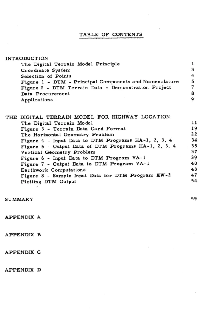
In practice, a convenient data coordinate system is usually es-tablished and is referenced to the master coordinate system. Fi-gure 1, from the MIT DTM System Manual, shows a typical data co-ordinate system, labelled "DTM Coco-ordinate Axes." If the area of interest is rectangular, the x-axis is established parallel to the long dimension of the band. If the area is a square, the x-axis dan be paxallel to any side. The origin is usually located so that the band of interest lies within the first quadrant in order to eliminate the need for negative coordinates.

The question sometimes arises as to why a data coordinate sys-tem is used. This can be answered by stating that there is no

vantage in using the master coordinate system and that the orienta-tion of the master system may not be that desired. The reasons why a particular orientation of the data coordinate system is desirable will become clear in the following sections.

SELECTION OF POINTS

In the definition of the DTM principle, there is nothing said about the distribution of points over the area of interest. In fact, the only restriction on the arrangement of points is that they be recorded in a systematic manner so that they may be easily handled by the com-puter. If the points were recorded in a random manner, the entire set of points, or some portion of it, would bwe to be searched when-ever a particular point was desired.

There are various ways in which the points may be arranged so that they meet the restriction. One such scheme is to record the elevations of points on a fixed x-y grid. This is called the "rigid-grid" system and in the simplest form requires recording only one coordinate, z, for any point once the grid orientation, origin and in-terval are known. The great advantages of this system are the mini-mum amount of data required for any point and the high degree to which data procurement can be automated. The disadvantages are lack of flexibility and the necessity of taking a higher density of points

-4-t

y

State

DIGITAL TERRAIN

MODEL SYSTEM

PRINCIPAL

COMPONENTS AND NOMENCLATURE

Plane Coordinate Axes

for any given accuracy of representation. ("Higher density" refers to other schemes and will be explained in the following paragraphs.)

Another method of arranging the points is to take them along lines parallel to the y-axis. Since these lines have a constant x-co-ordinate, the x-value must be recorded only once for each line. Along a given line (scan line), the points may be taken at constant y incre-ments, constant z increments or variable x and y increments. If either a constant y or constant z increment is used, less data will be required for each line but there will be less flexibility and more points will be required. If a variable y and z are used, more data will be required for each point but fewer points will be taken since

they may be taken at breaks in the terrain. Figure 2, from the MIT DTM Manual, illustrates points taken at uneven y increments on scan lines. As mentioned previously, the less flexible (more rigid) a scheme is, the greater the number of points required compared to a fully flexible system. This also applies to taking the scan lines at variable x increments as opposed to constant x increments.

Another scheme, one that is considerably different from those mentioned above, is to record the x and y coordinates of points along lines of constant z (contour lines). The great advantage of this scheme is that the data procurement would be relatively simple using any one of the x-y recorders commercially available. Though this method is

-6--I

I-D OD

not presently being used, it holds considerable promise for the fu-ture.

Of the schemes mentioned above, the most flexible one (varia-ble x, varia(varia-ble y, varia(varia-ble z) is the one that is presently being used. This does not imply that it is the best method, but rather, indicates that insufficient time has been available to investigate the other schemes.

DATA PROCUREMENT

As stated previously, the data for the DTM is normally taken using photogrammetric methods. The two primary sources of the data are the photogrammetric contour map and the photogramme-tric model itself. In either case the use of special instrumenta-tion can play an important part.

Photogrammetric maps at various scales are generally available and in extensive use in present practice. The DTM sections can be taken from contour maps with very little equipment since all that is needed is a scale to measure the distances. The data is then

tabulated and later translated into computer input material. This means that anyone with a contour map can start taking DTM data immediately. It is obvious, however, that the process of obtaining the great quantities of data necessary for the DTM is tedious and

-8-that some means of improving this process is very desirable. There are various approaches to the problem but the desired instrumentation must essentially be a unit that will measure the y-coordinates of

points and punch or print out the y and z values. Though direct punching is very desirable, a direct print-out is a great advantage over using an engjneer's scale,, manually recording the data, since key-punching the data from tabulations is a relatively simple and fast process. _{When instrumentation which automatically puts the} data on computer input material is used, the problem of data pro' curement is even further reduced. _{One further point should be} men-tioned. _{As the method of obtaining the data becomes more and more} automatic, the opportunities for human error become less. This is a very significant advantage where great quantities of data are concerned.

The second source of DTM data, the stereo model, appears to be the logical place to obtain the data since it is also the source of photogrammetric contour maps. _{However, there are certain factors} which make it unfeasible in many instances to obtain the data direct-ly from the stereoplotter. _{The first important factor is that whereas} contour maps are generally available, stereoplotters are not. This

does not mean that someone who uses maps obtained from a mapping firm cannot also obtain DTM data from their stereoplotters. On the contrary, some of the mapping firms are already furnishing DTM data

on computer input material when so requested. On the other hand, it must also be remembered that at present this is the exception and also that the availability of DTM data does not eliminate the need for maps. The second factor which must be considered when the procurement of data directly from the stereomodel is being weighed, is that the commonly used stereoplotters are designed for producing

contour maps, not cross sections. They are constructed to graphic-ally plot the data obtained from the stereomodel rather than output the information in numerical form. Therefore, in order to obtain cross-sectional data with any efficiency from such a plotter, special

instrumentation must be used. Since the plotters have a means of recording elevations, the minimum additional instrumentation is a device which will measure the y-coordinate. Again, the most de-sirable device is one which will automatically punch out the x, y and z coordinates of points. The important point to remember is that it is not possible to obtain DTM data with only an engineer's scale and a pencil and paper.

APPLICATIONS

The DTM, as described above, is a general principle and is not directly tied to any particular application. The DTM principle

can be used for any problem where numerical calculations involv-ing terrain data are involved. This is particularly true when an area of interest is concerned, such as the area in which an air-port is to be constructed.

The DTM can be very efficiently used in the problem of high-way location since the same set of terrain data can be used to evaluate the earthwork quantities for any number of trial lines. The problem of locating a dam is similar to that of locating a highway though different criteria are used. The DTM can also be applied to this problem. Calculating the volumes of stock piles and borrow pits is another type of problem where the DTM is clearly applicable. Into this category of problems falls that of determining volumes for open-pit mining.

The application of the DTM Principle to the problem of High-way Location is of great interest and importance, particularly be-cause of the impetus given to highway construction by the 1959 Federal Bill creating the Interstate system of roads. This thesis attempts to analyze the steps involved in applying the Digital Ter-rain Model Principle to the problem of highway location using as examples throughout the work done at the MIT Photogrammetry Laboratory.

THE DIGITAL TERRAIN MODEL FOR HIGHWAY LOCATION

Though the Digital Terrain Model is a method of storing terrain data, the Digital Terrain Model System is a combination of the DTM and a group of computer programs to process the DTM data. The DTM principle has been explained in the preceding pages but no mention was made of any computer programs. Therefore, this sec-tion will assume the DTM principle and show what must be done to apply it to a particular problem, highway location. The first por-tion will show what particular form the DTM must take, what co-ordinates are used, and how the data is procured. Various computer programs to edit and process the terrain data will be indicated and an example will be given. Succeeding sections will discuss the various computer programs necessary and the problems involved in utiliz-ing the output from the various programs.

THE DIGITAL TERRAIN MODEL

The problem of highway location is normally concerned with selecting one or more alignments to connect two given points. The problem will vary from that of locating a road to connect two isolated

towns in undeveloped areas to that of revising a portion of some existing alignment. Regardless of the particular problem, one

-11-terion for selecting one alignment over another is the earthwork cost. If the area is uninhabited and the land owned by the agency locating the road, earthwork will be the primary cost. In the case of heavily populated areas, other factors, such as existing structures, will control, However, earthwork will still be com-puted and in no case will be neglected.

Since the area of interest is usually rectangular, the DTM is also usually rectangular. The band of interest will normally nar-row near the ends and may widen in the center portion, Certain parts of it may be eliminated, e. g., it may be decided that under no condition will the road go through a particular cemetery, and there may be regions within the band of interest where no data need be taken. By judiciously examining the area involved, it is often possible to eliminate many regions. Eliminating these areas can greatly reduce the amount of unnecessary data that would otherwise be taken.

The actual size of the band of interest will vary greatly with the phase of the location study.. In a reconnaissance study, the band of interest may be two miles wide with points 100 feet apart. On the other hand, if the final location of a line is desired, the band of interest may be only 1000 feet wide with points averaging

10 to 15 feet apart. Since the actual width of the band and the density of points do not affect the principles involved, no particular

size will be assumed.

For any given project, some direction is normally selected as being that of increasing stationning. The Baseline will there-fore be selected so that it is parallel to the long dimension of the band and so that the Baseline x coordinate increases in the same direction as the center line station. It will also be placed in such a position that all y-coordinates will be positive to eliminate the need for negative coordinates. This, therefore, defines the data coordinate system. Figure 2 illustrates the positioning of a DTM Baseline.

Up to this point it has been assumed that the master coordi-nate system would be a State PlaneCoordicoordi-nate System. Though this will normally be the case, under certain conditions, it may be more practical to use some other coordinate system. Since the choice of master coordinates system has no effect on the DTM principle and since State Plane coordinates are commonly used as master coordinates, the ensuing discussion assumes that the master

system is State Plane Coordinates.

Now that the coordinate systems have been specified, it is well to determine which configuration of points will be used. As men-tioned previously, any arrangement from a rigid grid to a random distribution may be used. For the particular case of highway

-13-I

tion, we will use a system which is similar to the normal practice,

i.e., points will be taken at irregular y intervals along lines of

con-stant x value. (See Figure 2) The DTM cross sections will, there-fore, be similar to right-angle cross sections; points will be taken

at breaks in the terrain along sections and extra sections will be added wherever there is an abrupt change in the terrain between sections. In doing this, the accuracy of the representation of the terrain will be as good as that obtained using normal cross sections. The interval between sections will usually be constant, ranging from 50 feet to 1000 feet depending on the terrain and the accuracy de-sired, and extra sections will be added wherever necessary.

Since the source of this DTM data has not yet been decided

upon, this will now be done. Two sources will be considered: photo-grammetric contour maps and the photophoto-grammetric stereo-model. Though-in some cases data from field surveys may be used with the DTM, this is an unusual case and will not be considered.

Photogrammetric contour maps will be assumed to be the primary source of DTM data since they are generally available and no special instrumentation is required. The stereoplotter will be considered the secondary source, not because it is less suitable, but rather because it, and the associated instrumentation, is less

interchange-4v

-15-ably in the system, and on occasion, the terrain data may come from a combination of both sources. Therefore, the choice of data source does not affect the DTM System.

The process of obtaining DTM data is usually slow and cor-respondingly expensive. For this reason, some mechanical or electronic aids to data procurement are desirable. Before speci-fying what these aids should be, let us examine the steps involved in manually obtaining the data from a map. Given the map, the Baseline must be drawn on it. Next, the cross section lines are drawn perpendicular to the Baseline. Then we are ready to take data. The x value for a cross section is written down and an engineer's scale is used to measure the distance to the first data point. This is recorded. The contour crossing or interpolated elevation at that point is then recorded. This process is repeated until all the data for a section has been recorded. Then a new x value is recorded and the entire process repeated. Since we are assuming the primary storage medium to be IBM cards, the cards must now be keypunched from the data. The cards must then be verified to guard against keypunch errors. We now have our Digi-tal Terrain Model.

The ideal process would merely require the operator to posi-tion an index mark over a point and push a button, punching the

co-ordinates of the point into a card. Such a system would be very desirable, but also very expensive. By examining the manual pro-cess, we can arrive at a solution in between the manual and fully automatic processes that will be adequate and relatively inexpensive.

The actual punching of the cards seems to be a process that can easily be automated, yet it requires that a keypunch be available and that electronic readout circuitry be also available to drive the punch. On the other hand, an experienced keypunch operator can punch great quantities of data from tabalated sheets in a very short time. Since anyone having a card input computer would also have keypunches and keypunch operators available, obtaining the data in neatly tabulated form would not be as inefficient as it first seemed.

Recording the x coordinate of a section need be done only once per section. Therefore, if this step remains manual or semi-manual we have not lost too much efficiency.

The scaling of the y-coordinate and the recording of the y and z coordinates constitute the most tedious portion of the data procure-ment phase. The process is tiring and monotonous and is, therefore,a primary source of error. The basic instrumentation to perform these operations should allow the operator to place the index mark over a point and press a button to print out both the y and z coordinates.

but the z, or elevation, must be at least partially determined by the operator since it is obtained from contour lines. One method of doing this is to take the data points at contour crossings and use a counter to record the contour elevation. The counter could be augmented by the contour interval, remain the same, or be

decreased by the contour interval, depending on the change from the previous point. The operator would then have to push two buttons, one to indicate the change in elevation

(z),

readout the y and z. Such a system, with a few additional refine-ments has been designed and built by the staff of the MIT Photo-grammetry Laboratory and offers great promise as a low cost de-vice for obtaining DTM data.

Once the data has been recorded, keypunched and verified, there are a certain number of operations that may be pe rformed on it. The data can be checked to insure that it meets the speci-fications, e. g., that the points were taken in order of increasing y coordinates. Another operation that may be performed is to alter the card format, e. g. , change the format from 4 points per card to 7 points per card. Still another operation would be to correct an intentional violation of a specification. An example of this would be to record every other section in order of

decreas-ing y coordinates. The advantages of doing this are fairly obvious since the data procurement would become a "back and forth" process

-17-eliminating the need to return to the Baseline before taking the next section. This is particularly useful with automatic readout systems.

Since the data is on punched cards, it is only logical to use the computer to perform the above mentioned operations. The

first DTM computer program to operate in this manner is the Terrain Data Edit program, TD-1; "TD" stands for Terrain Data and will be used to identify all programs which fall into this category. It

is expected that in time, a number of computer programs will be written which will perform all the operations mentioned above and

some whichk-have not yet even been contemplated.

For the series -of programs developed at MIT, the terrain data is stored in the so-called "four per card" format, i. e., each card has the x value of the section and four y-z combinations for four points. Figure 3 shows the card format used for terrain data in the MIT series of programs. A section will, therefore, consist of as many cards as are necessary to contain all the points. The TD-1 program, written by R. A. Baust of the MIT Photogrammetry Laboratory staff, checks the terrain data to ensure that the cross sections are in order of increasing x, the points are in order of increasing y, the x value of points for a cross section agree, the cards are punched in the proper format. When a violation of the

MIT - MDPW - BPR

DTM MANUAL

2-02:

2

8/1/58

DTM TERRAIN DATA

-

IBM CARD TD FORMAT A

(Standard Format for DTM Programs)

Beginning-of-Line Card (one per terrain cross section)

cc

1-5

6-11

12-80

NNNNN

xxxxx.x

Identification Number

DTM x coordinate of the cross section

Blank

Terrain Data Cards (up to four points per card)

NNNNN

xxxxx. x

yyyy.y

szzz.

z

yyyy.y

zzzz. z

yyyy.y

zzzz. z

yyyy.y

zzzz. z

Identification Number

x coordinate

11 punch (identifies card as

Blank (or 11 or 12 punch)

y (offset)

Blank

z (elevation)

Blank

Blank (or 11 or 12 punch)

Blank

cc

1-5

6-11

12

13

14-18

19

20-24

25-29

30

31-35

36

37-41

42-46

47

48-52

53

54-58

59-63

64

65-69

70

71-75

76-80

Blank

z

Blank

terrain data)

First Point

Second Point

Third Point

Fourth Point

Error Designation

-

12 punch in cc 13, 30,, 47, 64 signifies

that the previous terrain point is in error and is to

be ignored by computer.

Partial Card (less than 4 points on a card)

11 punch in

cc 13, 30,

47,

64 signifies that there is

no more

significant data on the remainder of the card.

Punch Requirement

-

card columns 6-11, 14-18, 20-24, 31-35,

37-41, 48-52, 54-58, 65-69, and 71-75 must all be

punched with a number. Use a zero if the number is not

significant. Example, a z of 282' should be punched

as 02820.

-19-Figure 3

Blank

Blank (or 11 or 12 punch)

y

Blank

z

Blank

Blank -(or

11 or 12 punch)

MIT Libraries

Document Services

DISCLAIMER OF QUALITY

Due to the

condition of the original material, there are unavoidable

flaws in this reproduction. We have made

every

effort possible to

provide

you

with the best copy available. If

you are

dissatisfied with

this product and find it unusable, please contact

Document

Services as

soon as possible.

Thank

you.

Pagination error by the author. Page 20

does not exist.

specifications is detected, an error card indicating the type and location of the error is punched. The engineer then uses this information to correct the error. Once the errors have been cor-rected, the data is again processed using TD-1 to insure that no errors were missed and that the corrections were indeed correct.' When the entire deck of DTM data has been processed by TD-1 without detecting any errors, it is then ready for use.

The use of the TD-1 program is explained in the Digital Ter-rain Model System Manual. This manual is divided into three parts: Part I, Engineering Instructions; Part II, Operating Instructions; Part III, Program .nalysis. Part I is intended for the engineer and gives him the information he needs to use the program. It contains no information concerning the actual computer operation nor concerning the program itself since he need not know this in order to use the program. Part II contains the information neces-sary for the machine operator, the person who pushes the buttons and actually operates the machine. This part of the manual con-tains no engineering instructions but essentially tells the operator what buttons to push. Part III contains the information of interest

to the programmer or applications engineer who wishes to under-stand or modify the program. The manual is divided into three parts so that the engineer will not have to wade through much super-fluous information to obtain that which he desires. In a like manner,

-21-the operator will not have to wade through -21-the engineering instruc-tions or the program write-up, nor will the programmer have to go through the engineering instructions. Since the manual has been written in "cook book" fashion, the engineer, operator, or the

pro-grammer, does not have to waste a great deal of time reading be-fore he obtains the information he desires.

Appendix A contains the engineering instructions, operating in-structions and program analysis of the TD-1 program. This write-up clearly shows the form of the DTM Manual and the manner in which it is written.

The importance of this manual cannot be understated. With-out it, _{the programs are useful to no one but the authors.} There-fore, until the instructions for its use are available in a form that makes them easy to understand, the program is practically

value-less. _{The manual is therefore equally as important as the programs}

and the necessary effort should be expended to make it useful.

THE HORIZONTAL GEOMETRY PROBLEM

Horizontal geometry problems are those concerned with the geo-metrical relationships in the x-y plane. _{This includes the basic} pro-blem of relating the data coordinate system to an alignment and also such problems as computing the stationning for points along any given

alignment. As will be seen, certain problems which do not pro-perly belong to this category are included in it for the sake of convenience.

The basic problem in using the DTM for highway location is that of relating a horizontal alignment, defined in the master (State Plane) coordinate system to the terrain data defined in the data co-ordinate system. The data coordinate system is related to the master system by measuring, or computing, the State Plane co-ordinates of the Baseline (x axis) origin and measuring or com-puting its azimuth. This is the information necessary to specify

the rotation and translation of one system relative to the other. The problem therefore reduces to that of determining the intersec-tion of each cross secintersec-tion and the alignment.

The horizontal alignment of a highway is normally composed of tangents, circular curves, and sometimes spirals. This alignment must be mathematically defined so that the intersections may be computed. The tangents may be defined by giving the State Plane coordinates of their intersections (P. I. 's). The circular curves joining the tangents are normally defined in one of two ways: by giving the radius of curvature or by giving the degree of curvature. Either of these two methods of defining a circular curve is accept-able. The spirals are normally used to join the circular curves to the tangents; in the normal case, there would

-23-be a spiral at each end of a circular curve. The spirals are normally defined by giving their lengths. An alignment may there-fore be fully defined by giving the State Plane coordinates of the P. I. 's, the radii of the circular curves, and the lengths of the

spirals. In order to obtain the proper stationning along the alignment, the station of one point, e. g. , the origin, must be given.

Before the intersections of cross sections and the alignment can be omputed, certain other parameters of the alignment must be known. The stations of the T. S. , S. C. , C. S. , S. T. , and the azimuths of the tangents must all be known before any intersection may be computed. This additional data can all be computed from

the data specifying the alignment. These computations can be performed by the computer and since the ansers are also of

in-terest to the engineer, they can be punched out. All this data could be input to the computer, but this would require the engineer to perform calculations which can be performed much more effi-ciently by the machine.

Once the alignment is fully defined, the intersection of the cross sections and the alignment can be computed. This inter-section point is then defined by the center line stationning, the base-line y coordinate and also the skew angle, the angle between the cross

section line and the normal to the alignment at that point. These four parameters are referred to as s, y, and

c//

The problem of computing the intersection can be divided into three parts: (1) Computing the intersection of a cross section and a tangent, (2) Computing the intersection of a cross section and a circular curve, and (3) Computing the intersection of a cross

sec-tion and a spiral. Though the first two are straight forward and can be computed directly, the problem of determining the intersec-tion of a cross secintersec-tion and a spiral is not as simple. The pro-blem reduces to that of solving for the intersection of a straight line (a cross section line) and a third degree curve (approximating a spiral). Though a direct solution to this problem is possible, it appears more feasible to solve by the method of successive approximations.

One or more computer programs are required to solve the problems stated above. These programs and all other programs for this system must meet a certain set of criteria if they are to be a true system, rather than just a series of computer programs. The main criterion that the programs must meet is that they be compatible. They must be developed and written bearing in mind that they are part of an overall system. The IBM 650 computer, for which the first series of programs were written, requires that

a control panel be used in the input-output unit to regulate card formats. _{Rather than have a separate control panel for each} pro-gram, as may easily occur, all, or as many as possible, of the programs should be written so that they use the same control panel. Since the output of some programs will serve as input to others, this should be kept in mind so that the cards punched as output may be used as input without any intermediate processing. The

preci-sion of all the programs must be geared to the same level so that one program does not compute centerline stationning to the nearest tenth of a foot while thepogram which will use this data carries all computa-tions to the nearest thousandth of a foot. Though it may not be feasi-ble to keep the scaling in all programs exactly alike, some effort at uniformity must be made. _{The procedure for using the programs must} be as uniform as possible so that an entirely different operating procedure

is not required for each program. _{The writeups for all the programs} must follow the same general outline so that it will be simple for the engineer or operator to obtain the desired information. By keep-ing all these thkeep-ings in mind it becomes a simple matter to develop an integrated systen of programs, each of which can be easily used once the system is known.

Now that the criteria all computer programs must meet have been stated, it must be decided what computer programs are re-quired to solve the horizontal geometry problem. The first

pro-gram needed is one which can be called the Basic Horizontal Align-ment Program. This program should solve the basic problem of relating the cross sections to a particular alignment.

Input data to this program will fall into two categories, the ter-rain data information and the horizontal alignment information. The terrain data information would be a combination of the DTM cross sections and the data relating the data coordinate system to the mas-ter system. This data would be: Xo and Yo, the State Plane coor-dinates of the Baseline origin, and 9, the azimuth of the Baseline. The alignment data, for an alignment composed of tangents and cir-cular curves with symmetrical spirals, would be as follows: Xi, Yi, the State Plane Coordinates of the alignment origin; Xi, Yi, the State Plane Coordinates of each of the P. I. 's; Xn, n, the State Plane Coordinates of the alignment terminus; Ri, Li, the radii of the circular curves and the lengths of spirals (if a curve has no spirals Ls = _{0); and So, the centerline stationning at the origin of the}

align-ment.

The computations would also fall into two categories: the com-putations to determine the various parameters of alignment geometry such as stationning and azimuths, and the computations for each cross section.

The input data defines the alignment with the minimum

-27-tion necessary. There still remain many parameters which the engineer needs and which he would normally have to compute by hand. Since the necessary information is available to the compu-ter, various parameters are computed, saved for use in the cross section computations, and also punched out so that they are avail-able to the engineer. This information consists of the azimuths of the tangents, the stationning of the T. S. , S. C. , C. S. , and S. T. for each curve, t he distance from the P. I. to the T.S. and S. T. of each curve , the intersection angles of the tangents, and various other constants for each curve.

Each cross section must be related to the alignment by com-puting the baseline y-coordinate of the alignment intersection, the centerline stationning at the intersection, and the angle between

the cross section and the alignment or the tangent to the alingment at that point. This set of data must be computed for each cross section and this is done once the alingment parameters have been computed. One additional piece of data is computed for each sec-tion, the terrain elevation at the centerline. This is easily ob-tained by linear interpolation and provides the engineer with a centerline profile he can use to select the vertical alignment.

The above program, in addition to providing data from which a profile can be drawn, also provides information for plotting a

MIT Libraries

Document Services

DISCLAIMER OF QUALITY

Due to the condition of the original material, there are unavoidable

flaws in this reproduction. We have made every effort possible to

provide

you

with the best copy available.

If you are

dissatisfied with

this

product

and find it unusable, please contact Document Services as

soon

as possible.

Thank you.

Pagination error by the author. Page 29

does not exist.

plan view of the alignment relative to the baseline. The baseline will serve as the reference for plotting the outputs of nearly all

the programs in the system, and will therefore provide a common denominator for all these outputs.

Since it is often desirable to plot right-of-way limits and some-times shoulder lines, the basic program can be modified to compute, in addition to the data for the intersection of each cross section and the alignment, the y coordinate of the intersection of the cross

section and each of two offset lines. If the offset distance corres-pond to the right-of-way distance, the output could be used to plot this line. If the offset distance corresponded to the distance from the centerline to the shoulder point, this shoulder line can be

plotted. If, in addition to computing the y-coordinates of the inter-section of -the cross inter-section and the offset lines, the program also computed the terrain elevation at this intersection, this data would provide the engineer with information about the slope of the terrain in a direction perpendicular to the alignment at each section. Such information would be useful in selecting the grade line.

Another version of the basic program would be one which would compute only the alignment geometry. This vould not be a true DTM program since no cross sections would be involved, but it would provide the engineer with a general purpose program he could use

to check the alignment before using the basic horizontal alignment program.

Still another modification of the basic program can be used to generate data for plotting purposes without using the terrain data deck. Such a program would compute the intersection of the align-ment and scan lines at constant intervals along the Baseline. In-stead of taking the x value from cross sections and using this value to compute the intersections, the program would take an initial value of x, determine the intersection of a scan line having that x value with the alignment, increment the x value by a given interval, demine the intersection, and keep repeating this process until the ter-minus was reached. The alignment could then be plotted with ref-erence to the Baseline. There would be two main advantages to such a program: (1) The terrain data deck would not be used, and (2) The interval used to increment x could be given any value, in-dependent of the cross section spacing. The main drawback would, of course, be the lack of a profile. However, since the program would be used only to generate data for plotting purposes, this draw-back would be of no consequence.

There are many variations of the basic program possible and each would have its own particular application. As the system be-comes more commonly used and experience using it is gained, new

-31-applications and problems are discovered. For this reason, the number and type of programs desirable will not remain constant but will grow with the system. The programs and variations in-dicated above are those which appear desirable from a theoretical standpoint and are basic to the system.

The first set of horizontal alignment programs for the DTM were developed at the MIT Photogrammetry Laboratory. They con-sist of a basic horizontal alignment program, a variation to include offset lines, and a variation to compute the geometry only. In addition to these three, a, straight line interpolation routine was written to obtain profile elevations on even stations.

The DTM Basic Horizontal alignment program, called HA-1, is very similar to the ideal program already described. The main difference is that the HA-1 program uses a horizontal alignment composed only of tangents and circular curves; no spirals are al-lowed. This is not as great a drawback as it would first appear since in location work the inaccuracies introduced by approximating spirals by combinations of circular curves are not significant. Therefore, for purposes of location study, where alternate lines are being compared, there is no great advantage in using spirals.

The input to this program is the terrain data deck; the Base-line Data Card containning Xo, Yo (The State Plane Coordinates

of the Baseline origin) and 0 (the azimuth of the Baseline); the ho-rizontal alignment definition cards containning Xi, Yi (The State Plane Coordinates of the alignment origin, terminus and each P.I.), and Ri (the radius of each circular curve). Figure 4 illustrates the input data neded.

The program computes the geometry of the alignment and punches out the centerline station of the P. C. 's and P. T. 's, the azimuths of the tangents, the intersection angles and the tangent

distances. For each cross section, the program computes and punches out the centerline station, Sx, the Baseline y-coordinate of the intersection of the alingment and the section, and the angle be-tween the section and a normal to the alignment at this point. The program also interpolates for and punches out the terrain elevation at the centerline. _{Figure 5 illustrates the output of the program.}

This program serves as the basic horizontal alignment pro-gram and except for its inability to handle spirals, fulfills all the requirements of such a program. It is expected that with time, this program will be revised to include spirals.

In addition to the basic program, two variations of it have also been written. _{These two variations correspond to the two} mentioned in the previous discussion. The program to com-pute only the geometry of the alignment has been written as

-33-(d) HA-3

Offset Distance

Terminus

(XY)

P.I.1

(X,Y,

R)-

terline

,-VQParallel

Offset Lines

---- P. I.n

(XYR)

Origin

(X,Y,S)

( )

Input Data

S

Station

A

Azimuth

R

Radius of Curve

X,Y

State Plane Coords.

Baseline Origin

(X

,Y)

DTM HORIZONTAL ALIGNMENT PROGRAMS

INPUT DATA TO DEFINE

HA-

1,3,4

EACH TRIAL ALIGNMENT

Fig. HA-I

(A)

Eacti Curve (HA- 1,3,4)

SPT

Station of

T

Tangent

PC and PT

Length

I

Deflection Angle

A

Azimuth of Tangent Ahead

and HA-3)

S

Centerline Station

y

Offse t

Centerline- (HA-1)

z

Ground

and

Elev.

Offset Lines- (HA-3)

DTM HO

OUTPUT

RIZONTAL ALIGNMENT PROGRAMS HA-1,3,4

DATA FOR EACH CURVE AND CROSS SECTION

Fig. HA-2

(Cos

4/)

has the variation to include offset lines. Since these two variations are nearly identical with the programs described previously, they will not be gone into. The input and output of these two programs is shown on Figures 4 and 5.

Appendix B contains the program analysis for HA-1, HA-2, HA-3 and HA-4 and in addition to illustrating the functions performed by the programs, shows their complexity.

The problem of selecting the horizontal alignment has intrigued engineers for many years. In the past, and presently, the horizontal alignment of a road is selected by an engineer using maps, profiles, photographs and various other aids. Since the advent of electronic computers, much interest has been aroused in using the computer to select the best, or "optimum", line. Though many factors enter into the location problem, earthwork in many instances is the prin-cipal or at least an important factor. For this reason, the pro-blem of selecting the best line on the basis of earthwork has been studied. Since there is only one criterion, the problem appears relatively simple. _{However, no satisfactory solution has yet been} obtained. _{The DTM Principle presents an ideal method of storing} the terrain information and, using a high speed computer, the pro-blem may not be too far from a solution. The research in this field is continuing and before too many years, a solution should be forth-coming.

VERTICAL GEOMETRY PROBLEM

Once a trial alignment has been related to the cross sec-tions and fully defined in the horizontal plane, there still remains the problem of selecting a grade line, or vertical alignment. The horizontal alignment program computed for each cross section

the cenerline station, S; the baseline y offset;y; for the intersection of the alignment and the section. One more factor remains to be computed before the earthwork volumes can be calculated, this is the profile elevation for each cross section, Z . The computation of this elevation is the vertical alignment problem.

The vertical alignment program must compute Zp and add it to the output of the horizontal alignment program. The input to the program will therefore consist of the data defining the profile and also the output of the horizontal alignment program. The output will consist of the value Zp added to the input data for each cross section. As mentioned previously, this vertical alignment program is one of a series, and as such, must be an integrated portion of the system. It must accept as input the output from the previous pro-gram and be consistent with it as much as possible. It is possi-ble to compute Zpby conventional methods 2or using a program which is not integrated into the system. However, if this is done, the systems approach to the problem is lost and many sources of error are introduced.

-37-The basic vertical alignment program must take as input, data defining the vertical alignment and compute the elevation Zpfor each cross section. If the vertical alignment is composed of grades and parabolic curves, it may be defined in a number of ways. Pro-bably the simplest way, and the one that will be used, is to define the profile by giving the station and elevation of the origin, termi-nus, and V.P.I.'s and the lengths of the parabolic curves. The other parameters, such as the grades and stations of V.P.C.'s and V. P. T. 's will be computed.

The program will therefore compute two different sets of data, one for the parameters such as grades and curve data, and one

set for the cross sections. The curve data to be computed con-and

sists of the grades of the tangent section and the station/elevation of the V. P. C. 's and V. P. T. 's. Once this is done, the alignment is fully defined. As stated previously, the con terline elevation,

Zp for each cross section will be computed.

In the MIT series of DTM programs, the basic vertical align-ment program is called VA-1 and isessentially that described above. It takes as input data the station and elevation of the origin, ter-minus, and V. P. I. 's and the lengths of vertical curves; in addition to this data defining the vertical alignment, it also takes as input data the cross section output data of the HA-1 program, i.e. for each section: x,

s,

MIT Libraries

Document Services

DISCLAIMER OF QUALITY

Due to the condition of the original material, there are unavoidable

flaws in this reproduction. We have made every effort possible to

provide you with the best copy available. If you are dissatisfied with

this product and find it unusable, please contact Document Services as

soon as possible.

Thank you.

Pagination error by the author. Page 39

does not exist.

Each Vertical

Station and Elevation

_{of VPC and}

VPT

Grade Ahead of each VPI

(+g)

(S,z)

VPC

(z) Centerline Elevation for each

I

Terrain Cross Section x Value

DTM VERTICAL

ALIGNMENT

PROGRAMS

OUTPUT DATA FOR EACH

TRIAL GRADE

LINE

Fig. VA-2 ZAL

Curve

(Sz)

(g)

VA-I

c ons is ts of the s tation and e levation of the V. P. C. 'S and V. P. T. 's , the grades, and, for each section, x, s, y, z, z1 and L The data

for each section is punched on one card and contains all the data re-quired for each section in addition to the terrain data for earthwork computations once the template has been defined. Figures 6 and 7 illustrate the input and output of the VA-1 program. Appendix C contains the program Analysis of the VA-1 and VA-Z programs illustrating the basic logic of these two programs.

The output of the HA-1 program contains for each section the station and terrain elevation of a point on the centerline. Taken together, these points form a profile which is used by the engineer in selecting a trial vertical alignment. The problem of selecting a vertical alignment is much simpler than that of selecting a horizon-tal alignment. For this reason, much work has gone into attempts to have the computer select the grade line. The computer must be given a certain set of conditions to meet before a useful profile can result. The maximum allowable grade must be specified, as must the maximum rate of change of grade. Otherwise, the resulting profile may be acceptable mathematically but completely unacceptable from an engineering standpoint due to excessive grades or insufficient sight distances. There should also be the flexibility of specifying certain control points through which a profile must pass since there are usually interchange or bridge restrictions to be met.

-41-eM

The engineer, in selecting a grade line4 is essentially performing a smoothing process. He tries to pick a profile which meets the given specifications, such as maximum allowable grades, and which will yield the minimum balanced earthwork.

A program has been developed at MIT which attempts to select a grade line based on the terrain profile and certain engineering specifications. _{This program is called the Automatic Profile Design} Program, VA-3. The program selects the profile by using a "least-squares" fit of a third degree polynominal to the terrain for a speci-fied distance ahead of the point in question. The input to the

pro-gram is the output of the HA-1 propro-gram and the engineering informa-tion. The engineering information consists of length of the range ahead to be used, the maximum allowable grades, the maximum allowable rate of change of grade, and the location and elevation of control points to be met, if any. The output of the program is a profile elevation corresponding to each input point. The alignment is there-fore defined by the station and elevation of a great number of points and not by tangents and parabolic curves. Since the program is a radi-cal departure from current practice, extensive testing using a number of different types of data is under way. The results to date have been encouraging and it seems that automatic profile design will soon be a reality.

The selection of a grade line is only one step in the overall au-tomatic highway design problem. It has been the first portion of the problem attacked because it appears to be the simplest. Any tech-niques or programs developed will eventually be incorporated into the overall design program when this becomes feasible.

EARTHWORK COMPUTATIONS

Once an alignment has been defined, both horizontally and vertically, the earthwork quantities can be computed, Earthwork computations are a standard and important problem. In the DTM System, the problem

is basically the same and the same considerations apply. One big decision which must be made is that of selecting the accuracy of computation. If design, or "pay," quantities are desired, the compu-tations will be very precise and detailed. On the other hand, if the study is in the reconnaissance stage, the computed quantities can be fairly approximate without detracting from their usefulness. The intermediate case is that of preliminary location where reconnaissance quantities are not sufficiently accurate and design quantities are not warranted. Of course, design quantities can be used for all three

cases, but in two of them, they would involve unnecessary work and computer time. For this reason the problem of earthwork computa-tions is broken down into three categories: reconnaissance, preliminary

-43-and design.

A reconnaissance earthwork program must provide a means of rapidly evaluating the earthwork quantities for a great number of trial lines. Since the earthwork volumes will be used to evaluate the relative merits of alternate lines, they need not be absolutely but only relatively accurate and since a great number of lines will be evaluated, the computations must be relatively simple. Some reconnaissance earthwork programs use as input data only a terrain profile and assume that the terrain is level on both sides of the centerline. This provides a simple method for computing volumes but does not take into account the cross slope of the terrain. Since a side-hill condition is very common in highway location, the re-connaissance program should take into account the tenain slope, if this can be done without unduly complicating the computations. A solution to this would be to use a two point section. The computa-tions would again be fairly simple and would take into account the terrain slope. The difficulty with this solution is that if one point is on the centerline, the other must be to one side, leaying the other side without a defining point. On the other hand, if the ter-rain points lie on either side of the centerline, there is no center-line profile to use for selecting the grade center-line.

A further refinement is to use a three point terrain section, one point at the centerline and one.on either side. The computations are slightly more complicated but still basically simple. In the DTM