HAL Id: hal-01148822
https://hal.inria.fr/hal-01148822v2
Submitted on 7 Jan 2015
HAL is a multi-disciplinary open access
archive for the deposit and dissemination of
sci-entific research documents, whether they are
pub-lished or not. The documents may come from
teaching and research institutions in France or
abroad, or from public or private research centers.
L’archive ouverte pluridisciplinaire HAL, est
destinée au dépôt et à la diffusion de documents
scientifiques de niveau recherche, publiés ou non,
émanant des établissements d’enseignement et de
recherche français ou étrangers, des laboratoires
publics ou privés.
Realistic Plant Modeling from Images Based on
Analysis-by-Synthesis
Jérôme Guénard, Géraldine Morin, Frédéric Boudon, Vincent Charvillat
To cite this version:
Jérôme Guénard, Géraldine Morin, Frédéric Boudon, Vincent Charvillat. Realistic Plant Modeling
from Images Based on Analysis-by-Synthesis. 8th International Conference on Mathematical Methods
for Curves and Surfaces (MMCS 2012), Jun 2012, Oslo, Norway. pp.213-229,
�10.1007/978-3-642-54382-1_12�. �hal-01148822v2�
Realistic Plant Modeling from Images based on
Analysis-by-Synthesis
Anonymous
Paper ID 019
Abstract. Plants are essential elements of virtual worlds to get pleas-ant and realistic 3D environments. Even if mature computer vision tech-niques allow the reconstruction of challenging 3D objects from images, due to high complexity of plant topology, dedicated methods for gen-erating 3D plant models must be devised. We propose an analysis-by-synthesis method which generates 3D models of a plant from both images and a priori knowledge of the plant species.
Our method is based on a skeletonisation algorithm which allows to gen-erate a possible skeleton from a foliage segmentation. Then, a 3D genera-tive model, based on a parametric model of branching systems that takes into account botanical knowledge is built. This method extends previous works by constraining the resulting skeleton to follow hierarchical organ-isation of natural branching structure. A first instance of a 3D model is generated. A reprojection of this model is compared with the original image. Then, we show that selecting the model from multiple proposals for the main branching structure of the plant and for the foliage improves the quality of the generated 3D model. Varying parameter values of the generative model, we produce a series of candidate models. A criterion based on comparing 3D virtual plant reprojection with original image selects the best model. Realistic results obtained on different species of plants illustrate the performance of the proposed method.
Fig. 1. On the left, an original image of a vine plant before and after a metric rec-tification. In the middle, a possible architecture of the branching extracted with our skeletonisation method. At the right, a 3D model of this plant.
1
Introduction
Procedural methods to generate plant models allow to build a complex plant architecture from few simple rules [1]. For example, Lindenmayer in [2] is a pioneer by proposing the formalism of L-systems as a general framework. By carefully parameterising these rules, it is possible to achieve a large variety of realistic plant shapes [3, 4]. However, a strict recursive application of rules leads to self-similar structures and thus, to enhance realism, irregularities may be gen-erated through probabilistic approaches [5, 1]. Adjusting stochastic parameters to achieve realistic models requires intensive botanical knowledge [6]. Another approach consists in modeling plant irregularities as a result of the competition for space between the different organs of the plants [7]. In this case, the volume of a plant is specified by the user and a generative process grows a branching struc-ture with branches competing between each other. Competition can be biased to favor certain types of structures. However, automatic control of competition parameters to achieve a given shape is still complicated.
All these first works are derived from computer graphics community. Other approaches use also information provided by images to increase the degree of realism. A couple of research directions should be investigated. Clearly, a plant should follow the biological property of its species and also ressemble a picture of an existing instance. That is typically the subject of our work. Our idea is not of exactly reconstructing the plant from an image, including its hidden parts (which seems impracticable) but that of driving the instantiation of the plant 3D model by minimising the difference between its reprojection and the original plant in the image.
Unlike existing methods detailed in section 2, ours must be able to get a 3D model of a plant without any human interaction from images with possibly no visible branches. By integrating biological knowledge of the plant species, we propose a simple fully-automatic process to extract the structure of a plant from the shape of its foliage in a picture taken with as few restrictions as possible and so which may be of poor quality (for example, in the vine case, the image is degraded after a metric rectification du to the assumption that all the principal branches are contained in a same plane as shown at the left on the Fig. 1). We start by presenting a new skeletonisation algorithm in section 3 in the vine case (as we can see in the middle of the Fig. 1) and we explain a possible extension to our skeletonisation method for other kinds of plants with 3D branching architec-ture in section 3.5. Then a 3D model is generated thanks to our 3D generative model (section 4). Finally, an analysis-by-synthesis scheme allows to improve this reconstruction insuring that the foliage model reprojection matches closely the original foliage like explained in section 5 (right on the Fig. 1). The last section shows results and validation comparing with data provided by experts.
2
State of the art: generating plants from images
Realistic plants are challenging objects to model and recent advances in auto-matic modeling can be explained by the convergence of computer graphics and
computer vision [8]. We start this state of the art with the first method of plant modeling from images. Then, we continue with the ones starting by reconstruct-ing clouds of 3D points. After, we talk about other methods usreconstruct-ing several images to finish with approaches using a single image as ours.
A pioneering work on the reconstruction of trees from images was made by Shlyakhter et al. [9] who reconstruct the visual hull of the tree from silhouettes deduced from the images. A skeleton is computed from the hull using a Medial Axis Transform (MAT) and is used as main branches. Branchlets and leaves are then generated with an L-system. The skeleton determined from the MAT does not necessarily look like a realistic branching system. Also, the density of the original tree is not taken into account.
Quan et al. [10, 11] and Tan et al. [12] also use multiple images to reconstruct a 3D model of trees or plants. In order to avoid the features correspondances in different images, they use views close to each other (more than 20 images for any plants). Thus, they obtain a quasi-dense cloud of points by structure from motion. For simple plants, a parametric model is first fitted on each set of points representing a leaf. They then generate branches based on information given by the user. For trees, they start by reconstructing visible branches to create branch pattern that they combine in a fractal way until reaching leaves. Reche-Martinez et al. [13] propose another reconstruction from multiple images, based on billboards. Neubert et al. [14] construct a volume encompassing the plant in the form of voxels using image processing techniques and fill it with particles. Particles path toward the ground and a user given general skeleton are used as branching system.
Wang et al. [15] model different species of trees using images of tree samples from the real world which are analysed to extract similar elements. A stochastic model to assemble these element is also parameterized from the image and make it possible to generate many similar trees. The goal in this case is not necessarily to reconstruct a specific tree instance corresponding to an image. Similarly, Li et al. [16] propose a probabilistic approach to reconstruct a tree parameterized from videos. For these methods, the only source of information is the given images leading to template branching patterns. If the set of patterns is rich enough, it will produce aesthetically pleasing results, but without garantee to be representative of its species. Additionnally, user input are required to specify a draft of the structure on the image to avoid segmentation. Talton et al., in [17], propose to fit a grammar-based procedural methods using Markov Chain Monte Carlo technique to model objects from a 2D or 3D binary shape. Their results are aesthetically very convincing but optimization of their models requires long computation time.
Other approaches explore the use of a single image [18, 19]. In [18], an outline of the plant in the image is determined interactively to extract a skeleton. A 3D representation of the branches is consequently deducted from visible parts, then the leaves are added. Here, an user sketching step is required. In [19], a graph topology is first extracted from a single image of a branching system (a
tree without foliage). Then the 3D tree model is reconstructed by rotating the branches. account too strong constraints about the plants.
In general, methods of the litterature, such as [12] and [18] require visible branches to learn about the structure of the skeleton. In our case, branches are directly from foliage structure. Indeed, the branching structure devised manually by experts from image show that the branches are deduced on one hand from the knowledge of a space filled by a branch and its attached leaves and on the other hand the silhouette of the foliage (left on Fig. 16 on a vine example). We propose a generalised recursive skeletonisation algorithm together with an analysis-by-synthesis mecanism to determine the branches and their attached foliage that is the 3D model. Our approach is fully-automatic, that is, does not require any user interaction.
3
Skeletonisation
3.1 General field skeletonisation method
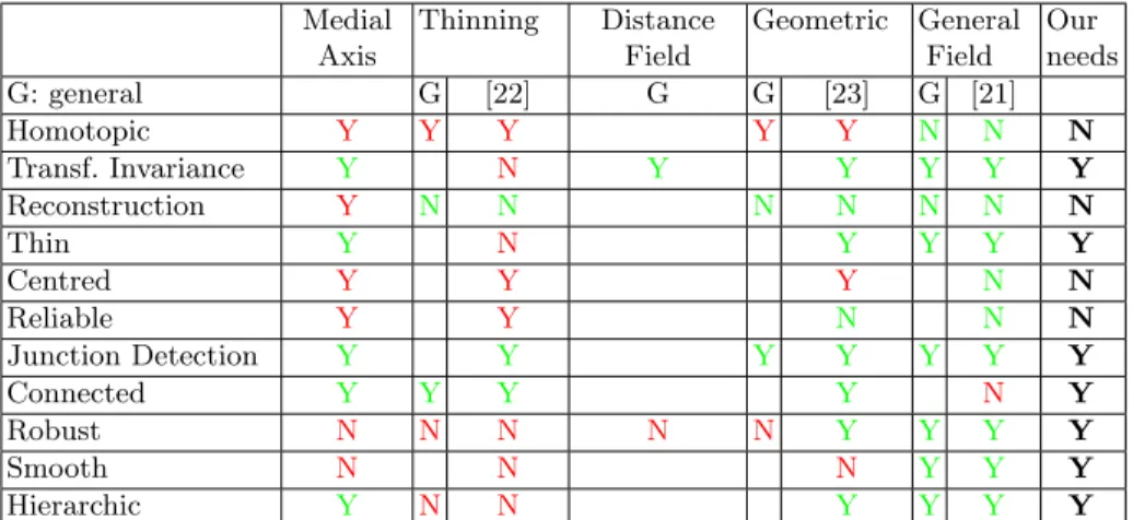
Skeletonisation is a classical topic in image processing. We have followed and completed the analysis of different approaches as proposed in [20] and as illus-trated in Tab. 1. This table summarises the different properties that skeletons respect like the thinness or the robustness and compares them to our require-ments shown in the left column. All these properties are detailed in [20].
In our case, the smoothness is very important to get realistic branches but we do not need a centred skeleton. Morever, the connectivity is less important because it can be ensured by an other way. For these reasons, we choose to adapt the general field method, and in particular the work of Cornea [21], since their approach fits the best our needs.
Medial Axis Thinning Distance Field Geometric General Field Our needs G: general G [22] G G [23] G [21] Homotopic Y Y Y Y Y N N N Transf. Invariance Y N Y Y Y Y Y Reconstruction Y N N N N N N N Thin Y N Y Y Y Y Centred Y Y Y N N Reliable Y Y N N N Junction Detection Y Y Y Y Y Y Y Connected Y Y Y Y N Y Robust N N N N N Y Y Y Y Smooth N N N Y Y Y Hierarchic Y N N Y Y Y Y
Table 1. Summary of properties achievable by different skeletonisation methods. In green, the characteristics compliant with our needs.
Cornea et al. original method [21] consists in computing the skeleton (Fig. 2 (c)) from a vector field (Fig. 2 (b)). For each interior pixel pi of the binary
shape B, a force vector−→fi is computed as a weighted average of unit vectors to
the boundary pixels: − → fi = X mj∈Ω 1 ||−−−→mjpi||2 −−−→ mjpi ||−−−→mjpi||
where Ω contains the contour pixels mj of B (Fig. 2 (a)). Then, points where
the magnitude of the force vector vanishes, so-called critical points (Fig. 2 (b)), are connected by following the force direction pixel by pixel. The results of this method can be seen in Fig. 2. The problem here is that this method is not robust to the holes in the binary shape. Furthermore, sometimes only one branch grows when two or more are required.
(a)
(b)
(c)
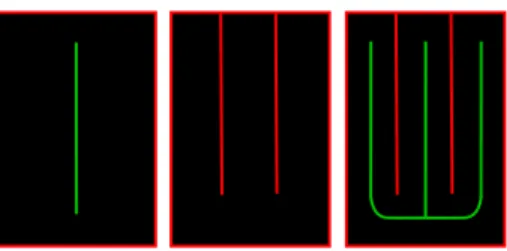
Fig. 2. Cornea et al. original method. (a) shape B with contours pixels ∈ Ω represented in red. (b) vector field with critical points in blue. (c) extracted skeleton in green.
3.2 A new computation of the vector field
By redefining the set of contour points, we manage to use Cornea’s vector field method to get a realistic skeleton in 2D.
Based on botanical expertise, we assume that different branches of relatively similar size coexist and share the space of the crown of a plant. A large convex silhouette may in fact be the sum of all this branching system. For the skeleton reflects this hierarchy of branches, we propose a strategy to partition silhouette space into subsets by positioning artificial contour points in the shape. Fig. 3 shows that by adding contour points within the shape, we define an appropriate branch set.
We compute a probability map P on B containing, for each interior point pi, the probability to be considered as a contour point. The new force vector
− →
fi
does not depend only on the points mj∈ Ω but on all the points of B. The new
formula to compute the vector field is: − → fi = X mj∈Ω 1 ||−−−→mjpi||2 −−−→ mjpi ||−−−→mjpi|| + X pj∈B\Ω j6=i Pj ||−−→pjpi||2 −−→ pjpi ||−−→pjpi|| (1)
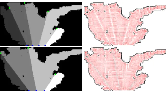
Fig. 3. At the left, the skeleton (in green) extracted with Cornea’s original method. A spatial partition can be generated (red lines) to constraint skeleton computation to a more branched shape. At the right, the skeleton computed by Cornea’s method when all red points are considered as contour points.
We can see that if Pj = 0 for all the interior points, we find Cornea
for-mula whereas the points with a high probability act as a repulsive force on the positioning of the branches.
3.3 Definition of the probability map
We assume here that n the number of branches is given. We compute the prob-ability map P with an iterative algorithm. The first step is the choice of cuts in B. The cuts are segments with one starting point and one ending point and represent the possible positions of the separations between the n branches in the shape. Assuming that the shoots grow vertically from the cane, we propose to place trivially the ending points ei, i = 1..n − 1 of the cuts uniformly in the
bottom of B (Fig. 4). Then, the starting points are computed one by one. To do that, we compute the DCE (Discrete Curve Evolution) of Ω as in [24]. It provides a simplified polygonal boundary composed of N vertices (sl),l=1..N like
shown in Fig. 5. Usually, we choose N = 2n. An angle αlcan be associated with
each vertex, representing clockwise angle between the 2 segments around the vertex. A set of points (ck),k=1..K uniformly discretises the polygon.
Then a new probability ρk to be a starting point is computed for each point
ck taking into account two values:
– the proximity to an inward angle:
ρ1k ∼ N X l=1 1 d(ck, sl) (1 − αl 2π)
– the distance along a boundary to the set H of already chosen starting points: ρ2k ∼ min
c∈Hd(ck, c).
The mix probability ρk is proportionnal to φ(ρ1k, 1, σ) + φ(ρ2k, 1, σ) where
φ(., 1, σ) represents the gaussian function with a mean equals to 1 and a standard deviation equals to σ (here, σ = 0.4).
Fig. 4. At the left, examples of cuts with n = 4 and n = 5 branches. Ending points are represented in blue and starting points in green. At the right new vector fields.
Fig. 5. DCE algorithm examples. At the left, the original image with the contour points around the foliage. The two other images show the DCE algorithm with a 24-point polygon in the middle and a 8-24-point polygon on the right. The inward angles are represented in blue.
A starting point {ck} is selected according to the probability ρk. Then it is
associated with an ending point eiand accepted if:
#pixels ∈ B on the lef t of (eick)
#pixels ∈ B − i n ≤ τ (2)
where τ is a parameter allowing the created partitions of the binary shape to have the same size or not. In the vines case, τ = 15%.
Finally, when all the cuts have been accepted, the new vector field is com-puted like shown at the right part of Fig. 4.
3.4 Adjusting first order branches
We now have a vector field coherent with the n branches assumption. We want to extract branches from this vector field. For each row i of the image and each area p of the partition that we can see at the left part of Fig. 4, we extract the attracting point api which is the one with the smallest vector norm. Each branch bpis a Catmull-Rom curve adjusted on the attracting points api, using a least
square criterion.
Fig. 6. A final skeleton with 5 branches.
The following algorithm summarises the proposed approach: ALGORITHM:
input: binary shape B and number of branches n.
output: a skeleton model of the plant consisting in n branches.
∗ Compute the DCE of B with N = 2n vertices and extract candidate {ck}
uniformly along the polygon. ∗ Initialise H = ∅.
∗ Place the ending points {ei, i = 1..n − 1} in the bottom of B.
∗ For i from 1 to n − 1 · Compute ρk for each (ck).
· while (!equation (2))
◦ Randomly select a starting point c among {ck}\H in function of ρk and
an ending point among {ei}.
· H = H ∪ c.
∗ Compute the probability map P.
∗ Compute the vector field using equation (1).
∗ Extract the points api for each row i of each area p of the partition. ∗ Ajust a branch in each area p of the partition.
∗ For each node of each branch, extract a foliage width.
3.5 Higher order branches and depth information
In the case of the vines, all the main branches are assumed in a same plane and there are only first order branches. We adapt this planar setting to a more recursive structure and to a 3D setting where rotational symmetry is assumed, like in typical monopodial plants (i.e. plants organised around a main trunk).
Automatic colour based segmentation extracts the 2D binary shape of the foliage. Then, the branches are extracted using a modified version of our algo-rithm presented above. The ending points are placed on the vertical line passing through the trunk of the monopodial tree and the condition (2) is replaced by a condition checking that the angle between the cut and the trunk is coherent (i.e. around π2 in the bottom of the tree, π6 in the top and with an angle computed linearly between these two values for an intermediate cut). This algorithm is applied recursively to get second order branches for each partition. We can see an example of cuts with a Liquidambar tree in Fig. 7.
Fig. 7. An exemple of skeleton for the Liquidambar tree.
Depth of branches
To generate 3D information, we drew inspiration from Zeng et al. [19] and Okabe et al. [25]. The goal is to deduce depth information for the branches in the 2D skeleton to make a realistic plant from other views, preserving the appearence from the original viewpoint as it is shown in Fig. 8. First, we compute the convex hull of our 2D skeleton. Then, revolving this convex hull around the line passing through the trunk, we obtain a encompassing volume of the plant. Considering an orthographic projection onto the ground, for each branch which does not touch the 2D convex hull, we change depth information for that the end of this branch touches the boundary of the bounding volume. We have two possibilities, at the front or at the back. We choose the one which maximises the angles between the projections of all the branches to the ground, adding the branch one by one.
Fig. 8. At the left, we can see the 2D convex hull of the foliage, in the middle, the-bounding volume and at the right, the final 3D skeleton of a Liquidambar tree.
4
3D Generative Model
Now we have a possible structure of the plant, the next step is to generate a 3D model of this plant. To do that, we need to build a 3D generative model thanks to all the a priori knowledge of the plant.
In our work, we combine procedural methods to generate a plant and image based approaches. Procedural methods makes it possible to take into account botanical constraints such as possible regular arrangements of organs (for in-stance leaves). The procedural model uses stochastic parameters in the position-ning of the branchlets and the leaves.
We choose to generate the constrained model with systems, using the L-Py modeller [26]. An L-system [1] is a formal grammar, most commonly used to model the growth processes of plant development. The main idea of L-systems is to rewrite a string of modules representing the structure of the plant. Rewriting rules express the creation and change of state of the various modules of the plant over time. Our model include a deterministic part which is controlled by the understanding of plant images and a stochastic part to allow a more realistic result. The model is deduced by both learning from a large number of plants and also knowledge given by specialists.
We choose to generate our model in two stages: the branching system model and the foliage.
Branching system model
Each branch is set by a number of 3D nodes which are the control nodes of the branch. From each of these nodes one or more lateral branches of the same nature may grow. Then, to model the 3D structure, each branch is a generalised cylinder along a curve passing through all nodes. A B-Spline curve is built with a local interpolation scheme of degree 3 [27]. A radius is assigned to each of these nodes to determine the radius of the generalised cylinder in these nodes. This radius is linearly interpolated between two nodes. Textures taken from real images are then applied to branches.
Foliage model
We begin by extracting leaf textures from real images. At each node defining the branches structure is also assigned a value R which is the radius of the cylinder encompassing the leaves. Thus, to model the foliage, branchlets are generated randomly along the branches. Stems are placed along main branches and branchlets. Their density and their length is a random variable distributed normally with mean R and standard deviation R
4. On each of these stems a leaf
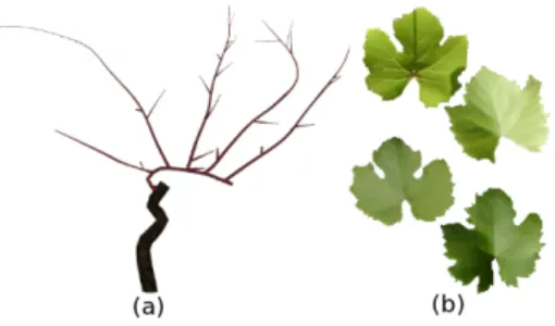
modeled by a Bezier surface is placed on which a randomly chosen texture is mapped (Fig. 9b.).
5
Reprojection criterion
The last step goals to evaluate the quality of the 3D reconstructed 3D model. We reproject the 3D model in an image with the same viewpoint of the original image. We obtain a binary shape Ii (1 if foliage, 0 elsewhere). In the same
Fig. 9. Example with the case of vine. (a) Branch structure modelisation. (b) Textures of vine leaves.
way, the original segmented foliage forms a second binary image B. The error reprojection is computed as:
errori=
#((Ii− B)2== 1)
#pixels(B) (3)
Fig. 10 illustrates the comparison between the projections and the original image.
Fig. 10. At the left, the original image. At the right, the reprojected model. In the middle, the projection errors map. White pixels correspond to pixels where the original image and the reprojected one are superposed and red pixels are wrong pixels.
The idea now is to improve the proposed 3D model using an analysis-by-synthesis strategy which allows to merge information from the a priori botani-cal knowledge and from the image. An increasing number of authors propose to use external knowledge for easing reconstruction from images. Indeed providing knowledge about the scene to be reconstructed simplifies the image processing steps. In [28], Tu et al. define generative models for faces, text, and generic regions which are activated by bottom-up proposals learnt using probabilistic methods. These proposals are then accepted or rejected using a stochastic cri-terion. Yuille et al. [29] claim that this approach, which allows to deal with the complexity of natural images, has intriguing similarities to the brain. They present a method where low level features are used to make bottom-up pro-posals, finally validated by high-level models. In a similar analysis-by-synthesis method where a priori knowledge consists in geometric and mechanical
proper-ties, Gupta et al. [30] iteratively make proposals for interpreting parts (blocks) of the image. We use a similar approach, but not iterative.
In our case, we give more freedom to the generative model. For example, we do not impose the number of branches of the plant that we do not a priori know. Thanks to all the knowledge of the plant, we can model each parameter (like the position of the cuts, the leaves densities or the number of branches) by a random variable, and thus generate numerous models.
We select the best candidate proposed by the generative model using the following formula: Mi0 = argmax Mi p(Mi|Ii) = argmax Mi p(Mi)p(Ii|Mi) (4)
We choose p(Ii|Mi) = 1−errori= 1−
#((Ii−B)2==1)
#pixels(B) and p(Mi) is a product
of terms which are probabilities function of all the knowledge of the plant. For the vine case example, one of the term of p(Mi) is a gaussian representing the
probability of the number of shoots. Fig. 11 shows different error maps. White pixels correspond to pixels where the reprojected model and the original image are superposed.
Fig. 11. Different errors maps with different numbers of branches, different distribu-tions of leaves and different densities. The map outlined in red is the error map of the selected 3D model because there is the smallest percentage of gray pixels.
6
Results and Validation
Our method has been tested on a large number of images and videos. Some results are shown in Fig. 15, 14 and 12. To validate our model, a criterion which can be used is the error given by the equation (3). The average error for the case of vines is 6.9%, 7.2% for the Walnut and 8.5% for the Liquidambar. In Fig. 13, we show the reprojection error according to the number of tested models for an example of vine (the third example of Fig. 12). It is interesting to note that
the greater is the number of tested models, the lower is the reprojection error. The curve decreases very quickly between 1 and 15, fairly quickly until 100. This proves the effectiveness of our skeletonisation method which restricts significantly the search space. This curve illustrates the importance to test several models but of course, the final selected model is not necessarily the last one.
Fig. 12. Vine plants modelisation. At the top the original images. At the bottom, rendering of automatically generated vine models using our approach.
A second validation is to compare our solution to the one provided by viticul-ture experts (Fig. 16). It seems difficult to find a significant measure by compar-ing the ground truth to our skeletons. Furtheremore, for us, the most important is the final appearence with leaves. Indeed, for the first example in Fig. 16, our algorithm found a very similar skeleton to the expert one at the left but it is not the one which has been validated by our method at the right. So, we used our algorithm on the drawn ground truth skeletons with different leaves distribu-tions and different leaves densities to find the best 3D model. The improvement of the reprojection criterion in comparison to our automatically generated skele-ton is only 0.2% in average. This small difference proves the performance of our method which does not require human intervention.
In Tab. 2, we can see the number of shoots drawn by two differents experts from vines images. The last row shows the number of shoots of the 3D models generated with our method from the same images. We almost reconstruct a 3D model with the same number of shoots drawn by one of the two experts.
For the 3D case, we have shown that our method can reconstruct realistic 3D trees from a single image. However, the branching system is mostly based on branches.
number of tested models 1 model differ en t n um ber s o f br a nc h es 1 lea ves dis tribu tio n 1 lea ves den sity differ en t n um ber s o f br a nc h es differ en t leaves dist ribu tion s 1 lea ves den sity differ en t n um ber s of br a nc h es 1 lea ves dis tribu tio n differ en t leaves den sit ies differ en t n um ber s o f br an ches differ en t leaves dist ribu tion s differ en t leaves den sit ies er ro rs on t h e r epr oj ec ti on c riter io n (% )
Fig. 13. Reprojection errors according to the number of tested models. Different varia-tions are tested as the number of branches or the leaves density. For example, if we test different 3D models with only one leaves distribution and 1 leaves density, the error is almost 10%. Then, this error decreases when we add different leaves distibutions or different leaves density.
Image 1 2 3 4 5 6 7 8 9 First expert estimation 3 6 5 5 6 5 3 7 7 Second expert estimation 2 6 4 5 4 4 2 5 4 Our method 2 5 4 5 6 6 3 5 6
Table 2. The first row represents the number of the vine image. The second and the third rows represent the numbers of shoots drawn by the experts. The last row represent the number of shoots of the 3D models generated with our method from these images.
7
Conclusion
Combining analysis and sythesis, we have proposed a new fully-automatic method of plant modeling from a low resolution image without any branching pattern unlike [12, 19].
The leading contribution of this paper is a new skeletonisation algorithm able to extract the structure of a plant from an image of its foliage. Then, we built 3D parametric generative models for different plants using the knowledge about the species. A final analysis-by-synthesis step improves the quality of the final 3D model by comparing the original image with a large number of 3D models generating varying different parameters of the 3D generative model.
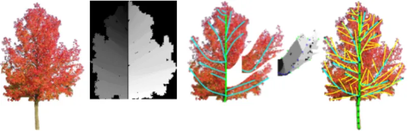
Fig. 14. Walnut. At the left, the original image. At the right, the 3D model with the same viewpoint.
Fig. 15. Liquidambar. At the left, the original image. In the middle, the 3D model with the same viewpoint. At the right, the 3D model with an other viewpoint.
The skeletons are used to make proposals to the 3D generative model. The reprojection criterion insures the similarity between the proposed 3D model and the original image. We further validated our proposed model by comparing it to ground truth given by experts in the case of vine.
In future work, we could investigate the automatisation of the use of a priori. Indeed, the construction of the generative model could be done by learning from a large data set avoiding the necessity prior knowledge on the branching structure of the plant species. The process would be evolving in loop, where the analysis could give feedback to the generative models.
References
1. Prusinkiewicz, P., Lindenmayer, A.: The algorithmic beauty of plants. Springer Verlag (1990)
2. Lindenmayer, A.: Mathematical models for cellular interaction in development: Parts i and ii. Journal of Theoretical Biology 18 (1968)
3. Weber, J., Penn, J.: Creation and rendering of realistic trees. In: Proceedings of the 22nd annual conference on Computer graphics and interactive techniques. SIGGRAPH ’95, New York, NY, USA, ACM (1995) 119–128
Fig. 16. Expert skeletons. At the top, a viticulture expert has drawn skeletons on vine images (in red). At the bottom, the projections of the skeletons of our method (in yellow).
4. Deussen, O., Lintermann, B.: Digital Design of Nature: Computer Generated Plants and Organics. Springer-Verlag (2005)
5. de Reffye, P., Edelin, C., Fran¸con, J., Jaeger, M., Puech, C.: Plant models faithful to botanical structure and development. In: Proceedings of the 15th annual con-ference on Computer graphics and interactive techniques. SIGGRAPH ’88, New York, NY, USA, ACM (1988) 151–158
6. : Markov and semi-markov switching linear mixed models used to identify forest tree growth components. Biometrics (2009)
7. Palubicki, W., Horel, K., Longay, S., Runions, A., Lane, B., Mˇech, R., Prusinkiewicz, P.: Self-organizing tree models for image synthesis. SIGGRAPH (2009) 1–10
8. Quan, L.: Image-based Plant Modeling. Springer (2010)
9. Shlyakhter, I., Rozenoer, M., Dorsey, J., Teller, S.: Reconstructing 3d tree models from instrumented photographs. IEEE Comput. Graph. Appl. (2001) 53–61 10. Quan, L., Tan, P., Zeng, G., Yuan, L., Wang, J., Kang, S.B.: Image-based plant
modeling. ACM TOG (2006) 599–604
11. Quan, L., Wang, J., Tan, P., Yuan, L.: Image-based modeling by joint segmenta-tion. IJCV (2007) 135–150
12. Tan, P., Zeng, G., Wang, J., Kang, S.B., Quan, L.: Image-based tree modeling. ACM TOG (2007) 87
13. Reche-Martinez, A., Martin, I., Drettakis, G.: Volumetric reconstruction and in-teractive rendering of trees from photographs. ACM TOG (2004) 720–727 14. Neubert, B., Franken, T., Deussen, O.: Approximate image-based tree-modeling
using particle flows. ACM TOG (Proc. of SIGGRAPH) (2007)
15. Wang, R., Hua, W., Dong, Z., Peng, Q., Bao, H.: Synthesizing trees by plantons. Vis. Comput. 22(4) (April 2006) 238–248
16. Li, C., Deussen, O., Song, Y.Z., Willis, P., Hall, P.: Modeling and generating moving trees from video. ACM Trans. Graph. 30(6) (December 2011) 127:1–127:12 17. Talton, J.O., Lou, Y., Lesser, S., Duke, J., Mˇech, R., Koltun, V.: Metropolis
18. Tan, P., Fang, T., Xiao, J., Zhao, P., Quan, L.: Single image tree modeling. ACM SIGGRAPH (2008) 1–7
19. Zeng, J., Zhang, Y., Zhan, S.: 3d tree models reconstruction from a single image. ISDA (2006) 445–450
20. Cornea, N.D., Silver, D., Min, P.: Curve-skeleton properties, applications, and algorithms. TVCG (May 2007) 530–548
21. Cornea, N.D., Silver, D., Yuan, X., Balasubramanian, R.: Computing hierarchical curve-skeletons of 3d objects. The Visual Computer (2005)
22. Yang, X., Bai, X., Yang, X., Liu, W.: An efficient quick thinning algorithm. In: Proceedings of the 2008 Congress on Image and Signal Processing, Vol. 3 - Volume 03. CISP, Washington, DC, USA, IEEE Computer Society (2008) 475–478 23. Bai, X., Latecki, L.J., Society, I.C., yu Liu, W.: Skeleton pruning by contour
partitioning with discrete curve evolution. IEEE Trans. Pattern Anal. Mach. Intell 29 (2007) 449–462
24. Latecki, L.J., Lakmper, R.: Shape similarity measure based on correspondence of visual parts. PAMI (2000) 1185–1190
25. Okabe, M., Owada, S., Igarashi, T.: Interactive design of botanical trees using freehand sketches and example-based editing. Computer Graphics Forum 24(3) (2005) 487–496
26. Boudon, F., Pradal, C., Cokelaer, T., Prusinkiewicz, P., Godin, C.: L-py: an l-system simulation framework for modeling plant development based on a dynamic language. Frontiers in Plant Science 3(76) (2012)
27. Piegl, L., Tiller, W.: The NURBS book (2nd ed.). Springer-Verlag New York, Inc. (1997)
28. Tu, Z., Chen, X., Yuille, A.L., Zhu, S.C.: Image parsing: Unifying segmentation, detection, and recognition. In: Toward Category-Level Object Recognition. (2006) 545–576
29. Yuille, A., Kersten, D.: Vision as bayesian inference : Analysis by synthesis ? introduction : Perception as inference. Psychology (2006) 1–15
30. Gupta, A., Efros, A.A., Hebert, M.: Blocks world revisited: Image understanding using qualitative geometry and mechanics. In: European Conference on Computer Vision(ECCV). (2010)