Accurate belief state update for probabilistic constraint automata

by

Oliver Borelli Martin

B.S., Department of Aerospace Engineering California Polytechnic State University, 2002

SUBMITTED TO THE DEPARTMENT OF AERONAUTICS AND ASTRONAUTICS IN PARTIAL FULFILLMENT OF THE REQUIREMENT FOR THE DEGREE OF

MASTER OF SCIENCE at the

MASSACHUSETTS INSTITUTE OF TECHNOLOGY June 2005

@

2005 Massachusetts Institute of Technology All rights reserved.

Signature of Author ...

Certified by ...

Associa

...

Department of Aeronautics and Astronautics May 20, 2005

Brian C. Williams te Professor of Aeronautics and Astronautics

N

1 1 Thesis Supervisor

A ccepted by ... ... ... . Per. aire Professor of Aeronautics and Astronautics Chair, Committee on Graduate Students

AERO

_I

MASSACHUSETTS INSTITUTE OF TECHNOLOGY

JUN 2 3 2005

by

Oliver Borelli Martin

Submitted to the Department of Aeronautics and Astronautics on May 20, 2005, in partial fulfillment of the

requirements for the degree of Master of Science at the Massachusetts Institute of Technology

Abstract

As autonomous spacecraft and other robotic systems grow increasingly complex, there is a pressing need for capabilities that more accurately monitor and diagnose system state while maintaining reactivity. Mode estimation addresses this problem by reason-ing over declarative models of the physical plant, represented as a factored variant of Hidden Markov Models (HMMs), called Probabilistic Concurrent Constraint Automata

(PCCA). Previous mode estimation approaches track a set of most likely PCCA state

trajectories, enumerating them in order of trajectory probability. Although Best-First Trajectory Enumeration (BFTE) is efficient, ignoring the additional trajectories that lead to the same target state can significantly underestimate the true state probability and result in misdiagnosis. This thesis introduces two innovative belief state approximation techniques, called Best-First Belief State Enumeration (BFBSE) and Best-First Belief State Update (BFBSU), that address this limitation by computing estimate probabilities directly from the HMM belief state update equations. Theoretical and empirical results show that BFBSE and BFBSU significantly increases estimator accuracy, uses less mem-ory, and have no increase in computation time when enumerating a moderate number of estimates for the approximate belief state of subsystem sized models.

Thesis Supervisor: Brian C. Williams

Title: Associate Professor of Aeronautics and Astronautics

This thesis would not have been possible without the persistence and patience of Brian Williams, Michel Ingham, and Seung Chung. It has been a privilege to work with you and I appreciate the continuous guidance and encouragement that you have provided me.

To all my family and friends: Please forgive me for my negligence over the past few years. I look forward to spending much more time with everyone in the future.

This research was supported in part by NASA's Cross Enterprise Technology Devel-opment program under contract NAG2-1466, and by the Jet Propulsion Laboratory, through the JPL Director's Research and Development Fund under contract 1261107.

1 Introduction 13

1.1 Previous W ork . . . . 13

1.2 Thesis O utline . . . . 14

2 Decent Stage IMU 17 2.1 Simple IMU Example ... . 18

2.1.1 The IMU Component Model ... ... 19

2.1.2 The Power Switch Component Model ... 21

2.1.3 The Timer Component Model ... ... 21

2.2 PCCA Plant Model ... 22

2.2.1 PCCA Formalism ... ... 23

2.2.2 Example: The IMU System PCCA Plant Model ... 24

3 Estimation of PCCA 29 3.1 Belief State Update ... 29

3.1.1 PCCA Transition and Observation Probabilities ... 30

3.1.2 Example: IMU System Belief State Update . . . . 32

3.2 Optimal Constraint Satisfaction Problems . . . . 35

3.2.1 Example: IMU System OCSP Belief State Update . . . . 37

4 Approximate Estimation of PCCA 39 4.1 Belief State Update Approximations . . . . 39

4.1.1 Exponential Belief State Approximation . . . . 40

4.1.2 Trajectory Approximation . . . . 41

8

CONTENTS

4.1.3 Observation Approximation . . . . 4.2 Best-First Solutions using OPSAT . . . . 4.2.1 Conflict-directed A* . . . .

4.2.2 Estimation using OPSAT . . . . 4.2.3 Example: Most Likely Trajectory for the IMU System . 4.3 Best-First Belief State Enumeration . . . . 4.3.1 BFBSE Heuristic Function . . . . 4.3.2 Example: BFBSE for the IMU Plant . . . . 4.4 Best-First Belief State Update . . . . 4.4.1 Observation Probability Rules . . . . 4.4.2 Offline Generation of Observation Probability Rules 4.4.3 Online BFBSU using Observation Probability Rules 4.4.4 Example: BFBSU for the IMU Plant . . . .

5 Results and Discussion

5.1 Space and Time Complexity . . . . 5.2 Experimental Results . . . . 5.2.1 A ccuracy . . . . 5.2.2 Perform ance . . . . 6 Conclusion 6.1 Summary of Results . . . . 6.2 Future W ork . . . .

A IMU System Constraint Automata Definitions

A.1 The Power Switch Constraint Automaton, A . . . . .

A.2 The Timer Constraint Automaton, At . . . . A.3 Compiled IMU Plant Model Dissents . . . .

B Best-First Trajectory Enumeration

B.1 BFTE Heuristic Function . . . .

. . . . 43 . . . . 45 . . . . 45 . . . . 47 . . . . 48 . . . . 50 . . . . 50 . . . . 52 . . . . 56 . . . . 58 . . . . 60 . . . . 64 . . . . 66 71 71 73 74 77 81 82 82 85 85 87 88 89 90

2-1 Mars Science Laboratory sky-crane EDL . . . . 2-2 Simple IMU system block diagram. . . . . 2-3 Model of IMU operational modes. . . . . 2-4 Model of Power Switch operational modes. . . . . 2-5 Model of Timer operational modes. . . . . 2-6 IMU constraint automaton, Aimu. . . . .

3-1 The Trellis diagram of the possible state evolutions over time. . . . 3-2 Single-step exact belief state update of the IMU Plant. . . . . 3-3 Single-step OCSP exact belief state update for the IMU Plant. . . .

4-1 Belief state probability distribution for a simple IMU Plant scenario. 4-2 Decomposing the belief state evolution into a branching structure. . 4-3 Approximate trajectory propagation for the IMU Plant. . . . . . 4-4 Approximate observation probability update for the IMU Plant. 4-5 Single Trajectory Enumeration for the IMU Plant. . . . . 4-6 Best-First Belief State Enumeration for the IMU Plant. . . . . . 4-7 Iteration 1 BFBSE expansion for the IMU Plant. . . . . 4-8 Iteration 2 BFBSE expansion for the IMU Plant. . . . . 4-9 Iteration 3 BFBSE expansion for the IMU Plant. . . . . 4-10 Iteration 4 BFBSE expansion for the IMU Plant. . . . . 4-11 OPR dependency hypergraph for the IMU Plant. . . . . 4-12 Best-First Belief State Update for the IMU Plant. . . . . 4-13 Iteration 1 BFBSU expansion for the IMU Plant. . . . . 4-14 Iteration 2 BFBSU expansion for the IMU Plant. . . . .

9 18 19 20 21 22 25 30 32 37 41 41 . . . . 42 . . . . 44 . . . . 49 . . . . 52 . . . . 53 . . . . 54 . . . . 55 . . . . 55 . . . . 62 . . . . 66 . . . . 67 . . . . 68

10

LIST OF FIGURES

4-15 Iteration 3 BFBSU expansion for the IMU Plant . ... ... 68

5-1 Probability density maintained over time for EO-1 model . . . . 75 5-2 Probability density maintained over time for the Mars EDL model. . . . 76 5-3 Probability density maintained over time for the ST7-A model. . . . . 76 5-4 Single state estimate probability over time for the ST7-A model. . . . . . 77 5-5 Best-case and average-case runtime performance for the EO-1 model. . . 78 5-6 Best case and average case runtime performance for the Mars EDL model. 79 5-7 Best case and average case runtime performance for the ST7-A model. . . 79

A-1 PS constraint automaton,

Ap. . . . ..

86 A-2 T constraint automaton,

At. . . . .

87

2.1 Aimu Modal Constraints . . . . 25

2.2 Aimu Transition Functions

/

Probabilities . . . . 26

3.1 Enabled Component Transitions for the IMU Plant, P . . . . 33

4.1

Results for Best-First Trajectory Enumeration . . . .

43

4.2 Results for Approximate Observation Probability Update . . . . 45

4.3 Enabled Component Transitions for the IMU Plant, P . . . . 53

5.1 Space and Time Complexity for BFTE, BFBSE, and BFBSU . . . . 72

5.2 Experimental Model Properties . . . . 74

5.3 Number of Observation Probability Rules for each Model . . . . 80

A.1 Ap, Modal Constraints . . . . 86

A.2 A,, Transition Functions

/

Probabilities . . . . 86

A.3 At Modal Constraints . . . . 87

A.4 At Transition Functions

/

Probabilities . . . . 88

Introduction

The purpose of estimation is to determine the current state of the system. An estimator infers the current state by reasoning over a model of the system dynamics along with the commands that have been executed and the resulting sensory observations. In many embedded systems, this knowledge of the current state is then used by a controller to drive the system state towards a specific target or goal. The ability for a system to accurately and reliably deduce its current state can dictate whether it is able to achieve its objectives. This is particularly important for highly complex robotic space exploration systems that operate in uncertain environments. Furthermore, deep space communication delays and severely constrained on-board computing capabilities present tremendous challenges to traditional methods of estimation in support of robust autonomous spacecraft operations.

1.1

Previous Work

Previous work in model-based monitoring and fault diagnosis, including GDE/Sherlock [6, 7], GDE+ [19], Livingstone [21, 15], diagnosis using model-checking [5], and Titan Mode Estimation [20], have made significant advances towards meeting these challenging per-formance requirements. All of these capabilities achieved reactivity, while maintaining reliability, by framing mode estimation as a best-first shortest-path problem, which can be efficiently solved using a variant of the Viterbi algorithm [10]. This approach is known as Best-First Trajectory Enumeration (BFTE) and works quite well when trying to de-termine the "most likely explanation" to a sequence of observations. Livingstone was successfully flight validated on the NASA Deep Space One probe as part of the Remote Agent Experiment in 1999 [17]. Unfortunately, approximating the current state by the

14

INTRODUCTION

most likely trajectory can significantly underestimate the true state probability and re-sult in misdiagnosis. In addition, failure to update the estimates with valid observation probabilities places a probabilistic bias on failure modes, which can drive the estimator towards incorrect fault diagnoses during continuous nominal operations.

This thesis introduces two novel mode estimation techniques, called Best-First Belief State Enumeration (BFBSE) and Best-First Belief State Update (BFBSU), that approx-imate the belief state by generating the set of most likely estapprox-imates and achieve greater accuracy than BFTE by computing the estimate probabilities directly from the Hidden Markov Model (HMM) belief state update equations, instead of approximating them by their trajectory probability. This contribution significantly increases the accuracy of the estimator while using less memory and less computational time; providing an enabling technology for increasingly complex space missions of the future.

1.2

Thesis Outline

This thesis first provides a motivating example of a small IMU system, similar to the one that will fly on the decent stage of the Mars Science Laboratory [12] in 2009. Our Prob-abilistic Concurrent Constraint Automata (PCCA) formalism [21, 20] is then presented in detail and the IMU Plant model is formally described. Chapter 3 reviews the exact solution to the PCCA estimation problem using the HMM belief state update equations, eluding to some practical limitations due to PCCA state space explosion. The PCCA es-timation problem is then framed as an Optimal Constraint Satisfaction Problem (OCSP), providing the framework for efficient best-first enumeration of state estimates. Due to state space explosion, Chapter 4 discusses the three significant approximations that were employed in BFTE to achieve the strict computational requirements of severely con-strained embedded systems, while maintaining estimate accuracy. BFBSE and BFBSU are then introduced as superior mode estimation techniques that significantly improve estimate accuracy through direct use of the HMM belief state update equations. In addition, BFBSE and BFBSU improve estimator performance by framing the PCCA es-timation problem as a single OCSP, and using the observation probabilities in the search

heuristic to quickly identify likely solutions and avoid sub-optimal candidates. In Chap-ter 5, we support our claims of improved estimator accuracy and performance through theoretical and empirical comparisons between BFTE, BFBSE, and BFBSU. Experimen-tal data gathered from three different spacecraft subsystem models show good alignment with our theoretical expectations. In conclusion, Chapter 6 summarizes the technical contributions of this thesis and provides insight into future areas of research in the field of model-based monitoring and fault diagnosis.

Decent Stage IMU

The Mars Science Laboratory (MSL) is NASA JPL's next generation Mars rover, which is currently slated to be launched in December of 2009. The primary science objective of MSL is to conduct in-situ analysis of Martian soil in search for organic compounds that are necessary to support life [12]. MSL is twice as long and three times as massive (3000 kg) as the Mars Exploration Rovers (MER), carrying an unprecedented 10 science instruments. Due to this large size and mass, the current airbag landing system is no longer sufficient and a novel "sky-crane" approach (shown in Figure 2-1) will be used to safely place MSL on the Martian surface. In addition, MSL will be the first Mars Lander to use precision guidance during entry, decent, and landing (EDL), in order to accurately control MSL to within a 10km x 5km, 3- landing target error ellipse [12]. This innovative EDL sequence and precise landing target requirement places a substantial demand on the MSL EDL system, which must operate autonomously due to the 4 to 21 minute time-delay between Earth and Mars.

The Inertial Measurement Unit (IMU) is a critical component for supporting MSL EDL. An IMU is typically composed of 3 accelerometers and 3 gyroscopes, one for each axis, and is responsible for providing body-frame position and attitude measurements with a fast update rate, as necessary for real-time control. MSL will rely on an IMU attached to its decent stage (Figure 2-1) in order to make the necessary adjustments to its flight-path during entry for a safe and precise rover landing. With less than 6 minutes in the entire EDL sequence, quick and accurate monitoring and diagnosis of the IMU operational mode is essential for the success of the mission. Failure to autonomously diagnose and recover from an IMU failure mode would certainly lead to unreliable position

18

DECENT STAGE IMU

y Interface I -I I I I I I I I I I I I I I I I I I I I I I I I I I I I I I I I I I I I I I I I I I I I I I

Deploy Supersonic Chute

Jettison Heatshield, Activate Radar, and Deploy Mobility

Sense Velocity with Radar

Jettison Chute and Backshell, Begin Powered Descent

48. 6s Begin Sky-Crane Maneuver

II

I 33.3s ... Rover

Decent Stage

MSL Rover

Flyaway

Figure 2-1: Mars Science Laboratory sky-crane entry, decent, and landing sequence [12].

and attitude knowledge, followed by imminent mission loss due to a hazardous landing.

Although approximate belief state enumeration is applicable to nearly any embedded

system, the MSL EDL demand for autonomous, responsive, and accurate monitoring and

fault diagnosis, makes the decent stage IMU a highly relevant example that will be used

throughout this thesis. This chapter presents a decent stage IMU system, similar to that

of MSL, that is greatly simplified for pedagogical clarity, but sufficiently complex to

high-light the innovation and importance of the additional accuracy provided by approximate

belief state enumeration. The chapter concludes with graphical models of the IMU and

its accessory components.

2.1

Simple IMU Example

An Inertial Measurement Unit (IMU) is a standard sensor package that is used to provide

spacecraft and other robotic systems with translational and angular motion

ments. Space qualified IMUs are typically radiation hardened and tightly coupled to the spacecraft body; firmly mounted to the rigid-body structure, thermally controlled, and electrically wired to provide two way communication between the IMU and the attitude determination and control (ADC) processor. The IMU system modeled in this thesis is greatly simplified to three interconnected components, as shown in Figure 2-2.

Switch Command

oPower

IMU Data e

Data Valid Flag

IMU Mode Timer Status

Figure 2-2: Simple IMU system block diagram.

This simplified IMU system consists of the basic IMU itself, a controllable Power Switch (PS) that provides the IMU with a power source, and a Timer (T) that is used to help infer whether the IMU has become stuck in an undesirable mode. Although the IMU and PS are interconnected with the data bus, which passes information to the ADC processor, we chose to not model this component for simplicity, and we assume that there is always power flowing into the Power Switch. Detailed descriptions of each component are provided below.

2.1.1

The IMU Component Model

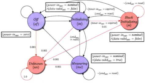
This simple IMU is a relatively passive device that reacts primarily to the input power coming from the Power Switch. During nominal use, the IMU is ready to take measure-ments shortly after an initialization period, which occurs when it is first powered on. Although the main function of the IMU is to provide continuous motion measurements, for the purpose of monitoring and diagnosing the IMU operational mode, we will ignore this data. A graphical representation of the discrete IMU modes are shown in Figure 2-3. The IMU has 5 defined operational modes, 3 of which are considered nominal and

20

DECENT STAGE IMU

(power-in -- nominal) =cmze=reset)

A(d at a-valid,,u = fase utmenm, =exprd

(cdIMu reset)

(timer-inm =ep1 ed

F(power-in zero) ig u (cmd (power-inof= nooninal)

-. me A(data-validess false) 0.001 0.001 apower-in,, = nominal) 0.001 _{A(data-e lidn =csTsi} 0.001

Figure 2-3: Model of IMU operational modes.

2 failure modes. When the IMU first receives power, it transitions from the Off mode

and begins initializing, during which the IMU measurements are not reliable and the

data-valid flag is false. After a short period of time (typically less than 22 seconds), the

IMU produces valid data and is ready for use. If the power is removed from the IMU

at any point in time, it will return to the Off mode. It is also possible for the IMU to

become Stuck Initializing if the Timer expires during the initialization process. This is a recoverable fault mode in which a reset command can be issued to to restart the IMU initialization. It is important to note that, if the IMU has to be reset multiple times, or there are unexplainable sensor measurements of the data validity that contradict the expected IMU behavior, it is more likely that the IMU is in an Unknown mode and the spacecraft should quickly switch to its redundant IMU (not modeled) in order to

recover. The probabilities on the transitions will be explained at the end of this chapter

in Section 2.2.

'For the purpose of this thesis, a failure mode is simply defined as an undesirable mode that is unexpected and rarely occurs (lower probability of occurrence).

2.1.2

The Power Switch Component Model

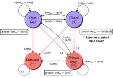
The sole purpose of the Power Switch (PS) is to provide the IMU with power. For the

purpose of this simple IMU system, we will assume that the PS is always receiving power.

An illustration of the PS is shown in Figure 2-4.

-, (cmda = close) -(cmda, = open)

(emd,, = open)

(cmap = close)

(power-out, = zero) (power-out, - nominal)

(cmd * Assumes constant

open) _{input power}

0.0005 0-1

0.0005 0.

0.0005 -,(cmd, = open)

1.0 _{(power-out,s = zero)}

Figure 2-4: Model of Power Switch operational modes.

This Power Switch has 2 nominal modes and 2 failure modes. When the PS is

commanded closed, the switch is shorted and power is supplied to the IMU. Likewise,

when the PS is commanded open, power is removed from the IMU. In the presence of too

much electron current, the PS will become Tripped Open in order to prevent overloading

and possibly damaging the IMU. A safe recovery can be conducted by reopening the

switch and then closing it again to power on the IMU. Similar to the IMU, there is also

an Unknown mode, which captures all other unexpected behavior.

2.1.3

The Timer Component Model

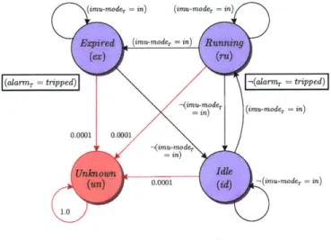
The third component is the IMU Timer (T), shown in Figure 2-5, which is responsible

for keeping track of how much time the IMU has spent Initializing. When the IMU is not

initializing, the Timer is Idle. As soon as the IMU begins initializing, the Timer starts

Running and an external continuous timer starts in the background. When the external

22

DECENT STAGE IMU

Stuck Initializing. Alternatively, if the IMU exits from the initializing mode before the

external timer expires, the external timer will have no effect on this model and will simply

reset the next time the IMU begins initializing.

/' (imnu-moder = in) (imu-moder in)(

(alarMT tripped)j =_aam tripped)]

- (imu-mode,

= in) (imu-mode2. in)

0.0001 0.0001

0.001 -(imu-modeT = in)

1.0

Figure 2-5: Model of Timer operational modes.

This concludes our summary of the three components that constitute our simple

ped-agogical IMU plant. The next section section defines a specific type of factored HMM

modeling formalism that is used in this thesis and provides a formal description of the

sim-ple IMU system. Chapter 3 introduces the comsim-plete PCCA estimation problem, followed

by Chapter 4, describing the challenges that PCCA estimation presents for embedded

systems and assumptions that have made monitoring and fault diagnosis tractable for

full-scale systems.

2.2

PCCA Plant Model

As in previous work, we model the physical plant as a factored Hidden Markov Model

that is compactly encoded as Probabilistic Concurrent Constraint Automata (PCCA) [20].

The PCCA represent a set of concurrently operating components that are interconnected

and interact with their surrounding environment. Each automaton has a set of possible

discrete modes with conditional probabilistic transitions, which capture both nominal and

faulty behavior. These modes are only partially observable, due to a limited number of

sensors, but are inherently constrained by the system properties that define each mode. In this section we review the formal definition of the PCCA plant model and provide an illustrative example using the simple IMU system that was previously introduced in

Chapter 2.

2.2.1

PCCA Formalism

We first define a single probabilistic constraint automaton and then the composition of multiple automata. A probabilistic constraint automaton for component "a" is defined by the tuple Aa = (HaMaTa,Pa):

1. Ha H' U -I is a finite set of discrete variables for component "a", where each

variable 7ra E la ranges over a finite domain D(7ra). fl' is a singleton set containing

mode variable {Xa} =1' whose domain D(Xa) is the finite set of discrete modes in Aa. Attribute variables Hl include inputs, outputs, and any other variables used

to define the behavior of the component. Ea is the complete set of all possible full assignments over Ha and the state space of the component

Ex-

= E4x. is the projection of Ea onto mode variable Xa.

2. Ma : Ea - C(11) maps each mode assignment (Xa = Va) E Ea to a finite

domain constraint ca(Xa = Va) E C(H;), where C(flU) is the set of finite domain constraints over U;. These constraints are known as modal constraints and are

typically encoded in the propositional form A A True I False (u = y)

I

-'A, A, A A2

I

A, V A2, where y E D(u). If the current mode is (x = Va) at time-step

t, then the assignments to each attribute variable rt E H' at time-step t must be consistent with Ca(Xa = Va). These constraints capture the physical behavior of the mode.

3. Ta : E,. x C(U;) -- E is a set of transition functions. The set of finite domain con-straints C(U;) are also known as the transition guards, encoded in the propositional form A. Given a current mode assignment (Xa = Va) E Exa and guard ga C (H )

24 DECENT STAGE IMU

specifies a target mode assignment (Xa = v') E Ej" that the automaton could transition into at time-step t

+

1. Ta = Tn U Tf captures both nominal and faulty behavior.

4. Pa : Ta(Xa = Va, ga) -* W[0, 1] is a transition probability distribution. For each mode variable assignment in Ea and guard gt, there is a probability distribution across all transitions into target modes defined by the set of transition functions Ta(Xa va, ga).

The entire system plant P is modeled by a composition of concurrently operating constraint automata. Each automaton is interconnected to both its environment and other automata through constraints on shared variables. Formally, the PCCA plant model is defined by the tuple P = (AI,Q):

1. A= {A, A2, ... , A,} is the finite set of constraint automata that represent the n components of the plant.

2. 1 = Ua-r..n ra is the set of all plant variables. The variables 1 are partitioned into a finite set of mode variables Um = Ua=1..nrHm, control variables

r*

Ua=1..n

r;,

observation variables _{' C Ua=i.Inr, and dependent variables}

_rd

_{- Ua=l..n a.}

EC, E, and Ejd are the sets of full assignments over Uc, 1", and Id.

3.

Q

C C(rL) is a set of finite domain constraints that capture the interconnections between plant components.

2.2.2

Example: The IMU System PCCA Plant Model

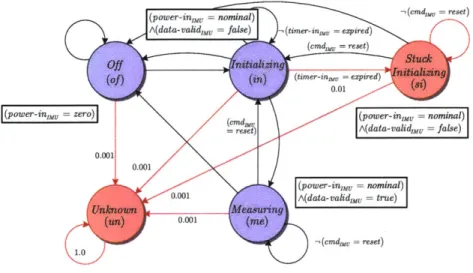
The simple IMU system introduced in Chapter 2 will be used in this section to clarify the PCCA formalism. Our PCCA plant model P is composed of the constraint automata for the IMU (Aimu), Power Switch (Ap,), and Timer (At). As an example of a single constraint automaton, consider the IMU component shown again in Figure 2-6.

(power-in,, = zero)

0.0(

11.0

( power-in,,, = nominal) ,(cmd,,, - reset) A(data-valid,,, = false) ,(timer-in,,, = expired)

{cmda. = reset) (timer-injmu = ezpired)-! - 0.01 (cmd~ (power-insyy = nominl

i

A(data-validmyy = false) .001 (power-inu = nominal) 0.001 A(data-vald ue

O

(cmda, = reset)

Figure 2-6: IMU constraint automaton,

Aimu.

1.

[Iim

_1IMu

= {Ximu, _{X mu} pm _{iu oM Im imu I} dv dP, di :} where {ximu} =rImm resides in 1 of 5 discrete

_{resde in}

modes D(ximu) =

{

of, in, me, si, un} as indicated with circular nodes in Figure 2-6. HIrm =

{I4m,

oq'nu, dnu,

dri} where

prnd

is used to reset the IMU with D(pg d)

= reset, no-commandv, oq is an observation of the data validity with ID d(o d) =

{true, false}, di is the power-in with D(di) = {zero, nominal}, and d." is a

time expiration variable with D(diu) =

{expired,

not-expired}. Eimu =Eu X

Emu is the set of all full assignments over

Himu

with 5 - (2 . 2 -2 -2)

=

80 elements.

2. Mimu includes the constraints encapsulated by rectangles in Figure 2-6. The

com-plete set of modal constraints for the IMU are shown in Table 2.1 below.

Table 2.1:

Aimu

Modal Constraints

(Ximu =

Vimu)

E

G;X;

Mimu(ximu

=

vimu)

imu Km~ximu=

ero

) Ximu =

of

ximu = in ximu = me ximu = si ximu = un dmu = zero

dt = nominal A oq' =

f

alse

= nominal A o = true = nominal A oq' =

f

alse

(unconstrained)

3. The component transitions are indicated by the arrows and labels in Figure

26 DECENT STAGE IMU

{I

, Tn2, Tf

}

where (Ximu = si) is the source mode and (Ximu = in), (Ximu = of),

and (Ximu = un) are the target modes. The complete set of transition functions for

Aimu are shown in Table 2.2 below.

Table 2.2: Aim, Transition Functions

/

Probabilities

(zimu =vimu) Ximau of Ximu Ximu Ximu Ximu Ximu Ximu Ximu

in

in

me

me

Si st un gimu E C(TImu) (unconstrained) -,(df = expired)

di'mu =expired

(p = reset) ymucim = reset

_,

_{= reset)}

cmd _reset (unconstrained)

Timu( ximu = vimu, gimu)

{

of, in, un}

{of,

in, me, un}

{of,

me, si, un}

{of,

me, un}

{of,

in, un}

{of,

si, un}

{of,

in, un}

{un}

PTip(Ximu = Vimu, gimu)

{0.4995, 0.4995, 0.001} {0.333, 0.333, 0.333, 0.001} {0.4945, 0.4945, 0.01, 0.001} {0.4995, 0.4995, 0.0011 {0.4995, 0.4995, 0.001} {0.4995, 0.4995, 0.0011 {0.4995, 0.4995, 0.001}

{1}

4. The component transition probability distribution for each set of IMU transition functions is shown on the right side of Table 2.2 above.

For completeness, the formal definitions to Aps and At are listed in Appendix A. The full PCCA plant model for this simple IMU system is composed of 3 components and the interconnections between them. The power output of the PS is connected to the power

input of the IMU and the T is connected to the IMU to help determine if the IMU has become Stuck Initializing2. The PCCA plant P for the IMU system is formally defined

as follows:

1. A ={Aim, Aps At} is the set of all constraint automata in the IMU system; including the IMU, Power Switch, and Timer.

2. 1 = im U H , U lUt is the set of all variables. This set is partitioned into mode

2

The transient initialization process of the IMU is a perfect example of when a Timed Plant Model

[13] would be preferred over a PCCA to increase the fidelity of the model. Since this thesis is limited

to only PCCA models, we have compensated for the continuous-time IMU behavior by introducing a discrete Initializing mode for the IMU as well as a Timer component, that interacts with an external continuous timer, to help determine if the IMU is Stuck Initializing. Although the concepts of Best-First Belief State Enumeration in this thesis are presented in the context of PCCA, the method could be expanded to improve the accuracy of Timed Mode Estimation.

variables 1' = {xim, zps,X t}, control variables 1c {p9"', pcmd}, observation variables

H

= o I}, and dependent variables Id = i, d dPj, d"}.

3. The interconnections for the IMU system are

Q

Ximu - dttmA

d t= d

J

where the power-out (po) of the PS is connected to the power-in (pi) of the IMU, the IMU mode variable Ximu is connected to imu-mode (im) of the T, and the T mode variable xt is connected to the timer-in (ti) of the IMU.

With the PCCA formalism defined, the next chapter will introduce the full PCCA estimation problem as well as approximations that are used to make the problem scalable to full-sized systems.

Estimation of PCCA

This chapter reviews exact belief state update for PCCAs and presents a formulation of the estimation problem as an Optimal Constraint Satisfaction Problem (OCSP), inter-leaving examples using the IMU system. The task of estimation is to calculate a belief state of the system in real-time, while maintaining accuracy and reliability. A belief state is a probability distribution over the states of a system, which represents the likelihood of the system being in any single state, given a history of past commands and observations. For PCCA, a state si is defined as a full assignment to mode variables si

e

zm and a belief state B = (S, p) is a finite set of estimates that cover all consistent states S C Em . Each estimate consists of a state si E S and its posterior probability p(si) E p.

3.1

Belief State Update

The Markov property declares that the future state of a system is conditionally inde-pendent of its past, given its current belief state. This property allows an estimator to iteratively compute the next complete belief state Bt+1 at time-step t + 1 by only considering the current belief state Bt and commands At at time-step t, along with the resulting observations o+1. The belief state is then computed using the standard HMM belief state update equations [1):

P(s +1 0<oat> <Ot>) (p(,t+1 tp oo> <o't-1>))(31

stESt

P(st+1 <Ot> <Oxt>) . p(6t+1|st+1)

P(s+ 3 <41 t+1a (t1i ₍₃₁ 2),>p

Es Et+1 P(si+ I~a> I~a)po+ i 1

30

ESTIMATION OF PCCA

Equation 3.1 represents the a priori probability of being in the next state sj+1 at

time-step t + 1, given all the observations oOt> and commands p<0't> between time-step

0

and t. P(sf|oCO't>, p<o't1'>) E pt is the probability that the system was in state si at

time-step t and P(s

1

s , A) is the state transition probability. Equation 3.1 propagates

the system dynamics into the future before considering new observations. Once all the a

priori estimates are generated, Equation 3.2 then updates these estimates by adjusting

the probabilities based on new observations o+1 using the Total Probability Theorem

and Bayes' Rule to calculate the a posteriori probabilities

pt+1

across all states in St+1.

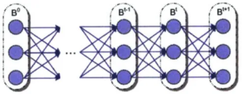
The belief state evolution over time can be visualized in a Trellis diagram, as shown in

Figure 3-1. Each column represents a separate belief state at different time-steps. Arrows

depict conditional dependence between states, and correspond to transitions between

states. The probabilities associated with each state in the belief states are not shown.

Figure 3-1: The Trellis diagram of the possible state evolutions over time.

3.1.1

PCCA Transition and Observation Probabilities

To complete the definition of belief state update for PCCA, the state transition

proba-bilities and observation probaproba-bilities must be defined. Since the PCCA are concurrently

operating, the state transition consists of a set of component mode transitions; one mode

transition T for each component (Xa = Va) E si. By assuming that each component

tran-sition is conditionally independent given the current state si and commands pt, the state

transition probability simply becomes the product of the component transition

proba-bilities (Equation 3.3). This assumption, previously made by Livingstone [21], has been

demonstrated in practice to be reasonable for a wide range of engineered systems.

P(s'+1 8,t) =

17

+1 _{v'Ix' = Va, 8, pt)) (3.3)} The component mode transition probability P(xz+1 = xz = Va, s, y') is the

prob-ability of transitioning from mode (x = Va) at time-step t to mode (xz+ 1 = va) at the

next time-step, conditioned on the current state of all components si and commands yt. Recall from the PCCA formalism that if transition guards ga are entailed by si and yt, the set of transitions Ta(Xa = va, ga) are considered to be enabled and their target modes are reachable; otherwise the transitions are disabled with a transition probabil-ity of zero1. To be probabilistically complete, the sum of the enabled outgoing state transition probabilities must be 1 for each s E Bt.

The conditional observation probability P(ot+1|s+) is the probability of sensing ob-servations o E E', given that the system is in state si E Em at time-step t

+

1. For PCCA, the observation probability distribution is defined using a consistency approach similar to that of GDE [6], such that for every state sj E Em

, there is a probability distribution across all combinations of observations. If every observation 01 E ot+1 is entailed or refuted by the conjunction of the modal constraints M and state s+ 1 , the

observation probability P(ot+1 s+1) is 1 or 0, respectively. When the observations are neither entailed nor refuted, there is a uniform probability distribution of 1/m across all the m possible consistent values of ot+1, creating a probabilistic bias towards states that predict (entail) observations. This uniform distribution assumption is a degener-ate case of Maximum-Entropy [14] when there is no previous knowledge about how the sensors behave. The precise observation probability distribution for PCCA is shown in Equation 3.4.

1 if s'+1 A M ot+1, P(ot+llst+l) = 0 if st+1 A M -,ot+1,

i j _(3.4)

/m otherwise,

where m = number of consistent assignments to ot+1 for sj+ 1 and M.

1_{0n rare occasion, it is possible to have a transition guard that is neither entailed nor refuted,}

resulting in a probability that the transition is enabled. This is beyond the scope of this thesis but is discussed as future work in Section 6.2.

32

ESTIMATION OF PCCA

3.1.2

Example: IMU System Belief State Update

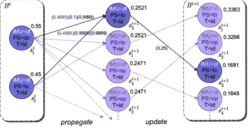
The simple IMU system described in Section 2.1, and formally defined in Section 2.2, is now used to demonstrate the mechanics of the propagate and update equations that were introduced in Section 3.1. This example uses the belief state update equations to compute the exact solutions to the PCCA estimation problem. Figure 3-2 illustrates a single estimation cycle where the belief state update equations first propagate the IMU system dynamics to calculate the a priori state probabilities (center of Figure 3-2) and then update those estimates with the resulting observation data to determine the a

posteriori state probabilities (right of Figure 3-2). The labels on the arrows represent

the component transition probabilities (one for each component) during the propagation step, and observation probabilities during the update step. Due to the large state space of this simple example2, only the leading four estimates are shown for Bt+1.

0.25210.3363

(0.4995)(0.1)(0.9999 0.55 3+1 (0.4995)(0. (0.9999) 0.25 _0.3296 0.2471 _0.1681 0.45 0 1 648 propagate update

Figure 3-2: Single-step exact belief state update of the IMU Plant.

Given the current belief state Bt, consisting of s' with probability 0.55 and s2 with probability 0.45, we will focus on the process of generating the state probability for s'3+,

as highlighted in Figure 3-2. Assuming that there are no commands pt and only consistent

2_{Since all of the components are independently operating, the actual number of estimates contained} in the full belief state is Hyker| D(yk)|, where yk contains only the reachable mode assignments of xt+1

such that D(Yk) C D(xt+1). Recall that a mode is reachable if there is an enabled component transition

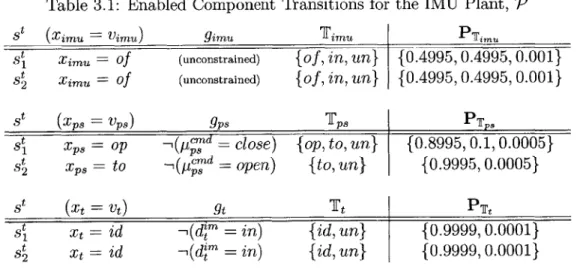
observations ot+1, both current states have enabled state transitions that converge to a single next state +1 with an a priori probability of 0.2521. This state is then updated with its observation probability to result in an a posteriori state probability of 0.1618. Before we can calculate the a priori state probabilities, we must first determine all the enabled component mode transitions by determining which transition guards are entailed. The enabled transitions and their probabilities for all three components of the IMU system are shown in Table 3.1 below:

Table 3.1: Enabled Component Transitions for the IMU Plant, 'P

st (Ximu Vimu) gimu Timu PTsm

71 zimU= of (unconstrained) {of, in, un} {0.4995, 0.4995, 0.0011

2s Ximu = of (unconstrained) {of, in, un} {0.4995, 0.4995, 0.001}

st (x,8 = vp.) gps Tp PTP,

s , = op , d - close) {op, to, un} {0.8995, 0.1, 0.0005}

s2 z = to ,(p = open) {to, un} {0.9995, 0.0005}

st (Xt = Vt)Tt PTt xt = id xt = id (d" = in) ,1(dm = in) {id, un}

{id, un}

{0.9999, 0.0001} {0.9999, 0.0001}

Now we can compute the state transition probabilities by taking the product of the enabled component transition probabilities. Since we are interested in state st+1, we will only consider the state transitions leading to the target state {Ximu = of, xP, = to, Xt id}. The probabilities for the two state transitions that converge to state s'+1

are computed below:

P(3Isi, pt) = P(Ximu = of IXimu = of)P(x,, = tolxz8 = op)P(xt = idIxt = id)

- (0.4995) (0.1) (0.9999) - 0.049945

P(s=+1 p(imu = (t) Of IXimu = of)P(x,, = toIx, = to)P(xt = idixt = id) - (0.4995) (0.9995) (0.9999)

- 0.4992 t

Si

34 ESTIMATION OF PCCA

Using the belief state update propagate equation from Equation 3.1, we can now calculate the a priori state probability by multiplying each state transition probability by their originating state probability and then summing over all the incoming transitions into state s3+1

P(st+1io<o't> g<o,t>) __p t+1 st lt p ,t o<o,t> g,<o,t-1>)

+

P(s+1 It , fit)P (s1 0 <O,t> 1 <O,t-1>)

= (0.049945)(0.55) + (0.4992)(0.45) = 0.2521

This is the same a priori state probability shown in Figure 3-2. The next step is to update this probability with the resulting observations ot+1 using Equation 3.2. In this example, we have assumed that we received observations that are consistent with s.+1, By reconciling the modal constraints of the IMU automata defined in Chapter 2.2 and Appendix A, there are four unique sets of observation assignments that are consistent with both st+1 and M:

{ol', = true, o1 _{= tripped},}

{oiU - true, ol = not-tripped}, {od =

f

alse, o" = tripped , {o =

false,

of = not-tripped}.

Since a set of observations is neither entailed nor refuted, the observation probability for state s+1 is P(t+11 5 +1) = 1/4 = 0.25 (as shown in Figure 3-2), where there are 4

consistent sets of observations. This observation probability is then used in Equation 3.2 to compute the a posteriori probability as shown below:

P~st+1o~o~t1> g

~Pt>

3+1 o<o,t> <o,t>) . p(Ot+|s+1

33 O~s +1Es++1 10 o>o<Ot>><o=t> 11 s +1)

(0.2521)(0.25) (0.37487) 0.1681

summing over the all posterior probabilities for belief state Bt+1 prior to normalization. For this example, the normalization factor is 0.37487.

This completes the belief state update for state s3+1. In order to compute the full belief state, this same process must be completed for all 18 possible reachable states in Bt+1. It is important to note that although st+1 and st+1 are more likely than ss+1 in Bt-+ (as illustrated in Figure 3-2), the IMU cannot be Initializing while the Power Switch is Tripped Open or Open, since the Power Switch does not supply the IMU with power in either of those modes3. Due to our factored model representation, belief state update alone will not eliminate these inconsistent states. A solution to this problem is presented in the next section by framing the estimation problem as an Optimal Constraint Satisfaction Problem (OCSP) [22]. Using this framework, a solution is only valid if all the constraints are satisfied, hence, inconsistent states st+1 and s'+1 are invalid solutions and would not be returned.

3.2

Optimal Constraint Satisfaction Problems

PCCA estimation can be viewed as a problem of constraint optimization, where each reachable target state st+1 in the belief state Bt+1 must be consistent with modal con-straints M, component interconnections

Q,

and observations ot+1. This constraint op-timization formulation was previously used in Titan [20] and can similarly be used to formulate the methods underlying GDE [6], Sherlock [7], and Livingstone [21, 15]. This thesis leverages a similar OCSP formulation, but differs from previous approaches by augmenting the utility function specification to increase the estimator accuracy.

Definition 3.1. An OCSP (y,

f,

C) is a problem of the form "arg max f (x) subject to C(y),"

where x C y is a vector of decision variables, C(y) is a set of state constraints, and f(x) is a multi-attribute utility function.

3

The HMM belief state update equations enumerated inconsistent states because our IMU Plant model has violated the conditional independence assumption of the component transition probabilities, and not because of a flaw in the belief state update equations. In these circumstances, there is actually a joint probabiliy distribution across the enabled transitions. A couple possible solutions to this problem are presented in the future work section on Page 82.

36

ESTIMATION OF PCCA

Solving an OCSP consists of generating a prefix to the sequence of feasible solutions, ordered by decreasing value of

f.

A feasible solution assigns to each variable in x a value from its domain, such that C(y) is satisfied. For PCCA estimation, the decision variables x are the set of mode variables Im and the constraints C(y) restrict mode variable assignments (x, = v ) to those that are consistent with observations ot+1, modal constraints Ma(za = v'), and component interconnections

Q.

Algorithm 3.1 provides pseudo code for computing the exact belief state update when framing PCCA estimation as an OCSP.

Algorithm 3.1 BEL IEFSTATEUPDATE(P, Bt, pt, ot+1) 1: Setup the OCSP (y,

f,

C):

" The vector x includes a decision variable xa for each component of the plant, whose domain D(x,) is the set of modes that are reachable from any current state st E St. For all st E S*, the target mode for each transition (Xa vi) = -ra(z = va, ga) whose source (xr - Va) E st and guard ga are satisfied by C' A st A pt

is considered reachable, such that v' E D(xa). C = QA (A( v)EstMa(za va)).

" The utility function f(x) is the posterior probability of next state x. More precisely, f(x)

(Z sEtPE |x I4 t) .Pt(si)) p(ot+1 Ix), where P(x I st,pt) =II(xao) EXP(Xa = V Xa = Va, st),

pt(si) is the posterior probability for state st, and P(ot+1 I x) is the observation probability for x. " C(y) encodes the constraint that xACMX Aot+1 must be consistent. CMx = QA (A (a , f)E xMa(xa va)).

2: Compute all the solutions St+1 to OCSP (y,

f,

C).

3: Extract the normalized posterior state estimate probabilities, such that pt+1(s_)

f(s)/ EsseSt+1 f(si) for each solution sj E St+1.

4: return the consistent state estimates contained by Bt+1 = (St+1, pt+1).

Algorithm 3.1 first initializes the OCSP in Step 1 with the current belief state Bt, commands pt', and resulting sensor observations o'±. All the consistent states in the next belief state Bt+1 are then computed and stored in St+1 in Step 2. The posterior probabilities pt+1 are then computed in Step 3 by taking the utility function of Step 1 and normalizing across all states sj E St+, as per the HMM update equation (recall Equation 3.2 on page 29). This procedure is repeated for each estimation cycle.

The challenging part of Algorithm 3.1 is in computing the solutions to the OCSP in Step 2. Solutions can be computed using any OCSP solver, but this thesis will focus on using OPSAT as an efficient OCSP solver that generates solutions in order of likelihood.

Chapter 4 describes OPSAT and gives justification for why best-first enumeration is a

key property for reactive estimation.

3.2.1

Example: IMU System OCSP Belief State Update

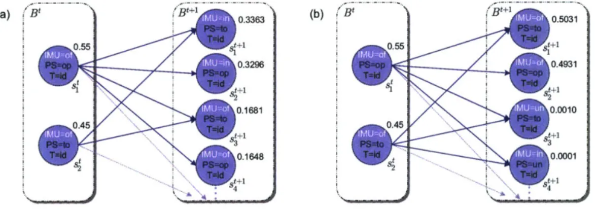
Recall the single-step belief state update example for the IMU system shown in Figure

3-2 and represented more compactly in Figure 3-3a. By framing PCCA estimation as an

OCSP and computing the belief state using Algorithm 3.1, the resulting belief state Bt+1

is shown in Figure 3-3b. The only difference is that the leading two estimates of Bt+1

in Figure 3-3a were correctly determined by Algorithm 3.1 to be inconsistent and were

not returned as valid solutions; elevating

s3+1

to st+1 in Figure 3-3b. The difference in

estimate probabilities is due to normalization over only the states that are consistent

4

.

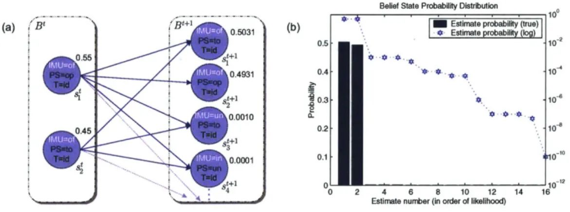
con id rigao- -i (b) . .55t+1 0 5t+1 0.3296 0.4931 0.1681 0.0010 0.45 045 t 0.1648 0.0001

Figure 3-3: Single-step belief state update example for the IMU Plant (a) solved without

considering constraints and (b) solved as an OCSP that considers constraints.

The next chapter begins by identifying 3 approximations that have previously made

online estimation tractable when scaled up to full-sized systems. The two main

contri-butions of this thesis are then presented as improvements to existing mode estimation

4_{Although framing PCCA estimation as an OCSP correctly eliminates the inconsistent states, it} introduces an error in the outgoing state transition probability distribution, such that the sum of prob-abilities across the outgoing state transitions is no longer 1. For example, since the transitions from sj to s1+1 and s2+1 in Figure 3-3a no longer exist as a solution to the OCSP, the sum of the outgoing state transition probabilities from st is 1-(0.4995)(0.1)(0.9999) -- (0.4995)(0.8995)(0.9999) = 0.5008 # 1. This is because our assumption of independent transitions is occasionally violated due to the interconnected nature of the components. One solution to this problem is to normalize the outgoing state transitions during the estimation process but this approach is not reflected in Algorithm 3.1.

38 ESTIMATION OF PCCA

approaches that, together, eliminate 2 of the 3 approximations. These two novel es-timation techniques, known as Best-First Belief State Enumeration (BFBSE)[16] and

Best-First Belief State Update (BFBSU), provide a highly accurate mode estimation

Approximate Estimation of PCCA

As space exploration systems grow increasingly complex, there is an unprecedented de-mand for accurate and reactive monitoring and diagnosis techniques that must be scalable to mounting challenges. Due to limited computational resources of embedded systems, the exact solution presented in Chapter 3 is not tractable for full-sized systems. This chapter begins by identifying three key approximations that were previously used to achieve reactivity, while preserving estimator accuracy. Section 4.2 introduces an OCSP solver that efficiently solves the approximate estimation problem using Conflict-directed

A* [22, 18] and Sections 4.3 and 4.4 adjust the A* heuristic function to eliminate two of

the three belief state update approximations.

4.1

Belief State Update Approximations

Three significant approximations are made by previous monitoring and diagnosis engines; including Livingstone [21, 15], and previously in Titan [20]:

1. The full belief state Bt is accurately approximated by maintaining only the k most likely estimates in an approximate belief state

5

3'.

2. The probability of each state is accurately approximated by the probability of the most likely trajectory to that state.

3. The observation probabilities can be accurately reduced to 1.0 for all observations consistent with the state, and 0.0 for observations inconsistent with the state.

40

APPROXIMATE ESTIMATION OF PCCA

This thesis continues to make Approximation 1 to mitigate state space explosion, but eliminates Approximations 2 and 3. The following section present each approximation in detail.

4.1.1

Exponential Belief State Approximation

For systems modeled as PCCA, there is a finite number of estimates in the belief state, though the size of the belief state is exponential in the number of concurrently operating components. More precisely, size of the belief state for n components is Ha 1..n JID(za)I, where ID(Xa)I is the number of modes in Aa. For a full-scale spacecraft propulsion subsys-tem, such as the NewMaap model of JPL's Cassini Spacecraft propulsion subsyssubsys-tem, the size of the belief state was roughly 3.580 (80 mode variables with an average domain size of 3.5) [21]. To mitigate this belief state space explosion, previous work on Livingstone and Titan have made the assumption that the true state of the system is captured within only a few of the most likely estimates. This assumption is based on the key insight that, although the full belief state is exponential in size, the bulk of the probability density is concentrated in only a handful of the most likely estimates. This is due to the drastically decreasing likelihood of simultaneous multiple point failures [7].

Recall the single-step exact belief state update OCSP example for the IMU plant, presented earlier in Section 3.2.1, and summarized again in Figure 4-la. The resulting probability distribution across all 16 consistent states in Bt+1 is shown in Figure 4-1b, where the states are ordered in terms of likelihood. The leading 2 estimates capture 99.62% of the total belief state probability density, supporting the hypothesis that the true state of the system is likely to be contained within the leading most likely estimates. By leveraging this approximation, the estimation problem is simplified from updat-ing the full belief state B to enumeratupdat-ing the k best estimates in an approximate belief state B. In order to avoid extraneous computation, preserve reactivity of the estimation process, and enable it to be employed for the purposes of real-time control, this enu-meration is performed in best-first order. Section 4.2 reviews an efficient technique for best-first estimate enumeration, based on Conflict-directed A* [221.

Belief State Probability Distribution * -* '*.. * -.. -* *--* 0.5-0.4 10.3 0.2 0.1 00 0 2

Figure 4-1: Belief state probability distribution at B

t

+

1

_{for the simple IMU Plant scenaio.}

4.1.2

Trajectory Approximation

Although the majority of belief state probability density can be captured by only a

hand-ful of most likely estimates, it is not clear how to quickly identify which estimates, out

of the entire exponential belief state, are most likely. Previous mode estimation

ap-proaches side-step this problem by unfolding the belief state transitions into a branching

tree structure (Figure 4-2) and by enumerating estimates in order of state trajectory

probability' [21, 15, 20].

BB B B

Figure 4-2: Evolution of the belief state, represented as a trellis diagram (left), can be

decomposed into a branching tree.

Each arrow on the right side of Figure 4-2 still represents a state transition, but

1

The state trajectory probability is defined as the product of state transition probability P(sj+1 si, y) and its source state probability P(sf|o0<'t>, p<0t-l>).

(a) (b)

4 6 8 10 12 14 Estimate number (in order of likelihood)

l0 102 10 -10 0 10 16