Benchmarking Exercises for Granular Flows

(1)

HAL Id: hal-03256825

https://hal.archives-ouvertes.fr/hal-03256825

Submitted on 10 Jun 2021

HAL is a multi-disciplinary open access

archive for the deposit and dissemination of

sci-entific research documents, whether they are

pub-lished or not. The documents may come from

teaching and research institutions in France or

L’archive ouverte pluridisciplinaire HAL, est

destinée au dépôt et à la diffusion de documents

scientifiques de niveau recherche, publiés ou non,

émanant des établissements d’enseignement et de

recherche français ou étrangers, des laboratoires

Benchmarking Exercises for Granular Flows

Antoine Lucas, Anne Mangeney, François Bouchut, Marie-Odile Bristeau,

Daniel Mège

To cite this version:

Antoine Lucas, Anne Mangeney, François Bouchut, Marie-Odile Bristeau, Daniel Mège. Benchmarking

Exercises for Granular Flows. 2007. �hal-03256825�

(2)

THE 2007 INTERNATIONAL FORUM ON LANDSLIDE DISASTER MANAGEMENT

Benchmarking Exercises for Granular Flows

Antoine Lucas

Institut de Physique du Globe de Paris, UMR-CNRS 7154, Université Paris Diderot, FR

Anne Mangeney

Institut de Physique du Globe de Paris, UMR-CNRS 7154, Université Paris Diderot, FR Institute for Nonlinear Sciences, UCSD, San Diego, USA

François Bouchut

Département de Mathématiques et Applications, UMR-CNRS 8553, École Normale Supérieure, FR

Marie-Odile Bristeau

Institut National de Recherche en Informatique et Automatique, Le Chesnay, FR

Daniel Mège

Laboratoire de Planétologie et de Géodynamique, UMR-CNRS 6112, Université de Nantes,FR

Abstract:

For the International Forum on Landslide Disaster Management 2007 framework, our team performed several numerical simulations on both theoretical and natural cases of granular flows. The objective was to figure out the ability and the limits of our numerical model in terms of reproduction and prediction. Our benchmarking exercises show that for almost all the cases, the model we use is able to reproduce observations at the field scale. Calibrated friction angles are almost similar to that used in other models and the shape of the final deposits is in good agreement with observation. However, as it is tricky to compare the dynamics of natural cases, these exercises do not allow us to highlight the good ability to reproduce the behavior of natural landslides. Nevertheless, by comparing with analytical solution, we show that our model presents very low numerical dissipation due to the discretization and to the numerical scheme used. Finally, in terms of mitigation and prediction, the diﬀerent friction angles used for each cases figure out the limits of using such model as long as constitutive equations for granular media are not known.

(3)

1 Introduction

1.1 Model description

Simulation is performed using the numerical model hereafter called Shaltop 2d resulting from a long term collaboration between Département de Mathématiques et Applications (DMA), École Normale Supérieure (ENS, Paris) and Institut de Physique du Globe de Paris (IPGP) in France (Bouchut et al., 2003, Bouchut 2004, Bouchut and Westdickenberg, 2004, Mangeney et al., 2005, 2007). This model was developed after former studies performed by our group in the context of a collaboration between IPGP, ENS-DMA, and INRIA. A first model was developed based on the model developed for shallow river flows by Audusse et al. (2000) and Bristeau et al., (2001).

Mangeney et al., 2003 extended this model based on a kinetic scheme to the classical Savage-Hutter model for granular flows over sloping topography with a Coulomb-type basal friction involving either a constant friction coeﬃcient or the empirical flow rule proposed by Pouliquen, (1999). Finally, the projection of the gravity field on the reference frame linked to the topography was performed during the PhD of M. Pirulli together with the active/passive earth pressure coeﬃcient [Pirulli et al., 2007] and several basal friction law have been tested on real events (Pirulli, 2004, Pirulli and Mangeney, 2007). This model after called RASH3D _{by Pirulli et al., (2007) is used in the Benchmark exercise by Pirulli}

and Scavia (report of the 2007 forum). The main advantage of this model is the unstructured finite element mesh best suited to deal with complex topography. However, the numerical method is only of order 1 and the friction, the projection of the gravity field and the introduction of the earth pressure coeﬃcients are not compatible with the preservation of steady state and do not respect all the properties required by the numerical resolution of the equations (see Bouchut, (2004), for details about numerical

methods to solve these problems). Furthermore this kinetic model (i.e. RASH3D _{model) is based on}

the Savage-Hutter equations developed in a reference frame linked to the topography including only the curvature terms in the x and y direction. Note that the afore-mentioned problems are shared with most of the numerical models proposed in the literature.

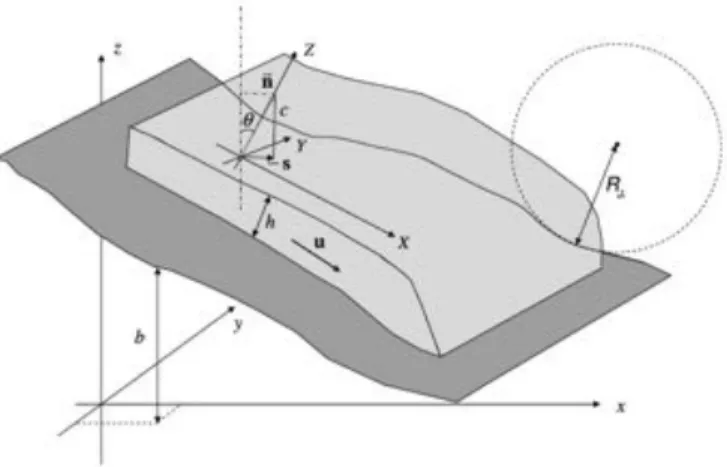
Contrary to the classical approaches, the new model Shaltop 2d is based on the equations developed by Bouchut et al., (2003) and Bouchut and Westdickenberg (2004) developed in a fixed cartesian reference frame with the thin layer approximation (TLA) imposed in the direction perpendicular to the topography (see figure 1). The rigorous asymptotic analysis makes it possible for the first time to account for the whole curvature tensor. Furthermore, the numerical method is of order 2 requiring less refined grid to reach the same precision. The numerical method is based on the work of François Bouchut (2004) and preserve the steady states as well as other requirements related to the resolution of hyperbolic equations. The overall idea is to develop the equations in a fixed reference frame (x, y, z), for example hori-zontal/vertical, as opposed to the equations developed by Hutter and co-workers in a variable reference frame linked to the topography. However, the shallowness assumptions are still imposed in the local reference frame (X, Y, Z) linked to the topography (fig. 1). Indeed, to satisfy the hydrostatic assumption for shallow flow over inclined topography, it is the acceleration normal to the topography that must be neglected compared to the gradient of the pressure normal to the topography. The reference frame is shown in figure 1. The 2D horizontal coordinate vector is x = (x, y) 2 R2_{and the topography is described}

by the scalar function b(x, y) with a 3D unit upward normal vector ~n⌘ ( s, c) 2 R2 ⇥ R, (1) where, s = rxyz p 1 + ||rxyz||2 , (2) and

(5)

Figure 1: Frames and variables used in the model (after Mangeney et al., 2007).

In the horizontal/vertical Cartesian coordinate and for a inclined plane, formulation the equations reduce to

@th + c· @x(hu) + @y(hv) = 0, (4)

@tu + cu· @xu + v· @yu + c· @x(ghc) = g sin ✓ + ˜ffx, (5)

@tv + cu· @xv + v· @yv + @y(ghc) = ˜ffy, (6)

where h is the depth-thickness of the flow, g is the vertical acceleration and u(u, v) is the depth-average velocity. The two-dimensional Saint-Venant system with topography and friction is written

8 > < > : @th + @x(hu) + @y(hv) = 0,

@t(hu) + @x(hu2+ gh2/2) + @y(huv) + hg@xb = hfx,

@t(hv) + @x(huv) + @y(hv2+ gh2/2) + hg@yb = hfy,

where b(x, y) represents the 2D topography.

Debris avalanche is treated here as a single-phase, dry granular flow with Coulomb-type behavior. The transition between a static state and flowing state is modeled by introducing a threshold allowing or not the material to flow. The friction forces f(x, y, t) = (fx, fy) (see (5) and (6)) must satisfy

||f(x, y, t)||  gµ, (7)

u(x, y, t) 6= 0 ) f(x, y, t) = gµ u(x, y, t)

||u(x, y, t)||. (8)

The friction coeﬃcient is either supposed to be constant (Coulomb friction law) or depending on the thickness h and the Froude number of the flow u/pgh(hereafter called Pouliquen flow rule):

(1) Coulomb friction law defined as follow

µ = tan , (9)

where is the constant friction angle.

(2) Pouliquen friction empirical rule (Pouliquen, 1999): µ(_{||u||, h) = tan} 1+ (tan 2 tan 1) exp

✓ _hp_gh

||u|| ◆

(6)

(1999). Basically, the friction parameter is increasing for small thickness h and high velocity u. The Coulomb type friction law applied on the averaged media has been tested by comparing depth-averaged model Shaltop 2d with discrete element simulations (Mangeney et al., 2006) on the collapse of granular column of variable aspect ratio (a = Hi/Ri, where Hi and Ri are the initial thickness and radius of

the granular column). The main result was that vertical acceleration has to be included in the model if aspect ratio a > 1 are deal with.

Shaltop 2d has been used successfully to simulate laboratory experiments of granular collapse

(Mangeney-Castelnau et al., 2005), levees-channel formation (Mangeney et al., 2007) as well as real 3D avalanches in a natural context as it has been recently shown for large Martian landslides (Lucas and Mangeney, 2007).

1.2 Computing resources

We benefit of the computing facilities from the Metacentre de Données et de Calcul Parallèle of IPGP: 1.2.1 CPU Server:

• Server Bi-Xeon 5160 3.00GHz - Mem: 3Gb

- OS: Linux Fedora 8

- Compiler: Intel Fortran 10.1

• IBM e325 server bi-cpu AMD Opteron 256 - Mem: 4Gb

- OS: Linux RedHat Entreprise 3

- Compiler: pgf95 - The Portland Group Inc. Fortran 90/95 compiler 1.2.2 Parallel Computing Cluster:

• 64 x IBM x3550 bi-cpu Intel Xeon Quad-Core E5420 (512 cores) - Mem: 512 Gb

- OS: RedHat EL release 5.1 - Compiler: Intel Fortran 10.1

Time of computation could rise up to several days on the IBM e325 depending of the grid space increment and the time of the simulation. Parallelization of the code (using MPI) has been carried out by P. Stoclet at IPGP.

1.3 Softwares used

DEM (Digital Elevation Model) processing (e.g. gridding) were performed with Surfer (Goldensoftware). Visualization and rendering have been carry out under GMT (Wessel and Smith, 1991) and MatLab.

(7)

1.4 Cases studied

As previously mentioned, Shaltop 2d is appropriate for dry granular monophasic flow such as

land-slides, rock avalanches and dry sand flows. In this context, we focused our runs on the following cases eventhought water could be present in the real landslides:

• 1.Dam Break Scenario from analytical solution • 2.Laboratory Test of dry sand flow from USGS • 3.Shum Wan landslide, HK

• 4.Fei Tsui Road landslide, HK • 5.FrankSlide, CA

(8)

2 Dam-Break Scenario

2.1 Description of the scenario

This test makes it possible to calibrate the numerical modeling with analytical solution. The scenario involves movement of mass in a wide inclined channel, triggered by sudden removal of dam (fig. 2). From the analytical solution (AS) derived by Mangeney et al., (2000), profiles of the debris flow at any given time t are: h(t) = 8 > < > : H ; x  xr 1 9g cos ✓ 2c0 x t mt 2 2 ; xr< x < xl 0 ; xl x with,

m = g(cos ✓ tan sin ✓), (11)

c0= p gH cos ✓, (12) xl= 2c0t 1 2mt2, (13) xr= c0t + 1 2mt2, (14)

where H is the initial height of debris mass, g the gravity, ✓ is the slope angle and is the angle of friction. Mass debris x = 0 h H Slope angle = θ

Friction coefficient at Channel bed = tan (δ)

x

Figure 2: Initial conditions of dam-break scenario. H is the initial height of the debris mass, ✓ is the slope angle and is the angle of friction at channel bed.

We perform test using the following settings (fig. 3): • Initial height of the mass: 10m

• Slope angle: 30o

(9)

2.2 Results

Shaltop 2d is able to predict very well the analytical solution (fig. 3).

0 100 200 300 400 500 600 700 800 900 1000 0 2 4 6 8 10 12 Distance (m) Flow height (m)

Time: 10,20 & 30 secs, δ = 25° , θ = 30° , ∆x = 1.2 AS NS

Figure 3: Evolution of the flow height for both analytical and numerical solutions respectively named

AS and NS. Using a reasonable space increment x, Shaltop 2d is able to reproduce very well the

analytical solution. 500 1000 1500 2000 0 0.2 0.4 0.6 0.8 1 x in m Fluid thickness h

Figure 4: (Top) – Comparison between RASH3D _{model with analytical solution (figure from Mangeney}

et al., 2003). (Bottom) – Using the same parameters, we compare here Shaltop 2d with analytical

(10)

On figure 4, we show that, for the same parameters, Shaltop-2d better fits the analytical solutions

than RASH3D_{model (Mangeney et al., 2003). For = 4}o_{, ✓ = 5}o_{and x = 20, Shaltop 2d reproduces}

better the runout distance predicted by the analytical solution (fig. 4). The overestimation of this runout distance in the kinetic model is related to numerical diffusion. As a result, the calibration of the kinetic model in order to fit the right runout distance would lead to friction angle almost one degree higher than the real friction angle. In the simulation of real avalanches over complex topography, numerical diffusion is expected to generate larger runout distances (i.e. larger value of the fitted friction angle) using kinetic scheme or similar schemes of order 1 than that obtained with Shaltop 2d. A series of numerical test on real topography with increasing discretization is therefore necessary if the models (i.e. the fitted friction coefficients) are to be compared on real events.

(11)

3 Dry sand behavior within a 3D channel

3.1 Description of the simulation

Simulation of the experimental results of Iverson et al. (2004) dealing with dry granular flows over irregular 3D channel (see figure 3) is performed here.

The basal topography has the following characteristics (fig. 5): • Mean angle of sloping flume bed: 31.6o

• Headgate aperture width: 12 cm • X location of headgate: 8.858 cm.

• Location of urethane topographic insert: entire flume width (20 cm), and covering from x = 9.14 cm to x = 39.12 cm.

• The right triangular prism that spans the full width of the flume (20cm) is approximately h0= 4.35 cm

thick (measured vertically) at x = 8.858 cm (headgate) and tapers to 0 cm thick upflume from the headgate at x ' 1.9 cm.

We interpolate (using kriging algorithms) the DEM so as to get a space increment x = y = 0.24 cm.

Figure 5: 3D irregular channel with the initial mass (in color).

Results obtained using a constant friction coeﬃcient all over the topography are obviously not accu-rate because substaccu-rates with diﬀerent roughness were used in the tank and in the irregular topography. Numerical simulation usign = 29 all over the numerical domain is however shown for comparison (see fig. 7). The bottom part of the mass spreading is quiet well reproduce by the code, whereas the top part does not fit with Iverson et al., 2004 observations. Mass staying in the tank is overestimated within the sand tank at the end of the simulation. As consequences, 15% of the bulk mass don’t participate in the spreading.

As mentioned in Iverson et al., 2004, two kind of materials are used in this 3D channel. The tank

and the bottom parts are made of Formica with a bed friction angle f = 23.5o and the channel part

with urethane characterized by a bed friction angle u = 19.8o. We thus adapt our code so as to take

into account the variation of the bed friction angle due to the diﬀerent floor (Formica and urethane). Results are obviously significantly improved as shown in figure 8. Mass profile is more alike experimental observations (top of fig. 6).

(12)

(13)

Figure 7: Evolution of the dry granular media across an irregular 3D channel using a single friction angle = 29o _{all over the numerical domain (DEM courtesy Iverson et al., 2004)}

(14)

(15)

Velocity Stats. Time (sec.) u (m.s 1_{) U} max(m.s 1) /u 4 2.39 11.18 2.71 1.14 16 5.16 16.53 4.85 0.94 28 2.56 13.35 4.17 1.62

Table 1: Velocity evolution and statistics for Shum Wan landslide

4 Shum Wan landslide, HK (1995)

4.1 Description of the simulation

Analysis of Fei Tsui landslide has been carried out using Coulomb-type friction law. The initial volume in our simulation is 26.103 _m3_{. Using griding algorithms (e.g. kriging) we get a 2 m grid spacing. The grid}

is 113 x 85 points. We performe several analysis dealing with Coulomb-type friction angle 2 [16o_{, 26}o_].

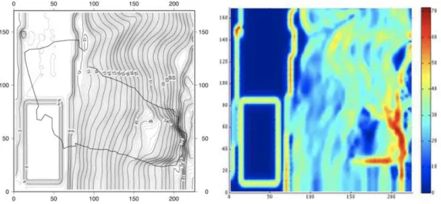
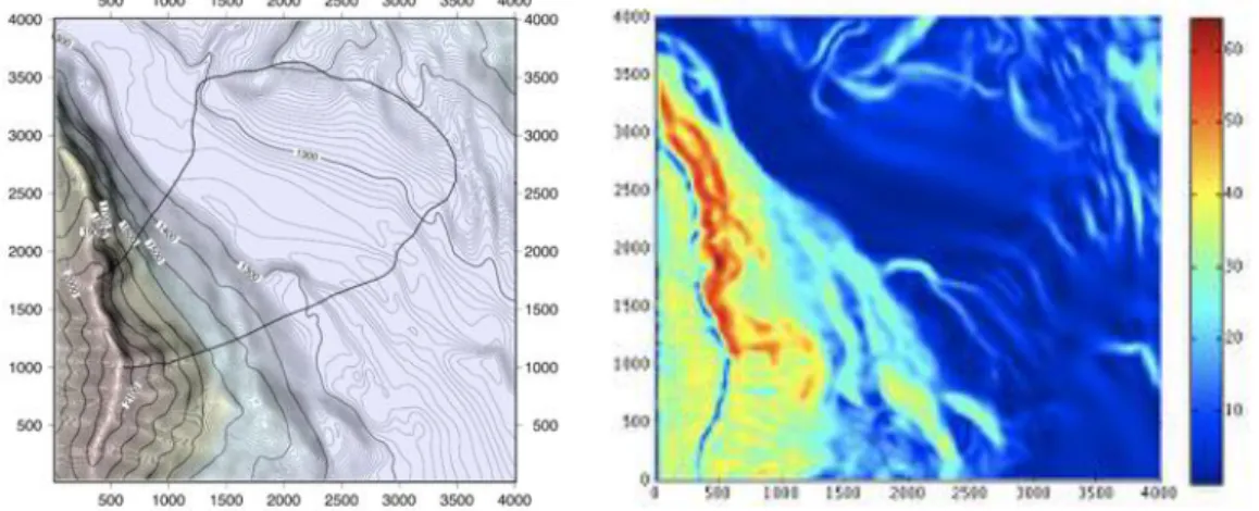
Figure 9: (Left) – DEM of Shum Wan landslide, HK. Slide path is indicated by black lines over the topographic map. (Right) – Slope map calculated from the DEM.

4.2 Results

The friction angle is calibrated to fit the runout distance of the landslide. Best agreement is obtained using = 18o_{. The mean velocity increases with a factor two during the 10 first seconds. The flow stops}

(16)

(17)

Velocity Stats. Time (sec.) u (m.s 1_{) U} max(m.s 1) /u 2 4.5 29.05 3.40 0.76 8 2.38 68.33 3.08 1.29 14 1.34 47.39 2.35 1.75

Table 2: Velocity evolution and statistics for Fei Tsui landslide

5 Fei Tsui landslide, HK (1995)

5.1 Description of the simulation

Analysis of Fei Tsui landslide has been carried out using Coulomb-type friction and Pouliquen friction laws. The initial volume in our simulation is 14.103 _m3 _{with a 1m grid spacing. The grid is 97x117}

points. A series of simulation is performed using friction angles 2 [22o_{, 30}o_].

Figure 11: (Left) – DEM of Fei Tsui landslide, HK. Slide path is indicated by black lines over the topographic map. (Right) – Slope map from the DEM.

5.2 Results

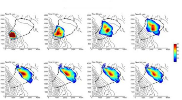
Better results are obtained with = 26o _{as it is shown on Figure 12. On the right side of Figure 12,}

we show the evolution of the velocity field at several times. The mean velocity increases rapidly after triggering and rise up to 70 m/s at its maximum. The flow stops at t ' 15 s ( (see table 2).

Finest analysis shows that between t = 8 s and t = 14 s, the back of the mass is still under movement whereas the front does not.

As consequences, the flow spread on each side (along the road) and not in the slope direction. We thus overestimate the width of the final deposits.

(18)

10 20 30 40 50 60 70 80 90 100 110 10 20 30 40 50 60 70 80 90 10 m/sec 3 3 3 3 6 6 6 9 9 10 20 30 40 50 60 70 80 90 100 110 10 20 30 40 50 60 70 80 90 Times: 2 secs 10 20 30 40 50 60 70 80 90 100 110 10 20 30 40 50 60 70 80 90 10 m/sec 3 3 3 3 3 6 6 6 10 20 30 40 50 60 70 80 90 100 110 10 20 30 40 50 60 70 80 90 Times: 8 secs 10 20 30 40 50 60 70 80 90 100 110 10 20 30 40 50 60 70 80 90 10 m/sec 3 3 3 3 3 6 6 9 10 20 30 40 50 60 70 80 90 100 110 10 20 30 40 50 60 70 80 90 Times: 14 secs

(19)

6 Frank Slide, CA (1902)

6.1 Description of the simulation

The frank slide involves 36.106 _m3_{. The grid is 201 x 201 points with 20 m space increment.}

Figure 13: (Left) – DEM of Frank Slide, CA. Slide path is indicated by black lines over the topographic map. (Right) – Slope map calculated from the DEM.

6.2 Results

Pirulli and Mangeney (2007) proposed a Coulomb-type friction angle = 14o_{for this specific landslide.}

Using the same angle Shaltop 2d underestimates the observed runout as it is shown on figure 14.

We get better results with = 12o _{(fig. 15). Using a Pouliquen-type friction law, we get very similar}

results (fig. 16). Sensitivity of the numerical results to mesh size has to be performed before getting any conclusion from this comparison. Actually, the diﬀerences could only result from numerical dissipation (see discussion in the analytical solution section).

(20)

(21)

(22)

Velocity Stats. (Coulomb-type Friction) Time (sec.) u (m.s 1_{) U} max (m.s 1) /u 10 7.25 15.31 3.71 0.51 40 20.26 67.00 13.54 0.67 70 3.85 69.80 8.85 2.30

Velocity Stats. (Pouliquen-type Friction)

Time (sec.) u (m.s 1_{) U}

max (m.s 1) /u

10 7.30 15.16 3.81 0.55

40 20.80 76.14 13.50 0.65

70 3.97 47.25 8.65 2.17

Table 3: Velocity evolution and statistics for both behaviors.

Using Coulomb-type friction or Pouliquen-type friction law has consequences on velocity field. With the second law, the flow gets faster but slows down quickly compare to Coulomb-type friction law (see table 3).

(23)

7 Conclusion

Our simulations shows that despite the accordingly nonphysical empirical friction coeﬃcient used in the numerical model, the area of the deposit is quite well reproduced in many natural cases. However, we showed that this coeﬃcient ranges between 12o _{and 28}o_{depending on the studied case. This dispersion}

of the friction coefficient questions the predictable power of this approach. The presence of a fluid phase, granulometry distribution, the presence of tree roots at the top of the released mass as this is the case for Shum Wan slide or Fei Tsui slide could explain the difference between the friction coefficient. Only calibration in the similar geological context would possibly make it possible to predict further events.

Using both friction laws (Coulomb and Pouliquen) may have inferences on velocity field. In terms of prediction, this is a key point, because of the pressure impact on the foundations.

(24)

References

Audusse, E., Bouchut, F., Bristeau, M.-O., Klein, R., Perthame, B., A fast and stable well-balanced scheme with hydrostatic reconstruction for shallow water flows, SIAM J. Sci. Comp. 25, 2050-2065, 2004

Bouchut, F. Nonlinear stability of finite volume methods for hyperbolic conservation laws, and well-balanced schemes for sources, Frontiers in Mathematics series, Birkh¨auser, 2004

Bouchut, F, Mangeney-Castelnau, A., Perthame, B., Vilotte, J.-P., A new model of Saint Venant and Savage-Hutter type for gravity driven shallow water flows, C.R. Acad. Sci. Paris, série I 336, 531-536, 2003

Bouchut, F. and Westdickenberg, M., Gravity driven shallow water models for arbitrary to-pography, Comm. in Math. Sci. 2, 359-389, 2004

Bristeau, M.-O., Coussin, B., Perthame, B., Boundary conditions for the shallow water equa-tions solved by kinetic schemes, INRIA Report, 4282, 2001

Iverson, R. M., Logan, M., and Denlinger, R.P., Granular avalanches across irregular three-dimensional terrain: 2. Experimental tests, J. Geophys. Res., 109, F01015, 2004

Lucas, A. and Mangeney, A., Mobility and topographic eﬀects for large Valles Marineris landslides on Mars, Geophys. Res. Lett., 34, L10201, doi:10.1029/2007GL029835, 2007.

Mangeney-Castelnau, A., Vilotte, J.-P., Bristeau, M.-O., Perthame, B., Bouchut, F., Simeoni, C., Yernini, S., Numerical modeling of avalanches based on Saint-Venant equations using a ki-netic scheme, J. Geophys. Res.108 (B11), 2527, 2003

Mangeney-Castelnau, A., Bouchut F., , Vilotte, J.-P., Lajeunesse, E., Aubertin, A., Pirulli, M., On the use of Saint-Venant equations for simulating the spreading of a granular mass, J. of Geophysical Research, 110(B9):B09103, 2005

Mangeney, A., Staron, L., Volfson, D., and Tsimring, L., Comparison Between Discrete and Continuum Modeling of Granular Spreading, WSEAS Transactions on Mathematics, 2(6), pp. 373-380. 2006

Mangeney, A., Bouchut, F., Thomas, N., Vilotte, J.-P., Bristeau, M.-O., Numerical modeling of self-channeling granular flows and of their levee/channel deposits, J. Geophys. Res. Earth Surface, 112, F02017, 2007

Pirulli, M., Numerical modelling of landslide runout, a continuum mechanics approach. PhD. The-sis in Geotechnical Engineering, Supervisor: Claudio Scavia, Politecnico di Torino, Anne Mangeney, IPGP-Université Paris-Diderot, France, Oldrich Hungr, University British Columbia, Vancouver. 2004

Pirulli, M., Bristeau, M.-O., Mangeney, A., and Scavia, C., The eﬀect of the earth pressure coef-ficients on the runout of granular material, Environmental Modelling and Software, 22, 1437-1454, 2007

(25)

Wessel, P. and Smith, W. H. F., Free software helps map and display data, EOS Trans. AGU, 72, 441, 1991