HAL Id: hal-02570584
https://hal.sorbonne-universite.fr/hal-02570584
Preprint submitted on 12 May 2020
HAL is a multi-disciplinary open access
archive for the deposit and dissemination of
sci-L’archive ouverte pluridisciplinaire HAL, est destinée au dépôt et à la diffusion de documents
Automatic analysis of insurance reports through deep
neural networks to identify severe claims
Isaac Cohen Sabban, Olivier Lopez, Yann Mercuzot
To cite this version:
Isaac Cohen Sabban, Olivier Lopez, Yann Mercuzot. Automatic analysis of insurance reports through deep neural networks to identify severe claims. 2020. �hal-02570584�
Automatic analysis of insurance reports
through deep neural networks to identify
severe claims.
Isaac Cohen Sabban
∗1,2Olivier Lopez
∗1, Yann Mercuzot
2.
May 12, 2020
Abstract
In this paper, we develop a methodology to automatically classify claims using the information contained in text reports (redacted at their opening). From this automatic analysis, the aim is to predict if a claim is expected to be particularly severe or not. The difficulty is the rarity of such extreme claims in the database, and hence the difficulty, for classical prediction techniques like logistic regression to accurately predict the outcome. Since data is unbalanced (too few observations are associated with a positive label), we propose different rebalance algorithm to deal with this issue. We discuss the use of different embedding methodologies used to process text data, and the role of the architectures of the networks.
Key words: Insurance; Deep neural networks; Long Short Term Memory; Convolutional Neural Networks; Text analysis.
Short title: Insurance reports through deep neural networks
1Sorbonne Universit´e, CNRS, Laboratoire de Probabilit´es, Statistique et Mod´elisation,
LPSM, 4 place Jussieu, F-75005 Paris, France
2Pacifica, Cr´edit Agricole Assurances, F-75015 Paris, France
1
Introduction
The automatization of text data analysis in insurance is a promising and challenging field, due to the importance of reports and analysis in the treatment of claims or contracts. In this paper, we focus on data coming from expert reports on a claim, but textual informations may be found also in declarations filled by policyholders themselves, or in medical questionaries used in credit insurance. Our aim is to process these reports and develop an automatic way to categorize the corresponding claims and to identify, soon after their occurrence, which one will lead to a heavy loss. Apart from the complexity of the input information, a particular difficulty is caused by the rareness of such claims (a few percent of the total database).
The rise of deep learning techniques introduces the possibility of developing an au-tomated treatment of these data, with potential reduced costs - and, ideally, a more accurate analysis - for the insurance company, hence a potential increase of rentability. Text mining has received a lot of attention in the past decades in the machine learning literature, with many spectacular examples. Many examples can be found, for example, in [1] or [6], with applications to insurance such as [14] or [24].
As we already mentioned, our main difficulty is to focus on the prediction of relatively rare events, which is a classical specificity of the insurance business compared to other fields. Indeed, while typical claims and behavior are usually easy to understand and measure, the tail of the distribution of the losses is much more delicate, since there are quite few events in the database to evaluate it properly. Of course, these so-called ”extreme” events may, in some cases, constitute an important part of the total losses at a portfolio level.
In this paper, we consider the case of text data coming from experts in view of cluster-ing some claims dependcluster-ing on their severity. Typically, the insurance company wants to separate ”benign” claims from the heaviest ones in order to perform a different treatment of these two types of claims. Indeed, in terms of reserving, a different model can be used on these two types of events. Moreover, a particular attention can then be devoted to the most serious claims during their development. As described above, the difficulty is that the proportion of heavy claims is quite low compared to the other class. This imbalance is present in other potential applications, such as fraud detection. We rely on deep neural networks methodologies. Neural networks have already demonstrated to be valuable tools when it comes to evaluating claims, see for example [37] or [41]. The network
architec-tures that we use - convolutional neural networks, see [4], and recurrent neural networks (such as Long Short Term Memory networks introduced by [18]) - are powerful tools to perform such text analysis, see for example [29] and [11]. The specificity of our approach is twofold:
• we introduce a bias correction in order to deal with the fact that claim development time may be long: indeed, our models are calibrated on a database made of claims that are closed, but also from unsettled ones. Calibrating the model on the closed claims solely would introduce some bias due to the over-representation of claims with small development time (this is a classical problem linked to the concept of censoring in survival analysis, see e.g. [27],[16]).
• once this bias correction has been done, a re-equilibration of the database is required to compensate the rareness of the events we focus on. For this, we use Bagging methodologies (for Bootstrap Aggregating, see [9]), introducing constraints in the resampling methodology which is at the core of Bagging.
The rest of the paper is organized as follows. In section 2 we describe the general framework and the general methodology to address these two points. A particular focus on processing text data is shown in section 3, where we explain the process of embedding such data (this means to perform an adapted dimension reduction to represent efficiently such complex unstructured data). The deep neural networks architectures that we use are then described in section 4. In section 5, a real example on a database coming from a French insurer gives indications on the performance of the methodology.
2
Framework and neural network predictors
In this section, we describe the generic structure of our data. Our data are subject to random censoring, as a time variable (time of settlements of the claims) is present in the database. The correction of this phenomenon, via classical methodologies from survival analysis, is described in section 2.1. Next the general framework of neural networks is defined in section 2.2. The imbalance in the data, caused by the fact that we focus on predicting rare events, is described in section 2.3, along with methodologies to improve the performance of our machine learning approaches under this constraint.
2.1
The censoring framework
Our aim is to predict a 0-1 random response I, which depends on a time variable T and covariates X ∈ X ⊂ Rd. In our practical application, I is an indicator of the severity
of a claim (I = 1 if the claim is considered as ”extreme”, 0 otherwise). The definition of what we refer to as an extreme claim depends on management conventions that will be described in the real data section. The variable T represents the total length of the claim (i.e. the time between the claim occurence and its final settlement), and X some characteristics.
In our setting, the variables I and T are not observed directly. Since T is a duration variable, it is subject to right-censoring. This means that, for the claims that are still not settled, T is unknown. On the other hand, I is known only if the claim is closed. This leads to the following observations (Ji, Yi, δi, Xi)1≤i≤n assumed to be i.i.d. replications of
(J, Y, δ, X) where Y = inf(T, C), δ = 1T ≤C, J = δI,
and X represents some covariates that are fully observed (in our case, X is text data com-ing from reports, hence it can be understood as a vector in Rd with d being huge: more precisely, X can be understood as a matrix, each column representing an appropriate cod-ing of a word, see section 3, the number of columns becod-ing the total number of words). The variable C is called the censoring variable and is assumed to be random. The censoring variable corresponds to the time after which the claim stops to be observed for any other reason than its settlement (either because the observation period ends before settlement, or because there has been a retrocession of the claim). This setting is similar to the one developed by [28] or [27] in the case of claim reserving, with a variable I that may not be binary in the general case. In the following, we assume that T and C have continuous distributions so that these variables are perfectly symmetric (otherwise, a dissymmetry can appear due to ties).
Considering only the complete data (i.e. with δi = 1, which corresponds to the case
where the claim is settled) would introduce some bias: among the complete of observa-tions, there is an overrepresentation of claims associated with a small value of Ti. Since
T and I are dependent (in practice, one often observes a positive correlation between T and the corresponding amount of the claim), neglecting censoring would imbalance the
Our aim is to estimate the function π(x) = P(I = 1|X = x), in a context where the dimension d of x is large. Typically, how an estimated function fits data is quantified by minimizing some loss function. If we were dealing with complete data, a natural choice would be the logistic loss function (also called ”cross entropy” in the neural network literature, see for example [23]), that is
L∗n(p) = −1 n n X i=1 {Iilog p + (1 − Ii) log(1 − p)} ,
which is a consistent estimator of
L(p) = −E [I log p + (1 − I) log(1 − p)] .
As stated before, computation of L∗n is impossible in presence of censoring due to the lack of information, and an adaptation is required to determine a consistent estimator of L.
A simple way to correct the bias caused by censoring is to rely on the Inverse Prob-ability of Censoring Weighting (IPCW) strategy, see for example [35]. The idea of this approach is to find a function y → W (y) such that, for all positive function ψ with finite expectation,
E [δW (Y )ψ(J, Y, X)] = E [ψ(I, T, X)] , (2.1) and to try to estimate this function W (in full generality, this function can also depend on X). The function W depends on the identifiability assumptions that are required to be able to retrieve the distribution of I and T from the data. In the following, we assume that
1 C is independent from (J, T ) 2 P(T ≤ C|I, T, X) = P(T ≤ C|T ),
as in [27], and is similar to the one used, for example, in [39] or [40] in a censored regression framework. These two conditions ensure that (2.1) holds to W (y) = SC(y)−1 = P(C ≥
y)−1. SC can then be consistently estimated by the Kaplan-Meier estimator (see [21]),
that is ˆ SC(t) = Y Yi≤t 1 − Pn δi j=11Yj≥Yi . !
Consistency of Kaplan-Meier estimator has been derived by [38] and [3]. Hence, each quantity of the type E [ψ(I, T, X)] can be estimated byPn
i=1Wi,nψ(Ji, Yi, Xi),
where
In other words, a way to correct the bias caused by the censoring consists in attributing the weight Wi,n at observation i. This weight is 0 for censored observations, and the missing
mass is attributed to complete observations with an appropriate rule. A convenient way to apply this weight once and for all is to duplicate the complete observations in the original data accordingly to their weight. This is a way to artificially (but consistently) compensate the lack of complete observations associated with a large value of Yi (let us
observe that Wi,n is an increasing function of Yi). This leads to the following duplication
algorithm.
Algorithm 1 Duplication algorithm for censored observations Require:
- a dataset (Ji, Yi, δi, Xi)1≤i≤n.
- a list of weights Wi,n computed from the data accordingly to (2.2), and let w =
min1≤i≤nWi,n.
Set n0 = 1.
for i ← 1 to n do
1. If δi = 0, go to step i + 1.
2. Else:
• Let k = bWi,n/wc , where bxc denotes the integer part of x.
• Define, for j ∈ {1, ..., k} Jn00−1+j = Ji, Yn00−1+j = Yi, Xn0−1+i = Xi.
• n0 ← n0+ k.
end for
return The duplicated dataset: (Zi)1≤i≤n0 = (Ji0, Yi0, X0i)1≤i≤n0.
The cross-entropy that we want to minimize is then computed from the duplicated dataset, defining Ln0(p) = − 1 n0 n0 X i=1 {Ji0log p + (1 − Ji0) log(1 − p)} . (2.3)
loss functions, which can be seen as modifications of cross-entropy. The focal-loss (see [26]) is defined as ˜ Ln0(p) = − 1 n0 n0 X i=1 {Ji0γlog p + (1 − Ji0)γlog(1 − p)} . (2.4) where γ ≥ 0. The parameter γ helps to focus on ”hard” examples, by avoiding attributing too much weights at easily well-predicted observations. The Weighted Cross Entropy (see [30]) is a weighted version of (2.3). Introducing a weight α ∈ (0, 1), define
¯ Ln0(p) = − 1 n0 n0 X i=1 {Ji0α log p + (1 − α)(1 − Ji0) log(1 − p)} . (2.5) The parameter α can be used to increase the importance of good prediction for one of the two classes, or to reflect its under-representation in the sample.
2.2
Neural network under censoring
A neural network (see for example [17], chapter 11) is an over-parametrized function x → p(x, θ), that we will use in the following to estimate function π. By over-parametrized, we mean that θ ∈ Rk, with k usually much larger than d (the dimension of x). The
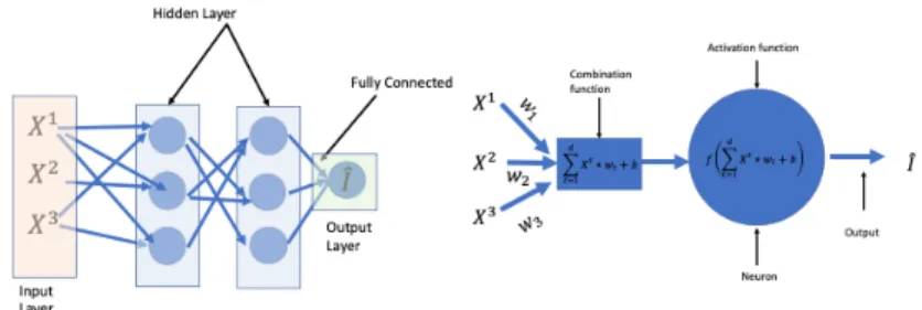
function p(·, θ) can also have a complex structure depending on the architecture of the network, that we present in more details in section 4. Typically, a neural network is a function that can be represented as in Figure 1. Following the notations of Figure 1, each neuron is described by a vector of weights w (of the same size as x), a bias term b (1-dimensional), and an activation function f used to introduce some nonlinearity. Typical choices of functions f are described in Table 7. Following our notations, θ represents the list of the weights and bias parameters corresponding to all neurons of the network. For a given value of θ and an input x, the computation of p(x, θ) is usually called ”forward propagation”.
On the other hand, ”backward propagation” (see [36]) is the algorithmic procedure used to optimize the value of the parameter θ. Since our aim is to estimate the function π, fitting the neural network consists of trying to determine
θ∗ = arg min
θ Ln
0(p(·, θ)),
where we recall that Ln has been defined in equation (2.3) (or, alternatively, using ˜Ln0 or
¯
Ln0 from (2.4) and (2.5)), and is adapted to the presence of censoring since computed on
Figure 1: Left-hand side: representation of a simple neural network (multilayer percep-tron). Each unit of the network (represented by a circle), is called a neuron (a neuron is represented on the right-hand side). X(j)represents the j−th component of the covariate vector X.
2.3
Bagging for imbalanced data
Bagging (for bootstrap aggregating, see [9]) is a classical way to stabilize machine learning algorithms. Bootstrap resampling is used to create pseudo-samples. In our case, a differ-ent neural network is fitted from each pseudo-sample, before aggregating all the results. Introducing bootstrap is expected to reduce the variance of estimation, while avoiding overfitting.
Algorithm 2 Bagging algorithm applied to neural networks Require:
- a neural network architecture, that is a function θ → p(·, θ);
- a subset of the original data (Zi0)1≤i≤m= (Zσ(i))1≤i≤m for m ≤ n and σ a permutation
of {1, ..., n};
- B the number of iterations of the algorithm (number of estimators that are aggre-gated).
for k ← 1 to B do
1. Draw a bootstrap sample (Zi(k)) from (Zi0)1≤i≤m.
2. Fit p(·, ˆθ(k)) on this bootstrap sample. end for
return The final estimator is x → ˆπ(x) = B1 PB
k=1p(x, ˆθ(k)).
A particular difficulty in applying bagging to our classification problem is that we have a problem in which a class is under-represented among our observations. If we were to apply bagging as in Algorithm 2 directly, many bootstrap samples may contain too few observations from the smallest class to produce an accurate prediction. This could limit considerably the performance of the resulting estimator.
For structured data, methods like SMOTE (see [10]) can be used to generate new observations to enrich the database. Data augmentation techniques are also available for image analysis, see [34]. These techniques are difficult to adapt to our text analy-sis framework, since they implicitly rely on the assumption that there is some spatial structure underlying data: typically, if the observations are represented as points in a multi-dimensional space, SMOTE joins two points associated with label 1, and introduce a new pseudo-observation somewhere on a segment joining them. In our situation, la-bels are scattered through this high-dimensional space, and the procedure does not seem adapted.
We here propose two simple ways to perform rebalancing, that we refer to as ”Balanced bagging” and ”Randomly balanced bagging” respectively.
Algorithm 3 Balanced Bagging Algorithm Require:
- same requirements as in Algorithm 2.
- n1 = number of desired observations in the under-represented class (corresponding
to Ji0 = 1, denoted C1).
for k ← 1 to B do
1. Draw a bootstrap sample (Zi(k))1≤i≤2n1 from (Z
0
i)1≤i≤m, under the constraint
that (Zi(k))1≤i≤n1 ∈ C1 and (Z
(k)
i )n1+1≤i≤2n1 ∈ C0 (where C0 denotes the class of
observations such that Ji0 = 0).
2. Fit p(·, ˆθ(k)) on this bootstrap sample.
3. Compute the corresponding fitting error ek, and let wk = e−1k .
end for
return The final estimator is x → ˆπ(x) = PB1 j=1wj
PB
k=1wkp(x, ˆθ (k)).
Algorithm 4 Randomly Balanced Bagging Algorithm Require:
- same requirements as in Algorithm 2.
- n1 = mean number of desired observations in the under-represented class.
- a such that n1+ a is less than the total number of observations in C1.
for k ← 1 to B do
1. Simulate two independent variables (U0, U1) uniformly distributed on [−a, a],
and define ˆn0 = n1+ U0, ˆn1 = n1+ U1.
2. Draw a bootstrap sample (Zi(k))1≤i≤ˆn0+ˆn1 from (Z
0
i)1≤i≤m, under the constraint
that (Zi(k))1≤i≤ˆn1 ∈ C1 and (Z
(k)
i )ˆn1+1≤i≤ˆn1+ˆn0 ∈ C0.
3. Fit p(·, ˆθ(k)) on this bootstrap sample.
4. Compute the corresponding fitting error ek, and let wk = e−1k .
end for
return The final estimator is x → ˆπ(x) = PB1 j=1wj
PB
k=1wkp(x, ˆθ (k)).
In each case, the final aggregated estimator perform the synthesis of each step, giving more importance to step k if its fitting error ek is small.
2.4
Summary of our methodology
Let us summarize our methodology, which combines bias correction (censoring correction), and bagging strategies to compute our predictor. First, we compute Kaplan-Meier weights and use them to duplicate data according to these weights as described in Algorithm 1. Then, from a given neural network architecture, we use one of the bagging algorithm of section 2.3 to create pseudo-samples, and aggregate the fitted networks to obtain our final estimator ˆπ(x).
The quality of the prediction strongly depends on two aspects that have still not been mentioned in this general description of the method:
• Pre-processing of text data: this step consists in finding the proper representa-tion of the words contained in the reports in a continuous space, adapted to defining
a proper distance between words.
• Architecture: the performance is strongly dependent on the type of neural net-works used (number of layers, structure of the cells and connexions).
This two points are developed in section 3 and 4 respectively.
3
Embedding methodology
In this section, we discuss the particularity of dealing with text data. To be analyzed by neural networks structures, text data first require to be transformed into covariates of large dimension in an appropriate space. After discussing one-hot encoding in section 3.1, we will explain the concept of word embedding in section 3.2. A combination of the standard Fasttext embedding methodology (see [19]) with our database of text reports is discussed in section 3.2.1.
3.1
One-hot encoding
Since our procedure aims at automatically treating text data and use them to predict the severity of a claim, we need to find a convenient representation of texts so that it can be treated efficiently by our network. A first idea is to rely on one-hot encoding. The set of whole words in the reports forms a dictionary of size V (Vocabulary size), then each word is associated to a number 1 ≤ j ≤ V. A report is then represented as a matrix. If there is l words in the report, we encode it as a matrix X = (xa,b)1≤a≤V,1≤b≤l, with V lines and l
columns. The k−th column represents the k−th word of the report, say xk. If this word
is the j−th word of the dictionary, then xj,k = 1 and xi,k = 0 for all i 6= j. Hence, each
column has exactly one non-zero value.
To introduce some context of use of the words, the size of the dictionary can be in-creased by not considering single words but n−grams. A n-gram is a contiguous sequence of n items from a given sample of text or speech (either a sequence of words, or of letters). The vocabulary size V becomes the total number of n−grams contained in the report.
Using one-hot encoding makes the data ready for machine learning treatment, but it raises at least two difficulties:
- it is not adapted to defining a convenient distance between words. Indeed, we want to take into account that there are similarities between words (synonyms, for instance, or even spelling errors).
Hence, there is a need for a more compact representation that would define a proper metric on words.
3.2
Word embedding
This process of compacting the information is called word embedding, see [7], [20]. The idea of embedding is to map each column of a one-hot encoded matrix to a lower dimension vector (whose components are real numbers, not only 0-1 valued).
Embedding consists in defining dense vector representations of the characters. The objectives of these projections are:
- Dimension Reduction: as already mentioned, embedding maps a sparse vector of size V to a lower dense vector of size N < V .
- Semantic Similarity: typically, words that are similar or that are often associated, will be close in terms of embedded vectors.
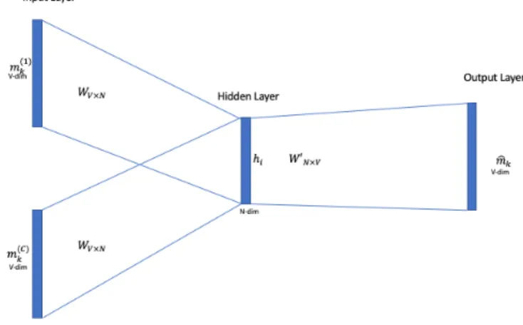
To perform embedding, we will use a linear transform of vectors. This transformation is defined by the embedding matrix W (V columns and N lines). A one-hot encoded report X is then transformed into X0 = W X (according to the notations of section 2), which becomes the input of our neural network models. How to determine a proper matrix W is described by the diagram of Figure 2. A full description of the steps of the methodology is the following:
• a ”context window” of size c = 2p + 1 is centered on the current word xk: this
defines a set of c words (xk−j)−p≤j≤p that are used as inputs of the procedure of
Figure 2.
• the embedding matrix W is applied to each of these word, and an hidden layer, producing, for the k−th group of words, hk= C−1
Pp
j=−pW xk.
• the N −dimensional vector hk is then sent back to the original V −dimensional space
by computing ˆxk = W0hk = (ˆxj,k)1≤j≤V, where W0 denotes the synaptic matrix of
The error used to measure the quality of the embedding for word k is − V X j=1 log exp(xj,kxˆj,k) PV l=1exp(xl,kxˆl,k) ! .
A global error is then obtained by summing all the words of the report, and by summing over all the reports. The embedding matrix is the one which minimizes this criterion.
Figure 2: Summary of the embedding matrix determination.
3.2.1 FastText
The gist of FastText, see [19], is that instead of directly learning a vector representation for a word (as with word2vec, see [33]), the words are decomposed into small character n-grams (see [8]), and one learns a representation for each n-gram. A word is represented as words being represented as the sum of these representations. So even if a word is misspelled, its representation tends to be close to the one of the well-spelled word. More-over, FastText proposes an efficient algorithm to optimize the choice of the embedding matrix. A pre-trained FastText embedding matrix is available, trained on a huge number of words. Nevertheless, it has not been calibrated from on a vocabulary and a context specific to insurance. Hence, a possibility that we develop in the following is to use the FastText algorithm (not the pre-trained matrix), but training our embedding matrix on the corpus of insurance reports from our database.
In the following, we distinguish between three ways of performing embedding:
be-architectures described in the following section 4. Only the parameters of these networks are iteratively optimized. We call this method ”static” embedding. • the embedding is considered as a first (linear) layer of the network. The values of
the embedding matrix W are initialized with FastText’s algorithm, but updated at the same time the other coefficients of the network are optimized. We call this method ”non-static”.
• for comparison, we also consider the case of a random initialization of this matrix W, whose coefficients are then updated in the same way as in the non-static method. We refer to it as the ”random” method.
4
Network architectures for text data
The architecture of neural networks is a key element that can considerably impact their performance. We consider to types of architectures in the following:
• Convolutional Neural Networks (CNN), described in section 4.1;
• Long Short Term Memory (LSTM) networks which are a particular kind of Recur-rent Neural Networks (RNN), described in section 4.2.
4.1
Convolutional Neural Network
Convolutional Neural Networks are nowadays widely used for image processing (image clustering, segmentation, object detection...), see for example [25]. [22] showed that they can achieve nice performance on text analysis. Compared to the multilayer perceptron, which is the most simple class of neural network and corresponds to the architecture described in Figure 1, CNN are based on a particular spatial structure that prevents overfitting.
A CNN is made of different type of layers composing the network. One may distinguish between:
• convolutional layers: each neuron only focus on a localized part of the input, see below;
• fully connected layers: every neuron of the layer is connected to every neuron in the following one;
• normalization layers: used to normalize the inputs coming from the previous layer; • padding and pooling layers: the aim is either to expand or to reduce the dimension of the inputs coming from the previous layer through simple operations, see below; • the final output layer that produces a prediction of the label through combination
of the results of the previous layer.
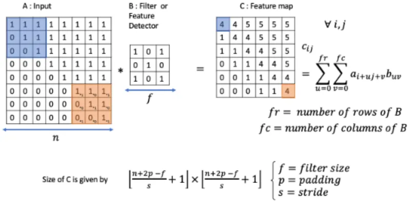
The convolutional layers are at the core of the idea of spatial structure of CNNs. They extract features from the input while preserving the spatial relationship between the coordinates of the embedding matrix. Typically, they operate simple combinations of coefficients whose coordinates are closed to each other, as illustrated in Figure 3.
Figure 3: An example of a convolution layer. Convolution Layer. Each coefficient ci,j
of the output matrix is obtained by a linear combinations of coefficients ai,j in a f × f
square of the input matrix. The color code shows which coefficients of the input matrix have been used to compute the corresponding coefficient of C.
In CNN terminology, the matrix B in Figure 3 is called a ‘filter‘ (sometimes ’kernel’ or ’feature detector’) and the matrix formed by sliding the filter over the input and computing the dot product is called the ‘Convolved Feature’ (‘Activation Map’ or ‘Feature Map‘). A filter slides over the input (denoted by A in Figure 3) to produce a feature map. Each coefficient of the output matrix (C in Figure 3) is made of a linear combination of the coefficients of A is a small square of the input matrix. This linear combination is a convolution operation. Each convolution layer aims to capture local dependencies in the original input. Moreover, different filters make appear different features, that is different structures in the input data. In practice, a CNN learns the values of these filters on its
number of filters, filter size, architecture of the network etc. before the training process). The higher the number of filters, the more features get extracted, increasing the ability of the network to recognize patterns in unseen inputs.
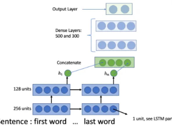
The other types of layers are described in section 7.2. An example of CNN architecture is described in the real data application, see Figure 7.
4.2
Recurrent Neural Networks and Long Short Term Memory
(LSTM) networks
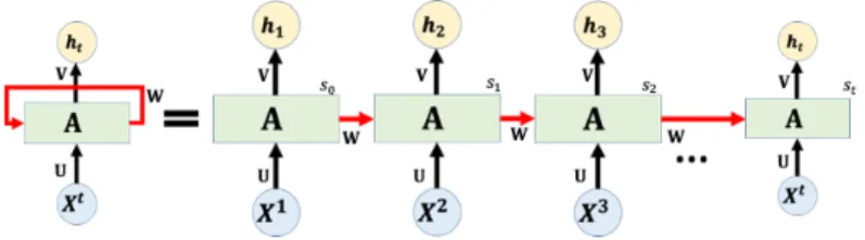
Recurrent Neural Networks (RNN) are designed to handle dependent inputs. This is the case when dealing with text, since a change in the order of words induce a change of meaning of a sentence. Therefore, where conventional neural networks consider that input and output data are independent, RNNs consider an information sequence. A representation of a RNN is provided in Figure 4.
Figure 4: A unrolled recurrent neural network and the unfolding representation in time of the computation involved in its forward computation.
According to this diagram, the different (embedded) words (or n−grams) constituting a report, pass successively into the network A. The t−h network produces an output (the final one constituting the prediction), but also a memory cell ct which is sent to the
next block. Hence, each single network uses a regular input (that is an embedded word), plus the information coming from the memory cell. This memory cell is the way to keep track on previous information. The most simple way to keep this information would be to identify the memory cell with the output of each network. Hence, the t−th network uses the information from the past in the sense that it take advantage of the prediction
done at the previous step. Nevertheless, this could lead to a fade of the contribution of the first words of the report, while they could be determinant.
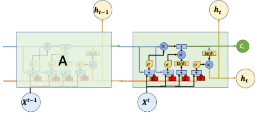
To circumvent this issue, one can turn at Long Short Term Memory (LSTM) networks have been introduced by [18]. They can be considered as a particular class of RNN with a design which allows to keep track of the information in a more flexible way. The purpose of LSTM is indeed to introduce a properly designed memory cell whose content evolves with t to keep relevant information through time (and ”forget” irrelevant).
As RNN, LSTM are successive blocks of networks. Each block can be described by Figure 5. The specificity of LSTM is the presence of a ”cell” ct which differs from the
output ht, and which can be understood as a channel to convey context information that
may be relevant to compute the following output ht+1 in the next block of the network.
The information contained in the cell passes through three gates. These so-called gates are simple operations that permit to keep, add or remove information to the memory cell.
Figure 5: Synthetic description of a block of a Long Short Term Memory network.
gate. This means that each component of the vector ctis multiplied by a number between
0 and 1 (contained in a vector ft), which allows to keep (value close to 1) or suppress
(value close to 0) the information contained in each component of ct. This vector ft is
computed from the new input xt and the output of the previous block ht−1.
Next, the modified memory cell enters an additive gate. This gate is used to add information. The added information is a vector ˜Ct, again computed from the input xt
and the previous output ht−1. This produces the updated memory cell that passes through
the next block.
Moreover, this memory cell is transformed and combined with (xt, ht−1) through the
third step, to produce a new output.
To summarize, the following set of operations are performed in each unit (here, σ denotes the classical sigmoid function, and [xt, ht−1] the concatenation of the vectors xt
and ht):
• Compute ut= σ(θ0[xt, ht−1]+b0), vt= σ(θ1[xt, ht−1]+b1), and wt= tanh(θ2[xt, ht−1]+
b2).
• The updated value of the memory cell is ct= ut× ct−1+ vt× wt.
• The new output is ht = σ(θ3[xt, ht−1] + b3) × tanh(ct).
5
Real data analysis
This section is devoted to a real data analysis. The aim is to predict a severity indicator of a claim (which is known only when the claim is fully settled) from expert reports. The main difficulty stands in the fact that the proportion of ”severe” claims that require a specific response is quite low. In section 5.1, we present the structure of the database and its specificities. Section 5.2 is devoted to the inventory of the different network structures and embedding methods that we use. The performance indicators that can be used to assess the quality of the method are shown in section 5.3. The results and discussion is made in section 5.4.
5.1
Description of the database
The database we consider gathers 113072 claims from a French insurer, and corresponding expert reports describing the circumstances. These reports have been established at the
Categories min mean var median max Standard claims (uncensored) 0 1 1 0,75 16.3 Extreme claims (uncensored) 0,25 3.83 6,93 3,08 16.3 Standard claims (after KM) 0 1.25 2.26 0,83 16.3 Extreme claims (after KM) 0,25 5.24 11.7 4.17 16.3
Table 1: Empirical statistics on the variable T, before and after correction by Kaplan-Meier weights (”after KM”). The category ”Extreme claims” corresponds to the situation where I = 1 for x = 3% of the claims, while ”Standard claims” refers to the 97% lower part of the distribution of the final amount.
opening of the claim, and do not take into account counter-expertises. Among these claims, 23% are still open (censored) at the date of extraction. Empirical statistics on the duration of a claim T are shown in Table 1.
For the claims that are closed, different severity indicators are known. These severity indicators have been previously computed from the final amount of the claim: I = 1 if the claim amount exceeds some quantile of the distribution of the amount, corresponding to the x% upper part of the distribution. In the situation we consider, this percentage x ranges from 1.5 to 7, which means that we focus on relatively rare events, since I = 0 for the vast majority of the claims.
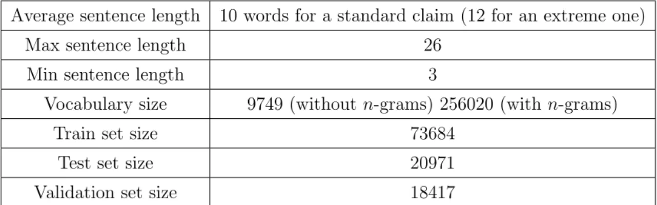
Some elements about the structure of the reports are summarized in Table 2 below. To get a first idea of which terms in the report could indicate severity, Table 3 shows which are the most represented words, distinguishing between claims with I = 1 and claims with I = 0.
In both cases, the two most frequent words are ”insurer” and ”third party”, which have to be linked with the guarantee involved. For extreme claims, we notice a frequent presence of a term related to a victim, for example motorcycle, or pedestrian. In addition there are also words related to the severity of the condition of a victim, such as injured or deceased. Moreover, two verbs are present in our top, ”to ram” (we used this translation of the French verb ”percuter”) and ”to hit” (in French, ”frapper”), which are related to some kind of violence of the event. On the other hand, for ”standard” claims, the most frequent words are related to the car. Hence, reports on extreme claims use the lexical field of bodily damage, while the others use the terminology related to material damage.
Average sentence length 10 words for a standard claim (12 for an extreme one) Max sentence length 26
Min sentence length 3
Vocabulary size 9749 (without n-grams) 256020 (with n-grams)
Train set size 73684
Test set size 20971
Validation set size 18417
Table 2: Summarized characteristics of the reports. The dataset is split into the train set (containing the observations used to fit the parameter of the network), the validation set (used to tune the hyper-parameters), and the test set (used to measure the quality of the model). The vocabulary size ”with n−grams” is the total of 1−grams, 2−grams and 3−grams.
5.2
Hyperparameters of the networks and type of embedding
Let us recall that our procedure is decomposed into three steps:
• A preliminary treatment to correct censoring (Kaplan-Meier weighting); • Embedding (determination of some appropriate metric between words);
• Prediction, using the embedded words as inputs of a neural network. Depending on the embedding strategy, the prediction phase is either disconnected from the embedding (static method) or done at the same time (after a FastText initialization, non-static method, or a random initialization, random method).
For the last phase, we use LSTM and CNN described in section 4. For each of these architectures, we compare the different variations (static, non-static and random). The static and non-static classes of method are expected to behave better, taking advantage of a pre-training via FastText. For the LSTM networks, we consider two cases: when the words are decomposed into n−grams (n = 1, 2, 3), or without considering n−grams. In each case, the idea is to measure the influence of the different rebalancing strategies.
The weights in each of the networks we consider are optimized using the Adagrad optimizer, see [13]. Training is done through stochastic gradient descent over shuffled mini-batches with the Adagrad update rule. The architecture and hyper-parameters of the LSTM and CNN are shown in Table 4 and Figure 7 and 8 below. The codes are available on https://github.com/isaaccs/Insurance-reports-through-deep-neural-networks.
Rank Extreme Normal 1 insurer 90% insurer 87% 2 third party 56% third party 61% 3 injured 38% front 46% 4 to ram 30% way 41% 5 to hit 24% backside 40% 6 motorcycle 18% left 20% 7 driver 17% right 18% 8 pedestrian 16% side 17% 9 inverse 15% to shock 14% 10 deceased 13% control 10%
Table 3: Ranking of the words (translated from French) used in the reports, depending on the category of claims (Extreme corresponds to I = 1 and Standard to I = 0.)
CNN LSTM
dense size 1 400 500 dense size 2 250 300 penalized 0.001 0.004
NB filter 1024 not for LSTM filtersize [1,2] not for LSTM nb units not for CNN [256,128]
Figure 8: Representation of the LSTM network used in the real data analysis. The output of the network is followed by a multilayer perceptron.
5.3
Performance indicators
In this section, we describe the criteria that are used to compare the final results of our models. Due to the small proportion of observations such that I = 1, measuring the performance only by the well-predicted responses would not be adequate, since a model which would systematically predict 0 would be ensured to obtain an almost perfect score according to this criterion. Let us introduce some notations:
• TN is the number of negative examples (I = 0) correctly classified, that is ”True Negatives”.
• FP is the number of negative examples incorrectly classified as positive (I = 1), that is ”False Positives”.
• FN is the number of positive examples incorrectly classified as negative (”False Negatives”).
• TP is the number of positive examples correctly classified (”True Positives”). We then define Recall and Precision as,
Recall = T P T P + F N, Precision = T P
So Recall is the proportion of 1 that have been correctly predicted with respect to the total number of 1. For Precision, the number of correct predictions of 1 is compared to the total of 1-predicted observations. F1−score (see for example [2]) is a way to combine
these two measures, introducing F1 =
2 × Recall × P recision Recall + P recision .
The F1−score conveys the balance between the precision and recall.
Remark:
F1−score is a particular case of a more general family of measures defined as
Fβ =
(1 + β2) × Recall × P recision
Recall + β2× P recision ,
where β is a coefficient to adjust the relative importance of precision versus recall, de-creasing β leads a reduction of precision importance. In order to adapt the measure to cost-sensitive learning methods [10] proposed to rely on
β = c(1, 0)
c(0, 1), (5.1)
where c(1, 0) (resp. c(0, 1)) is the cost associated to the prediction of a False Negative (resp. of a False Positive). The rationale behind the introduction of such Fβ measure is
that misclassifying within the minority class is typically more expansive than within the majority class. Hence, considering the definition (5.1) of β, improving Recall will more affect Fβ than improving Precision. In our practical situation, it was difficult to define a
legitimate cost for such bad predictions, which explains why we only considered F1−score
among the family of Fβ−measures.
5.4
Results
As we already mention, I = 1 corresponds to a severe event, that is the loss associated with the claim corresponds to the x% upper part of the loss distribution. We made this proportion vary from 1.5% to 7% to see the sensitivity to this parameter. Table 5 shows the benefits of using the different resampling algorithms of section 2.3 in the case where the proportion of 1 in the sample is 3% (which is an intermediate scenario considering the range of values for x that we consider). The neural networks methods are benchmarked with a classical logistic predictor, and two other competing machine learning methodology
alternatives methodologies are combined with the FastText embedding (as in the static methods). Moreover, we apply the same resampling algorithms of section 2.3 to these methods.
Let us first observe that the network methodologies lead to a relatively good precision if one does not use rebalancing strategies. This is due to the fact that precision only measures the proportion of true positive among all the claims that have been predicted to be 1. Typically, the networks methodologies, in this case, predict correctly the ”obviously” severe claims, but miss lots of these severe claims. This explains why recall and F1−score
are much lower.
The rebalancing algorithm mostly benefit the machine learning methodologies. One also observes that the embedding methodologies based on FastText (static and non-static methods) leads to better performances. The performance of all techniques in terms of F1−score is not spectacular (in the sense that it is not close to 1), but this has to be related
with the complexity of the problem (predicting a relatively rare class of events). Compared to the basic logistic method (after embedding), the best network (LSTM without consid-ering n grams, with the lightly balanced bagging algorithm) leads to an improvement of 20% in terms of F1−score.
Let us also observe that the LSTM network architecture which does not rely on n−grams behaves better than the LSTM which actually uses these n−grams. This may be counterintuitive, since the use of n−grams is motivated by the idea that one could use them to take the context of the use of a word into account. Nevertheless, considering n−grams increases the number of parameters of the network, while context information is already present in the embedding methodologies. On the other hand, CNN methods have lower performance than LSTM ones, but the performances stay in the same range (with a computation time approximatively 4 times smaller to fit the parameters of the network).
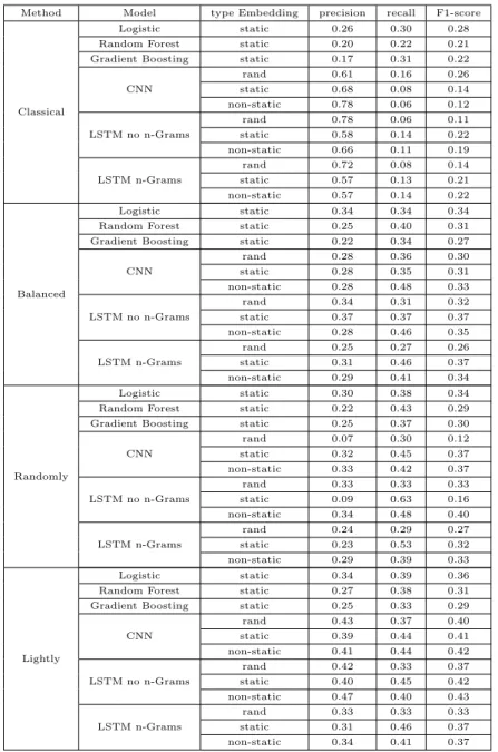
Method Model type Embedding precision recall F1-score
Classical
Logistic static 0.26 0.30 0.28 Random Forest static 0.20 0.22 0.21 Gradient Boosting static 0.17 0.31 0.22
CNN rand 0.61 0.16 0.26 static 0.68 0.08 0.14 non-static 0.78 0.06 0.12 LSTM no n-Grams rand 0.78 0.06 0.11 static 0.58 0.14 0.22 non-static 0.66 0.11 0.19 LSTM n-Grams rand 0.72 0.08 0.14 static 0.57 0.13 0.21 non-static 0.57 0.14 0.22 Balanced Logistic static 0.34 0.34 0.34 Random Forest static 0.25 0.40 0.31 Gradient Boosting static 0.22 0.34 0.27
CNN rand 0.28 0.36 0.30 static 0.28 0.35 0.31 non-static 0.28 0.48 0.33 LSTM no n-Grams rand 0.34 0.31 0.32 static 0.37 0.37 0.37 non-static 0.28 0.46 0.35 LSTM n-Grams rand 0.25 0.27 0.26 static 0.31 0.46 0.37 non-static 0.29 0.41 0.34 Randomly Logistic static 0.30 0.38 0.34 Random Forest static 0.22 0.43 0.29 Gradient Boosting static 0.25 0.37 0.30
CNN rand 0.07 0.30 0.12 static 0.32 0.45 0.37 non-static 0.33 0.42 0.37 LSTM no n-Grams rand 0.33 0.33 0.33 static 0.09 0.63 0.16 non-static 0.34 0.48 0.40 LSTM n-Grams rand 0.24 0.29 0.27 static 0.23 0.53 0.32 non-static 0.29 0.39 0.33 Lightly Logistic static 0.34 0.39 0.36 Random Forest static 0.27 0.38 0.31 Gradient Boosting static 0.25 0.33 0.29
CNN rand 0.43 0.37 0.40 static 0.39 0.44 0.41 non-static 0.41 0.44 0.42 LSTM no n-Grams rand 0.42 0.33 0.37 static 0.40 0.45 0.42 non-static 0.47 0.40 0.43 LSTM n-Grams rand 0.33 0.33 0.33 static 0.31 0.46 0.37 non-static 0.34 0.41 0.37
Table 5: Influence of the constrained bagging algorithms of section 2.3. For ”Classical,” no rebalancing algorithm has been used. ”Balanced” corresponds to algorithm 3 with an equal proportion of 1 and 0 in each sample. ”Randomly” corresponds to algorithm 4 with an equal proportion (in average) of 1 and 0 in each sample. ”Lightly” corresponds to algorithm 4 with 10% of 1 (in average) in each sample.
Table 6 shows the influence of the proportion x on the performance (we only report a selected number of methods for the sake of brevity. We observe that the performance of the logistic method decreases with the proportion of 1 contained in the sample. On the
Extreme Values Percent Model type Embedding precision recall f1-score 1.5% Logistic static 0.19 0.24 0.21 CNN rand 0.38 0.41 0.39 static 0.49 0.36 0.41 non-static 0.40 0.42 0.41 LSTM rand 0.42 0.33 0.37 static 0.34 0.47 0.39 non-static 0.47 0.40 0.43 3.5% Logistic static 0.27 0.35 0.30 CNN rand 0.39 0.47 0.43 static 0.37 0.48 0.42 non-static 0.35 0.45 0.40 LSTM rand 0.33 0.37 0.34 static 0.35 0.49 0.40 non-static 0.34 0.49 0.40 5% Logistic static 0.25 0.42 0.31 CNN rand 0.41 0.44 0.42 static 0.40 0.46 0.43 non-static 0.42 0.45 0.44 LSTM rand 0.22 0.31 0.26 static 0.37 0.49 0.42 non-static 0.43 0.37 0.40 7% Logistic static 0.29 0.45 0.35 CNN rand 0.40 0.47 0.43 static 0.43 0.46 0.44 non-static 0.38 0.46 0.41 LSTM rand 0.32 0.34 0.33 static 0.42 0.41 0.42 non-static 0.43 0.40 0.41
Table 6: Performance of the different methodologies (combined with the different embed-ding technics). The first column indicates the percentage of 1 in the sample.
6
Conclusion
In this paper, we proposed a detailed methodology to perform automatic analysis of text reports in insurance, in view of predicting a rare event. In our case, the rare event is a particularly severe claim. This question of clustering such claim is of strategic impor-tance, since it allows to operate a particular treatment of the claims that are identified as ”extreme”. Four steps of our method are essential:
• correction of censoring via survival analysis techniques;
• compensation of the rarity of the severe events via rebalancing bagging techniques; • a proper representation of the words contained in the reports via an appropriate
embedding technique;
• the choice of a proper neural network architecture.
Long Short Term Memory networks, associated with a performant embedding method, appear to be promising tools to perform this task. Nevertheless, learning rare events is
still a hard task, especially in such insurance problem where the volume of data is limited. The integration of additional variables to increase the information on the claims should be essential to improve the prediction. Moreover, let us mention that, in this work, we only considered information available at the opening of the claim to predict its outcome. For long development branches, the incorporation of updated information on the evolution of the claims could be determinant and should be incorporated in the methodology.
7
Appendix
7.1
Typical choices of activation functions for neural networks
A list of typical activation functions is provided in Table 7.
Name Function
Sigmoid function σ : R → [0, 1] x 7→ 1
1+e−x
Hyperbolic tangent tanh : R → [−1, 1] x 7→ 2σ(2x) + 1 ReLU f : R → R + x 7→ max(0, x) Leaky ReLU f : R → R + x 7→ αx1x≤0+ x1x>0
where α is a small constant Swish function[32] σ : R → [0, 1]
x 7→ x 1+e−x
Table 7: Typical choices of activation functions.
7.2
Additional type of layers in a CNN
Zero-padding. Zero-padding is the simplest way to avoid diminishing too much the dimension of the input when going deeper into the network. As we can see above in Figure 3, a convolution step will produce an output C of smaller dimension than A. Moreover, when dealing with our text data, it is useful to control the size of our inputs. Let us recall that we want to automatically analyse reports to predict the severity of a claim. These reports do not all have the same size in terms of words. Zero-padding creates a larger matrix by adding zeros on the boundaries, as shown in the example of Figure 9. Similar issues are present when dealing with images that may not all have the same number of pixels.
Figure 9: Zero-padding
Pooling Step. Pooling steps work similarly as convolution layers, but applying locally a function that may not be linear. An example is shown in Figure 10.
Figure 10: Example of a Pooling Layer: each function is applied to a moving square of input coefficients of size 2x2.
Let us note that, in the example of Figure 10, the functions ’Average’ and ’Sum’ may be seen as linear filters, as in Figure 3 (for example, function ’Sum’ is related to a filter B whose coefficients are all 1). The only difference is that the parameters of a convolution layer evolves through the calibration process of the network, while the coefficients of a pooling layer are fixed.
7.3
Hyperparameters
8 lists the range of values on which the optimization has been done. The Embedding dimension denotes the dimension N after reduction of the vocabulary V. Batch size is a parameter used in the Batch Gradient Descent (used in the algorithm of optimization of the weights of the networks), see [5]. The number of hidden layers refer to the final multilayer perceptron block used at the output of LSTM and CNN networks.
Hyperparameter Grid Embedding dimension 32 to 126 n-grams characters for embedding 1 to 5
Batch size 8 to 256 Number of hidden layers 1 to 5 Number of neurons in each layer 450 to 50
Number of filters for the CNN 32 to 1024 Size of the filters 1 to 5
Table 8: Range of values on which the hyperparameters have been optimized. All the codes are available at the following url:
https://github.com/isaaccs/Insurance-reports-through-deep-neural-networks.
References
[1] Charu C Aggarwal and ChengXiang Zhai. Mining text data. Springer Science & Business Media, 2012.
[2] Josephine Akosa. Predictive accuracy: A misleading performance measure for highly imbalanced data. In Proceedings of the SAS Global Forum, 2017.
[3] Michael G Akritas et al. The central limit theorem under censoring. Bernoulli, 6(6):1109–1120, 2000.
[4] Neena Aloysius and M Geetha. A review on deep convolutional neural networks. In 2017 International Conference on Communication and Signal Processing (ICCSP), pages 0588–0592. IEEE, 2017.
[5] Yoshua Bengio. Practical recommendations for gradient-based training of deep ar-chitectures. In Neural networks: Tricks of the trade, pages 437–478. Springer, 2012.
[6] Michael W Berry and Malu Castellanos. Survey of text mining. Computing Reviews, 45(9):548, 2004.
[7] Piotr Bojanowski, Edouard Grave, Armand Joulin, and Tomas Mikolov. Enriching word vectors with subword information. arXiv preprint arXiv:1607.04606, 2016. [8] Piotr Bojanowski, Edouard Grave, Armand Joulin, and Tomas Mikolov. Enriching
word vectors with subword information. Transactions of the Association for Compu-tational Linguistics, 5:135–146, 2017.
[9] Leo Breiman. Bagging predictors. Machine learning, 24(2):123–140, 1996.
[10] Nitesh V Chawla, Kevin W Bowyer, Lawrence O Hall, and W Philip Kegelmeyer. Smote: synthetic minority over-sampling technique. Journal of artificial intelligence research, 16:321–357, 2002.
[11] Jianpeng Cheng, Li Dong, and Mirella Lapata. Long short-term memory-networks for machine reading. arXiv preprint arXiv:1601.06733, 2016.
[12] Turkan Erbay Dalkilic, Fatih Tank, and Kamile Sanli Kula. Neural networks ap-proach for determining total claim amounts in insurance. Insurance: Mathematics and Economics, 45(2):236–241, 2009.
[13] John Duchi, Elad Hazan, and Yoram Singer. Adaptive subgradient methods for online learning and stochastic optimization. Journal of machine learning research, 12(Jul):2121–2159, 2011.
[14] Martin Ellingsworth and Dan Sullivan. Text mining improves business intelligence and predictive modeling in insurance. Information Management, 13(7):42, 2003. [15] Jerome Friedman, Trevor Hastie, and Robert Tibshirani. The elements of statistical
learning, volume 1. Springer series in statistics Springer, Berlin, 2001.
[16] Guillaume Gerber, Yohann Le Faou, Olivier Lopez, and Michael Trupin. The impact of churn on client value in health insurance, evaluation using a random forest under random censoring. 2018.
[17] Trevor Hastie, Robert Tibshirani, and Jerome Friedman. The elements of statistical learning: data mining, inference, and prediction. Springer Science & Business Media,
[18] Sepp Hochreiter and J¨urgen Schmidhuber. Long short-term memory. Neural compu-tation, 9(8):1735–1780, 1997.
[19] Armand Joulin, Edouard Grave, Piotr Bojanowski, Matthijs Douze, H´erve J´egou, and Tomas Mikolov. Fasttext.zip: Compressing text classification models. arXiv preprint arXiv:1612.03651, 2016.
[20] Armand Joulin, Edouard Grave, Piotr Bojanowski, and Tomas Mikolov. Bag of tricks for efficient text classification. arXiv preprint arXiv:1607.01759, 2016.
[21] Edward L Kaplan and Paul Meier. Nonparametric estimation from incomplete ob-servations. Journal of the American statistical association, 53(282):457–481, 1958. [22] Yoon Kim. Convolutional neural networks for sentence classification. arXiv preprint
arXiv:1408.5882, 2014.
[23] Douglas M Kline and Victor L Berardi. Revisiting squared-error and cross-entropy functions for training neural network classifiers. Neural Computing & Applications, 14(4):310–318, 2005.
[24] Inna Kolyshkina and Marcel van Rooyen. Text mining for insurance claim cost prediction. In Data Mining, pages 192–202. Springer, 2006.
[25] Alex Krizhevsky, Ilya Sutskever, and Geoffrey E Hinton. Imagenet classification with deep convolutional neural networks. In Advances in neural information processing systems, pages 1097–1105, 2012.
[26] Tsung-Yi Lin, Priya Goyal, Ross Girshick, Kaiming He, and Piotr Doll´ar. Focal loss for dense object detection. In Proceedings of the IEEE international conference on computer vision, pages 2980–2988, 2017.
[27] Olivier Lopez. A censored copula model for micro-level claim reserving. Insurance: Mathematics and Economics, 87:1–14, 2019.
[28] Olivier Lopez, Xavier Milhaud, Pierre-E Th´erond, et al. Tree-based censored regres-sion with applications in insurance. Electronic journal of statistics, 10(2):2685–2716, 2016.
[29] Tom´aˇs Mikolov, Martin Karafi´at, Luk´aˇs Burget, Jan ˇCernock`y, and Sanjeev Khudan-pur. Recurrent neural network based language model. In Eleventh annual conference of the international speech communication association, 2010.
[30] Sankaran Panchapagesan, Ming Sun, Aparna Khare, Spyros Matsoukas, Arindam Mandal, Bj¨orn Hoffmeister, and Shiv Vitaladevuni. Multi-task learning and weighted cross-entropy for dnn-based keyword spotting. In Interspeech, volume 9, pages 760– 764, 2016.
[31] Xueheng Qiu, Le Zhang, Ye Ren, Ponnuthurai N Suganthan, and Gehan Ama-ratunga. Ensemble deep learning for regression and time series forecasting. In 2014 IEEE symposium on computational intelligence in ensemble learning (CIEL), pages 1–6. IEEE, 2014.
[32] Prajit Ramachandran, Barret Zoph, and Quoc V. Le. Searching for activation func-tions, 2017.
[33] Xin Rong. word2vec parameter learning explained. arXiv preprint arXiv:1411.2738, 2014.
[34] Olaf Ronneberger, Philipp Fischer, and Thomas Brox. U-net: Convolutional net-works for biomedical image segmentation. In International Conference on Medical image computing and computer-assisted intervention, pages 234–241. Springer, 2015. [35] Andrea Rotnitzky and James M Robins. Inverse probability weighting in survival
analysis. Wiley StatsRef: Statistics Reference Online, 2014.
[36] David E Rumelhart, Geoffrey E Hinton, and Ronald J Williams. Learning represen-tations by back-propagating errors. nature, 323(6088):533–536, 1986.
[37] Aditya Rizki Saputro, Hendri Murfi, and Siti Nurrohmah. Analysis of deep neural networks for automobile insurance claim prediction. In International Conference on Data Mining and Big Data, pages 114–123. Springer, 2019.
[38] Winfried Stute. The central limit theorem under random censorship. The Annals of Statistics, pages 422–439, 1995.
[39] Winfried Stute. Distributional convergence under random censorship when covari-ables are present. Scandinavian journal of statistics, pages 461–471, 1996.
[40] Winfried Stute. Nonlinear censored regression. Statistica Sinica, pages 1089–1102, 1999.
[41] Mario V W¨uthrich. Neural networks applied to chain–ladder reserving. European Actuarial Journal, 8(2):407–436, 2018.
[42] Matthew D Zeiler. Adadelta: an adaptive learning rate method. arXiv preprint arXiv:1212.5701, 2012.