A Chemical and Kinematical Analysis of the Intermediate-age Open Cluster IC 166 from APOGEE and Gaia DR2

(1)

HAL Id: hal-02023251

https://hal.archives-ouvertes.fr/hal-02023251

Submitted on 8 Dec 2020

HAL is a multi-disciplinary open access

archive for the deposit and dissemination of

sci-entific research documents, whether they are

pub-lished or not. The documents may come from

teaching and research institutions in France or

abroad, or from public or private research centers.

L’archive ouverte pluridisciplinaire HAL, est

destinée au dépôt et à la diffusion de documents

scientifiques de niveau recherche, publiés ou non,

émanant des établissements d’enseignement et de

recherche français ou étrangers, des laboratoires

publics ou privés.

A Chemical and Kinematical Analysis of the

Intermediate-age Open Cluster IC 166 from APOGEE

and Gaia DR2

J. Schiappacasse-Ulloa, B. Tang, J. Fernández-Trincado, O. Zamora, D.

Geisler, P. Frinchaboy, M. Schultheis, F. Dell’agli, S. Villanova, T. Masseron,

et al.

To cite this version:

J. Schiappacasse-Ulloa, B. Tang, J. Fernández-Trincado, O. Zamora, D. Geisler, et al.. A Chemical

and Kinematical Analysis of the Intermediate-age Open Cluster IC 166 from APOGEE and Gaia

DR2. Astronomical Journal, American Astronomical Society, 2018, 156 (3), pp.94.

�10.3847/1538-3881/aad048�. �hal-02023251�

(2)

6_{Department of Physics and Astronomy, Texas Christian University, Fort Worth, TX 76129, USA} 7

Laboratoire Lagrange, Université Côte d’Azur, Observatoire de la Côte d’Azur, CNRS, Bd de l’Observatoire, F-06304 Nice, France 8

ELTE Eötvös Loránd University, Gothard Astrophysical Observatory, Szombathely, Hungary 9

Observatório Nacional, 20921-400 Sao Cristóvao, Rio de Janeiro, Brazil 10

New Mexico State University, Las Cruces, NM 88003, USA 11

Steward Observatory, University of Arizona, 933 North Cherry Avenue, Tucson, AZ 85721, USA 12

National Optical Astronomy Observatories, Tucson, AZ 85719, USA 13

Centro de Investigaciones de Astronomía, AP 264,Mérida 5101-A, Venezuela 14

Departamento de Fisica, Facultad de Ciencias Exactas, Universidad Andres Bello Av. Fernandez Concha 700, 7591538 Las Condes, Santiago, Chile 15

Instituto Milenio de Astrofísica, Santiago, Chile 16

Vatican Observatory, V00120 Vatican City State, Italy

17_{Department of Physics and Astronomy, The University of Utah, Salt Lake City, UT 84112, USA} 18

Instituto de Astronomía, Universidad Nacional Autónoma de México, Apdo. Postal 70264, México D.F., 04510, México 19

Universidade de São Paulo, IAG, Rua do Matão 1226, Cidade Universitária, 05508-900, São Paulo, Brazil 20

Instituto de Astrofísica, Pontiﬁcia Universidad Católica de Chile, Av. Vicuña Mackenna 4860, 782-0436 Macul, Santiago, Chile 21

Apache Point Observatory and New Mexico State University, P.O. Box 59, Sunspot, NM, 88349-0059, USA 22

Unidad de Astronomía, Universidad de Antofagasta, Avenida Angamos 601, Antofagasta 1270300, Chile 23

Universidad de Chile, Av. Libertador Bernardo O’Higgins 1058, Santiago De Chile 24

Departamento de Física, Facultad de Ciencias, Universidad de La Serena, Cisternas 1200, La Serena, Chile Received 2018 January 25; revised 2018 June 24; accepted 2018 June 27; published 2018 August 10

Abstract

IC 166 is an intermediate-age open cluster(OC) (∼1 Gyr) that lies in the transition zone of the metallicity gradient in the outer disk. Its location, combined with our very limited knowledge of its salient features, make it an interesting object of study. We present theﬁrst high-resolution spectroscopic and precise kinematical analysis of IC 166, which lies in the outer disk with RGC∼12.7 kpc. High-resolution H-band spectra were analyzed using observations from

the SDSS-IV Apache Point Observatory Galactic Evolution Experiment survey. We made use of the Brussels Automatic Stellar Parameter code to provide chemical abundances based on a line-by-line approach for up to eight chemical elements(Mg, Si, Ca, Ti, Al, K, Mn, and Fe). The α-element (Mg, Si, Ca, and whenever available Ti) abundances, and their trends with Fe abundances have been analyzed for a total of 13 high-likelihood cluster members. No signiﬁcant abundance scatter was found in any of the chemical species studied. Combining the positional, heliocentric distance, and kinematic information, we derive, for theﬁrst time, the probable orbit of IC 166 within a Galactic model including a rotating boxy bar, and found that it is likely that IC 166 formed in the Galactic disk, supporting its nature as an unremarkable Galactic OC with an orbit bound to the Galactic plane.

Key words: Galaxy: abundances– Galaxy: kinematics and dynamics – open clusters and associations: individual (IC 166)

1. Introduction

Galactic open clusters(OCs) have a wide age range, from 0 to almost 10 Gyr, and they are spread throughout the Galactic

disk; therefore, they are widely used to characterize the properties of the Galactic disk, such as the morphology of the spiral arms of the Milky Way(MW; Bonatto et al.2006; van den Bergh2006; Vázquez et al. 2008), the stellar metallicity gradient (e.g., Janes 1979; Geisler et al. 1997; Frinchaboy et al.2013; Cunha et al.2016; Jacobson et al. 2016), the age– metallicity relation in the Galactic disk(Carraro & Chiosi1994; Carraro et al. 1998; Salaris et al. 2004; Magrini et al.2009), and the Galactic disk star formation history (de la Fuente Marcos & de la Fuente Marcos2004). OCs are thus crucial in

25

Premium Postdoctoral Fellow of the Hungarian Academy of Sciences.

Original content from this work may be used under the terms of theCreative Commons Attribution 3.0 licence. Any further distribution of this work must maintain attribution to the author(s) and the title of the work, journal citation and DOI.

(3)

developing a more comprehensive understanding of the Galactic disk.

OCs are generally considered to be archetypal examples of a simple stellar population (Deng & Xin 2007), because individual member stars of each OC are essentially homo-geneous, both in age, dynamically (similar radial velocities (RVs) and proper motions) and chemically (similar chemical patterns), greatly facilitating our ability to derive global cluster parameters from studying limited samples of stars. However, possible small inhomogeneous chemical patterns in OCs have been recently suggested, though only at the 0.02 dex level(e.g., Hyades; Liu et al.2016).

IC 166 (l=130°.071, b=−0°.189) is an intermediate-age OC (∼1.0 Gyr; Vallenari et al. 2000; Subramaniam & Bhatt 2007) located in the outer part of the Galactic disk (RGC≈13 kpc). Previous literature studies of this cluster used

mainly photometric and low-resolution spectroscopic data. Detailed photometric studies were carried out by Subramaniam & Bhatt(2007), Vallenari et al. (2000), and Burkhead (1969) in order to estimate its age, extinction, and distance. In addition, Dias et al. (2014), Dias et al. (2002), Loktin & Beshenov (2003), and Twarog et al. (1997) have derived proper motions in the IC 166ﬁeld. Friel & Janes (1993) and Friel et al. (1989) have estimated the RV and metallicity of IC 166 from low-resolution spectroscopic data. In this work, we will for theﬁrst time provide an extensive, detailed investigation of its chemical abundances as well as its orbital parameters.

OCs are continuously inﬂuenced by destructive effects such as (1) evaporation (Moyano Loyola & Hurley 2013), where some members reach the escape velocity after intracluster stellar encounters with other members, and/or via interaction with the Galactic tidalﬁeld, and (2) close encounters with giant interstellar clouds (Gieles & Renaud 2016). Interactions with giant molecular clouds along their orbit in the Galactic disk have a high probability to eventually disrupt star clusters (Lamers et al.2005; Gieles et al.2006; Lamers & Gieles2006). These effects can lead to the dissolution of a typical OC in ∼108_years_(Friel₂₀₁₃_{). Thus, intermediate-age and old OCs}

(1.0 Gyr) are rare by nature and are of great interest (Donati et al. 2014; Friel et al. 2014; Magrini et al. 2015; Tang et al. 2017). As these effects are generally less severe in the outer disk, OCs there have a higher chance of survival, providing a great opportunity to study this part of the Galaxy both chemically and dynamically. Moreover, IC 166 is located close to the region where a break in the metallicity gradient is suggested (between 10 and 13 kpc from the Galactic center; Yong et al. 2012; Frinchaboy et al.2013; Reddy et al. 2016). Accurate determination of the cluster’s metallicity is helpful to constrain the nature of this possible break.

Large-scale multi-object spectroscopic surveys, such as the Apache Point Observatory Galactic Evolution Experiment (APOGEE; Majewski et al.2017) provide a unique opportunity to study a wide gamut of light-/heavy-elements in the H-band in hundreds of thousands of stars in a homogeneous way (García Pérez et al.2016; Hasselquist et al.2016; Cunha et al.2017). In this work, we provide an independent abundance determination of several chemical species in the OC IC 166 using the Brussels Automatic Code for Characterizing High accUracy Spectra (BACCHUS; Masseron et al.2016), and compare them with the Apogee Stellar Parameter and Chemical Abundances Pipeline (ASPCAP; García Pérez et al. 2016).

This paper is organized as follows. Cluster membership selection is described in Section2. In Section3, we determine the atmospheric parameters for our selected members. In Section 4, we present our derived chemical abundances. A detailed description of the orbital elements is given in Section5. We present our conclusions in Section6.

2. Target Selection

The APOGEE(Majewski et al. 2017) is one of the projects operating as part of the Sloan Digital Sky Survey IV (Blanton et al. 2017; Abolfathi et al. 2018), aiming to characterize the MW Galaxy’s formation and evolution through a precise, systematic and large-scale kinematic and chemical study. The APOGEE instrument is a near-infrared (λ=1.51–1.70 μm) high-resolution(R≈22,500) multi-object spectrograph (Wilson et al. 2012) mounted at the SDSS 2.5 m telescope (Gunn et al. 2006), with a copy now operating in the South at Las Campanas Observatory—the 2.5 m Irénée du Pont telescope. The APOGEE survey has observed more than 270,000 stars across all of the main components of the MW (Zasowski et al. 2013, 2017), achieving a typical spectral signal-to-noise ratio (S/N)>100 per pixel. The latest data release (DR14; Abolfathi et al.2018) includes all of the APOGEE-1 data and APOGEE data taken between 2014 July and 2016 July. A number of candidate member stars of the OC IC 166 were observed by the APOGEE survey, and their spectra were released for the ﬁrst time as part of the DR14 (Abolfathi et al.2018).

We selected a sample of potential stellar members for IC 166 using the following high quality control cuts:

1. Spatial Location: We focus on stars that are located inside half of the tidal radius(rt/2), where rt= 35.19±6.10 pc

(Kharchenko et al. 2012). This can minimize Galactic foreground stars. Figure1shows the spatial distribution of 21 highest likelihood cluster members inside half of the tidal radius, highlighted with red dots, for ourﬁnal sample of likely cluster members. Stars with projected distances from the center larger than half of the tidal radius were removed, in order to obtain a cleaner sample, relatively uncontaminated by disk stars.

2. RV and Metallicity: We further selected member stars using their RVs. Figure 2 shows the RV versus [Fe/H] distribution of the stars in the APOGEE observationﬁeld of IC 166. Clearly, twenty out of twenty-one likely cluster members that we selected using only spatial information show a RV peak around −40 km s−1, except one with much lower RV (≈−96 km s−1). The other 20 cluster members show a mean RV of −40.50±1.66 km s−1. Applying a 3σ limit, we excluded stars outside of −40.50±3×1.66 km s−1 _{(gray region in Figure} ₂_).

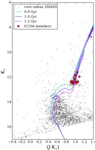
Twenty stars were selected as likely members. After the spatial location and RV selection, their membership status is further scrutinized byfiltering out all stars failing to meet the metallicity criteria. We adopt the calibrated metallicity from DR14 APOGEE/ASPCAP as a first guess in order to derive a cleaner sample of cluster stars. We identified a metallicity peak at−0.06 dex; thus, stars with metallicities differing by more than 0.03 dex from this mean were removed. Fifteen stars were left as likely members. 3. CMD Location: The left panel of Figure 3 shows the

(4)

lying inside one half of the tidal radius. Our selected APOGEE sample clearly lies near the red clump, consistent with the red clump observed in the Teffversus

log(g) plane (right panel of Figure 3). Interestingly,

Vallenari et al.(2000) also reported a clear red clump in IC 166, but did notfind evidence of RGB stars. Two out of the fifteen stars selected previously were located away from the red clump of IC 166. These stars were also removed from further consideration, although isochrones indicate they could well be upper RGB members. The isochrones shown in Figure3were selected from PARSEC (Bressan et al. 2012) for [Fe/H]=−0.06 dex and ages (0.8, 1.0 and 1.2 Gyr; Vallenari et al.2000; Subramaniam & Bhatt2007) to match the metallicity and age reported for this cluster. The candidates are in good agreement with the selected isochrones. The PARSEC isochrones used have been fitted by eye to the luminosity and color of the red clump stars. There is a small discrepancy in the location of de-reddened red clump stars found using the optical photometry and the Teffversus log(g) diagram.

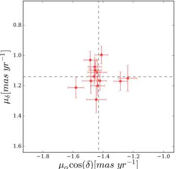
Lastly, we examine the newly measured proper motions from Gaia DR2 (Gaia Collaboration et al. 2018; Lindegren et al. 2018) of the APOGEE/IC 166 candidates. Figure 4 shows the proper motion diagram for IC 166. The dashed lines show the estimated mean proper motion value for IC 166. Gaia DR2 reveals that the selected stars in this study exhibit similar proper motions to each other, with a relatively small spread (<0.2 mas yr−1_{; see Figure} ₄_{), which are good enough for a}

precise orbit predictions of IC 166.

Figure 2.The APOGEE/DR14 RV vs. metallicity of stars in the field of the cluster(gray open circles) and our final sample (red dots). The gray regions show the upper and lower limits for the membership selection described in the text. The dotted lines show the mean RV and[Fe/H] of our final sample.

Figure 3.CMD of IC 166 using J and Ks magnitudes. Small gray points

represent stars observed by 2MASS inside of the rcore. Red dots represent our

potential members observed by APOGEE and black dots the two stars not passing our high quality cuts(see the text). Isochrones for 0.8 Gyr (sky-blue line), 1.0 Gyr (blue line), and 1.2 Gyr (magenta line) from PARSEC are also plotted.

Figure 1.On-sky distribution of the 13 highest likelihood cluster members analyzed in this work(red symbols) and within 17.6 arcmin (half of the tidal radius) of the center (red dashed line). The inner “x” symbol is the center of the cluster. Indicated with black open circles areﬁeld stars that were also observed by APOGEE. The large blue dashed circle shows the tidal radius of the cluster (35.19 arcmin), while the inner green dashed circle shows the core radius of the cluster.

(5)

Table1 shows the basic parameters of the stars that satisfy all the criteria previously mentioned, where raw Teffand log(g)

have been considered. These 13 stars will be considered as likely members of IC 166 and constitute our ﬁnal cluster sample.

3. Atmospheric Parameters and Abundance Determinations

For the stars observed with APOGEE and identiﬁed as members in Section 2, atmospheric parameters (Teff, log g,

[M/H], and ξ) were determined using the code FERRE (Allende Prieto et al. 2006) that compares theoretical spectra computed from MARCS atmosphere models (Gustafsson et al. 2008; Zamora et al. 2015) using the entire wavelength range, and minimizes the difference with the observed spectrum via a χ2 _{minimization. Our synthetic spectra were based on}

one-dimensional Local Thermodynamic Equilibrium (LTE) model atmospheres calculated with MARCS (Gustafsson et al.2008). The derived atmospheric parameters are listed in Table2.

It is important to note that we chose not to estimate the Teff

values from any empirical color–temperature relation; this

would be highly uncertain due to relatively large and likely differential reddening along the line of sight to IC 166, E B( -V)»0.80 (Subramaniam & Bhatt2007).

Figure 5 displays the main stellar parameters determined from FERRE/MARCS against those computed from ASP-CAP/KURUCZ (raw values), overplotted on the PARSEC isochrones (Bressan et al. 2012) with ages of 0.8, 1.0, and 1.2 Gyr. We notice that the raw (not post-calibrated) stellar parameters obtained via ASPCAP/KURUCZ are in fairly good agreement with the stellar parameters derived in this study

Table 1

Summary Table of Likely Members of IC 166

Apogee ID Tag R.A. Decl. J K %a

2M01514975+6150556 Star#1 27.957296 61.848778 13.417 12.360 ... 2M01515473+6148552 Star#2 27.978044 61.815334 13.403 12.393 95 2M01520770+6150058 Star#3 28.032106 61.834946 13.446 12.503 96 2M01521347+6152558 Star#4 28.056156 61.882183 13.487 12.462 ... 2M01521509+6151407 Star#5 28.062883 61.861309 13.118 12.129 84 2M01522060+6150364 Star#6 28.085842 61.843445 12.835 11.845 95 2M01522357+6154011 Star#7 28.098241 61.900307 13.262 12.327 96 2M01522953+6151427 Star#8 28.123055 61.861885 12.649 11.603 ... 2M01523324+6152050 Star#9 28.138523 61.868073 13.244 12.343 63 2M01523513+6154318 Star#10 28.146393 61.908844 13.326 12.409 ... 2M01524136+6151507 Star#11 28.172348 61.864094 13.385 12.445 93 2M01525074+6145411 Star#12 28.211422 61.76144 13.048 11.956 ... 2M01525543+6148504 Star#13 28.230962 61.814007 12.847 11.844 ... Note. a

Membership probability from Dias et al.(2014).

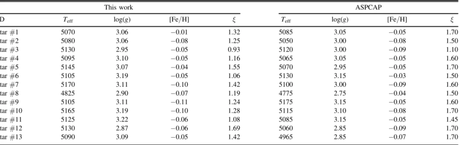
Table 2

Stellar Parameters Obtained from FERRE/MARCS

This work ASPCAP

ID Teff log(g) [Fe/H] ξ Teff log(g) [Fe/H] ξ

star#1 5070 3.06 −0.01 1.32 5085 3.05 −0.05 1.70 star#2 5080 3.06 −0.08 1.25 5050 3.00 −0.08 1.50 star#3 5130 2.95 −0.05 0.93 5120 3.00 −0.09 1.10 star#4 5095 3.10 −0.05 1.16 5065 3.05 −0.05 1.60 star#5 5145 3.07 −0.04 1.55 5070 2.95 −0.05 1.70 star#6 5105 3.19 −0.05 1.06 5130 3.15 −0.03 1.50 star#7 5170 3.11 −0.10 1.42 5100 3.00 −0.09 1.60 star#8 4825 2.90 −0.07 1.19 4775 2.75 −0.04 1.50 star#9 5105 3.11 −0.11 1.24 5175 3.15 −0.05 1.60 star#10 5165 3.19 −0.10 1.28 5115 3.10 −0.08 1.70 star#11 5125 3.22 −0.06 1.08 5085 3.15 −0.05 1.45 star#12 5130 2.87 −0.06 1.69 5060 2.85 −0.09 1.70 star#13 5090 3.09 −0.05 1.42 4965 2.85 −0.07 1.70 Table 3

Mean Chemical Abundances and Dispersions for 13 Likely Members of IC 166

Element This work ASPCAP

Mg −0.18±0.04 0.01±0.04 Si 0.06±0.02 0.07±0.06 Ca −0.05±0.04 0.00±0.04 Al 0.11±0.05 0.05±0.37 K 0.00±0.08 −0.04±0.08 Mn −0.02±0.03 0.00±0.03 Fe −0.08±0.05 −0.06±0.02

(6)

using FERRE/MARCS. After deriving the stellar parameters, we used the code BACCHUS (see Hawkins et al. 2016; Masseron et al. 2016) to ﬁt the spectral features of the atomic lines for up to eight chemical elements(Fe, Mg, Al, Si, Ca, Ti, K, and Mn). We did not analyze OH, CN, and CO, because these molecular lines are weak in the typical range of Teff and

metallicity for the stars studied in this work, and such an analysis would lead to unreliable abundance results for carbon, nitrogen, and oxygen. The line list used in this work is the latest internal DR14 atomic/molecular line list (linelist.20150714: J. A. Holtzmman et al. 2018, in preparation). For each atomic line, the abundance determination proceeded in the same fashion as described in Hawkins et al.(2016), i.e., we computed spectrum synthesis, using the full set of atomic lines to find the local continuum level via a linearfit; the local S/N was estimated and the abundances were then determined by comparing the observed spectrum with the set of convolved synthetic spectra for different abundances. The BACCHUS code determines line-by-line abundances via four different approaches:(i) line-profile fitting; (ii) core line intensity comparison; (iii) global goodness-of-fit estimate(χ2); and (iv) equivalent width comparison, with each diagnostic yielding validationflags used to reject or accept a line, keeping the best-fit abundance (see, e.g., Hawkins et al. 2016). Following the suggestion by Hawkins et al.(2016), Fernández-Trincado et al.(2018), we adopted the χ2diagnostic as the most robust abundance determination. The selected atomic lines were then visually inspected to ensure that the spectral fits were adequate. Details about the spectral regions used in our analysis can be found in AppendixA.

In this study, we derived the abundances of the elements Mg, Si, Ca, and Ti(α-elements); Al and K (light odd-Z elements); and Mn and Fe (iron-peak elements). Our abundances were scaled relative to solar abundances (Asplund et al. 2005), in order to provide a direct comparison with the ASPCAP determinations.

4. Results and Discussion

4.1. Chemical Abundances from BACCHUS versus ASPCAP As mentioned above, we derived chemical abundances manually for our sample stars using the BACCHUS code and using the stellar parameters obtained with FERRE/MARCS. Line-by-line abundance determinations were done for each element for each studied star(Appendix A). Both abundances A(X) and the solar scaled abundances are given. The “...” symbol is used to indicate that it was not possible to measure a line due to effects such as saturation, weak line, noise, or blending.

Fe, Mg, and Si are the elements having both stronger and more numerous lines in the APOGEE spectra, with 9, 3, and 14 measured lines, respectively. For potassium, we could only identify one KIline in a few of the stars, which is also the case for Ti. We decided to eliminate from further study the Ti abundances due to large uncertainties. In addition, the derived K abundances should be used with caution.

Table3shows the average abundances of Mg, Si, Ca, Al, K, Mn, and Fe from our manual analysis against the ASPCAP determinations. These results will be compared below:

1. Mg: The mean [Mg/Fe]our abundance ratio is

system-atically lower (by ∼−0.19 dex) when compared to [Mg/Fe]ASPCAP but shows a dispersion that is

compar-able to [Mg/Fe]ASPCAP. Magnesium is, by far, the

element most affected by the change of stellar parameters. 2. Si: The mean [Si/Fe]our abundance ratio is very similar

to that of ASPCAP, ours being just slightly lower (by 0.01 dex) than ASPCAP. However, [Si/Fe]ASPCAP

shows larger scatter when compared to our results. 3. Ca:[Ca/Fe]ourhas a small offset of 0.05 dex in the mean

abundance when compared with ASPCAP, with both sets of resultsﬁnding the same scatter of 0.04 dex.

4. Al: The mean [Al/Fe]ASPCAP abundance is offset by

0.07 dex when compared to our mean [Al/Fe]our

abundance ratio. Most importantly,[Al/Fe]ASPCAPshow

a large dispersion(0.37 dex), which is not consistent with the homogeneity expected in OCs. This is likely related

Figure 4.Proper motion diagram for the stars selected as members of IC 166 from Gaia DR2. The dashed lines are the mean proper motion estimated for IC 166(see text).

Figure 5.Log(g)–Teff plane: stellar parameters from ASPCAP and this work are represented with red pentagons and orange triangles, respective. Isochrones follow the same description as the Figure3. Black lines show which points refer to the same stars.

(7)

to night-sky OH contamination of some of the three stronger red lines of AlIthat are not properly accounted for in the automatic pipeline analysis. The result of this improper treatment in ASPCAP would be increased weight in theﬁnal Al abundances given to the very weak AlIblue lines atλ 15956.675 Å, and λ 15968.287 Å. Our abundance results have a very small scatter of 0.05 dex, which is similar to what is found for the other studied elements.

5. K: The mean[K/Fe]ourabundance ratio is slightly higher

than the mean [K/Fe]ASPCAP, but the values are in

agreement within the uncertainties. Because we could only measure one line for KIin most of the stars, the K abundance results should be taken with caution.

6. Mn:[Mn/Fe]ourare in agreement with [Mn/Fe]ASPCAP.

All of them have abundances close to solar.

7. Fe: The mean [Fe/H]our abundance ratio is slightly

lower (by 0.02 dex; [Fe/H]our=−0.08±0.05) than

[Fe/H]ASPCAP. ASPCAPﬁnds a very small scatter in the

iron abundances in this cluster, while our σ is 0.05 dex, compatible with what is found for the other studied elements.

In general, there is good agreement between the mean abundances obtained manually in this work and the ASPCAP values with comparable dispersion, except for Mg. For Al, it is clear that there is a problem with the ASPCAP abundances in this cluster; these issues will be corrected in DR15.

4.2. Uncertainties

The uncertainties of chemical abundances are estimated by perturbing the input stellar parameters. We chose star 2 as a representative of our sample stars. We vary each stellar parameter individually according to its own uncertainty(ΔTeff=

+50 K, Δlog(g)=+0.20 dex, Δ[Fe/H]=+0.20 dex, Δξ= +0.20 km s−1_{) in a similar way as described by Souto et al.}

(2016), and measure the chemical abundances again.

The differences in chemical abundances measured assuming perturbed stellar parameters and unperturbed ones are listed in Table4. Overall, the chemical abundance uncertainties caused by stellar parameter uncertainties are around 0.1 dex, with slightly larger uncertainties for Mg and K. Mg is mostly affected by variation of Teff and log g, while K is mostly

affected by variation of Teffand[Fe/H].

4.3. Comparison with the Literature

Many studies have attempted to trace and understand the formation history and chemical evolution of the Galactic thin

and thick disks, bulge and halo(e.g., Chen et al.2000; Bensby et al.2014; Battistini & Bensby2015), aided by homogeneous and large data sets such as APOGEE (Majewski et al.2017), Gaia-ESO (Gilmore et al. 2012; Randich et al. 2013) and GALAH(De Silva et al.2015).

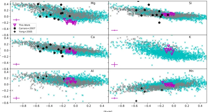
To compare with our results (see Figure 6), we have assembled (1) a sample of dwarf stars in the solar neighborhood from Bensby et al. (2014) (gray crosses in Mg, Ca, Si and Al panels); (2) a sample of dwarf stars in the solar neighborhood from Battistini & Bensby (2015) (gray crosses in the Mn panel); (3) a sample of F and G main-sequence stars of the disk taken from Chen et al.(2000) (gray crosses in the K panel); (4) a sample of cluster and ﬁeld red giants and a small fraction of dwarf stars from APOGEE-Kepler Asteroseismology Collaboration (henceforth, APO-KASC sample), which were re-analyzed using BACCHUS by Hawkins et al.(2016) (cyan crosses in Mg, Si, Ca, K, Al and Mn panels); and (5) Galactic anti-center OCs from Carraro et al. (2007) and Yong et al. (2005) (black stars and black pluses, respectively). Finally, we show our results using FERRE/MARCS stellar parameters, which are represented with magenta triangles.

1. α-elements: Magnesium, silicon, and calcium are gen-erally considered asα-elements, because they are formed by fusion involving α-particles. These elements can be produced in large quantities by SNe II(Samland1998). [α/Fe] decreases while metallicity increases after the onset of SNe Ia (e.g., Bensby et al. 2014and Hawkins et al.2016). If we look closely, this trend is separated into two sequences, especially for Mg. Using the APOGEE data, Hayden et al.(2015) found that the higher [α/Fe], more metal-poor sequence is dominated by thick-disk stars, while the lower[α/Fe], more metal-rich sequence is dominated by thin-disk stars. In general, our results follow the pattern formed by(thin disk) ﬁeld stars at the metallicity of IC 166 members, except for Mg. However, similar to Hawkins et al. (2016), the magnesium abundances that we have found from our manual analysis are lower compared to Bensby et al.(2014), though they still agree within the uncertainties.

Galactic anti-center OCs from Carraro et al.(2007) form trends of[α/Fe]−[Fe/H] very similar to the field stars: [α/Fe] decreases as [Fe/H] increases. It also appears that the scatter of [Mg/Fe] is larger than that of [Si/Fe] and [Ca/Fe], which also closely resembles field stars. IC 166 is one of the Galactic anti-center OCs with relatively high metallicity. Its α-element abun-dances generally fit in the trends defined by other Galactic anti-center OCs, though with slightly lower Mg abundances.

2. Light odd-Z elements: Potassium is primarily the result of oxygen burning in massive stellar explosions (Clayton 2007), so it is related to α-element formation (Zhang et al. 2006), expelled from SNe II (Samland 1998). Although there is not much observational data for K, the available data indicate that its abundance increases as metallicity decreases. Figure6shows that the results from Chen et al.(2000) are shifted to higher abundances with respect to that of Hawkins et al.(2016), probably due to differences in the adopted solar abundances.

Our results follow the expected trend forﬁeld stars at this metallicity.

Table 4

Estimated Uncertainties on Abundances Due to Stellar Parameter Uncertainties Element ΔTeff Δlog(g) Δ[Fe/H] Δξ σ

(+50 K) (+0.20dex) (+0.20 dex) (+0.20 km s−1) Mg +0.06 −0.09 +0.01 −0.02 0.11 Si +0.03 −0.05 +0.02 −0.03 0.07 Ca +0.05 −0.02 −0.04 −0.02 0.07 Al +0.05 −0.07 +0.00 −0.02 0.09 K +0.06 −0.01 −0.15 −0.01 0.16 Mn +0.03 −0.01 −0.04 −0.02 0.05 Fe +0.05 −0.02 +0.02 −0.03 0.06

(8)

Aluminum is formed during carbon burning in massive stars, mostly by the reactions between26Mg and excess neutrons (Clayton 2007). The Al abundances may also be changed through the Mg–Al cycle at extremely high temperature, e.g., inside AGB stars (Samland 1998; Arnould et al.1999). Literature values indicate that the Al abundance decreases as metallicity increases, and it stays relatively constant for metallicity greater than solar. The large dispersion found in the ASPCAP Al abundance results for IC 166 are not found in the literature for any OC, nor in our manual results. As discussed above, this is due to problems in the ASPCAP analysis. Four Galactic anti-center OCs from Yong et al.(2005), together with IC 166 form a similar [Al/Fe]−[Fe/H] trend as ﬁeld stars.

3. Iron-peak elements: Manganese is thought to form in explosive silicon burning (Woosley & Weaver 1995; Clayton 2007; Battistini & Bensby 2015). Significant amounts of manganese are produced by both SN type II and SN type Ia (Clayton 2007). According to the observations, Mn closely follows Fe. Our results for Mn fall within the abundance distribution outlined by field stars at similar metallicity. Three Galactic anti-center OCs from Yong et al.(2005), together with IC 166 form a similar [Mn/Fe]−[Fe/H] trend as field stars. An excep-tion is found for Be 31, where Yong et al. (2005) suggested observations of additional members of Be 31 are required to confirm low [Mn/Fe] in all Be 31 cluster members.

To summarize, the results obtained in this study (using the BACCHUS code) are in good agreement with literature results about ﬁeld giant/dwarf stars. The chemical abundances also verify that IC 166 is a typical anti-Galactic center OC, with relatively high metallicity among the others.

4.4. OC Metallicity Trend Around RGCof IC 166

Studies of the Galactic radial metallicity gradient(Friel1995; Frinchaboy et al. 2013; Cunha et al. 2016; Jacobson et al. 2016) are critical to understand the chemical evolution of the Galactic disk. Open clusters are one of the best tracers for this purpose, because they are located along the whole Galactic disk and they provide relatively easily measured chemical and kinematic properties. Most works agree that the metallicity decreases with increasing Galactic radius, at least for older OCs. However, the exact value of the metallicity gradient slope is still unclear(Cunha et al.2016; Jacobson et al.2016), as is the location of a possible break in the metallicity trend(Yong et al.2012; Reddy et al.2016).

In this work, we analyze the high-resolution spectra of IC 166 stars, and derive a metallicity of[Fe/H]=−0.08±0.05 dex. Since IC 166 (RGC≈12.7 kpc) is located near the possible

transition zone around RGC≈10–13 kpc (Yong et al. 2012;

Frinchaboy et al. 2013; Reddy et al. 2016), it may be enlightening to compare our results to the other high-resolution chemical abundance analysis on OCs near this region. For example, at RGC≈10.5 kpc, Sales Silva et al. (2016) derived a

metallicity of−0.02±0.05 dex for Tombaugh 1; Souto et al. (2016) reported a metallicity of −0.16±0.04 dex for NGC 2420 at RGC≈11 kpc. More strikingly, Reddy et al. (2016)

showed that the metallicities of OCs between 10 and 13 kpc (including about 15 OCs) vary between 0 and −0.4 (their Figure 4). They suggested this region is the transition zone between thin-disk OCs and thick-disk OCs. Therefore, IC 166, Tombaugh 1, and NGC 2420 safelyﬁt in the metallicity range deﬁned by other OCs in this region. A discussion about the existence of this break requires a large number of OCs at different RGC, which is certainly beyond the scope of this single

OC concentrated work. Readers are referred to Yong et al. (2012), Reddy et al. (2016) for discussion about this topic.

Figure 6.IC 166 results are compared with the literature, cyan crosses for Hawkins et al.(2016) results, while gray crosses for Ca, Mg, Si, and Al abundances from

Bensby et al.(2014). The sources of the gray crosses for K and Mn are Chen et al. (2000) and Battistini & Bensby (2015), respectively. The Galactic anti-center OCs

(9)

4.5. [ Fea ] versus [Fe/H]

As noted above,α-elements are formed from reactions with α-particles (He nuclei), which are active in SNe II. On the other hand, Fe is generated in SN Ia (although also, in smaller amounts, in SNe II); therefore, [α/Fe] is related to the ratio of Type II over Type Ia SNe that have enriched a particular star-forming environment.

Because the main polluters of the ISM in the early stages of galaxy formation are SNe II, we see enhanced α-element abundances at low metallicities. After∼1 Gyr, SNe Ia start to explode, generating a signiﬁcant amount of iron-peak elements but insigniﬁcant amounts of α-elements, and the iron-peak element fraction in the ISM increases quickly (Bensby et al.2005); [α/Fe] decreases as the metallicity increases.

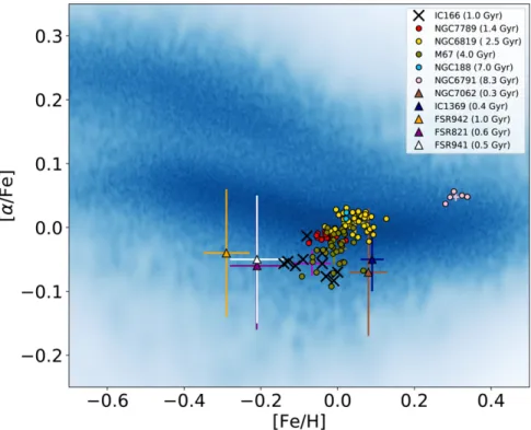
Figure 7 shows stars from APOGEE DR14 as gray dots. Results from ASPCAP DR13 forﬁve OCs (M67, NGC 7789, NGC 6819, NGC 6791, and NGC 188 in green, red, yellow, blue, and pink dots, respectively) studied by Linden et al. (2017) are added, and also the results from this study for IC 166(purple dots). The α-elements in this plot are an average of the elements Mg, Si, and Ca. All of the IC 166 stars are close to the expected trend for thin-disk stars (with a mean [α/Fe]∼ −0.05), although our abundance results are slightly more scattered when compared to the results for the other clusters.

IC 166 falls within the region of lowα-sequence. Thus, the chemical signatures of IC 166 appear to follow the same abundance trends as thin-disk ﬁeld stars (see Figure 7); very similar to other know disk OCs like NGC 7062, IC 1369, FSR 942, FSR 821, and FSR 941 studied in Frinchaboy et al. (2013).

5. The Orbit of IC 166

In order to estimate for the ﬁrst time a probable Galactic orbit for IC 166, the positional information of IC 166,

, 01 46 , 61 23

J2000 J2000 h m

a d =  ¢

( ) , was combined with the

newly measured proper motions and parallaxes from Gaia DR2(Gaia Collaboration et al.2018; Lindegren et al.2018) as well as with the existing line-of-sight velocities from the APOGEE survey. There were 13 stars in our sample, which were in the Gaia DR2 catalog and had a good parallax signal-to-noise (p p >w 3; see Table 5). For the 13 members surveyed by APOGEE (for which the membership is most certain), we estimate the mean proper motion of IC 166 as (μα,μδ)=(−1.429 ± 0.083, 1.139 ± 0.075) mas yr−1, a RV of

−40.58±1.59 km s−1_{, and a median parallax,} _{( p}_{á ñ }_s

p)=

(0.18466±0.05095), distance of 5.415±1.494 kpc, our distance estimated from parallax tend to agree with the mean distance estimated from a Bayesian approach using priors based on an assumed density distribution of the MW (e.g., Bailer-Jones et al. 2018), 4.485±0.89 kpc. It is important to note that our assumed Monte Carlo approach to compute the orbital elements are similar, adopting both distance estimates and therefore do not affect the results presented in this work.

For the Galactic model, we employ the Galactic dynamic software GravPot1626(J. G. Fernández-Trincado et al. 2018, in preparation), a semi-analytic, steady-state, three-dimensional gravitational potential based on the mass density distributions of the Besançon Galactic model (Robin et al.2003,2012,2014), observationally and dynamically constrained. The model is constituted by seven thin-disk components, two thick disks, an

Figure 7.Density map for[α/Fe] vs. [Fe/H], illustrating the high and low α-sequence formed by thick- and thin-disk stars observed by APOGEE DR14. Five open clusters studied by Linden et al.(2017) (M67, NGC 7789, NGC 6819, NGC6791, and NGC 188 in green, red, yellow, pink, and cyan dots, respectively) are also

shown. A sample ofﬁve new OCs (NGC 7062, IC 1369, FSR 942, FSR 821, and FSR 941 in brown, blue, orange, purple, and white triangles, respectively) studied by Frinchaboy et al.(2013) poorly alpha-enriched. Stars of IC 166 are shown as black “x” symbols. The colored crosses show the mean abundances and the standard

deviation for each cluster.

26

(10)

interstellar medium(ISM), a Hernquist stellar halo, a rotating bar component, and is surrounded by a spherical dark matter halo component that ﬁts fairly well the structural and dynamical parameters of the MW to the best we know them. A description of this model and its updated parameters appears in a score of papers (Fernández-Trincado et al.2016,2017a,2017b,2017c; Tang et al.2017,2018; Libralato et al.2018).

The Galactic potential is scaled to the Sun’s galactocentric distance, 8.3±0.23 kpc, and the local rotation velocity, 239±7 km s−1 (e.g., Brunthaler et al. 2011). We assumed the Sun’s orbital velocity vector [U_e, V_e, W_e]=[11.1 0.75

0.69 -+ , 12.24 0.47 0.47 -+ _{, 7.25} 0.36 0.37 -+

] (Schönrich et al. 2010). A long list of studies in the literature has presented different ranges for the bar pattern speeds. For our computations, the valuesΩbar=35,

40, 45, and 50 km s−1 kpc−1 are employed. These values are consistent with the recent estimate ofΩbargiven by

Fernández-Trincado et al. 2017b; Monari et al. 2017a, 2017b; Portail et al.2017. We consider an angle off=20° for the present-day orientation of the major axis of the Galactic bar and the Sun–Galactic center line. The total mass of the bar taken in this work is 1.1×1010 M_e, which corresponds to the dynamical constraints towards the MW bulge from massless particle simulations(Fernández-Trincado et al.2017b) and is consistent with the recent estimate given by Portail et al. (2017).

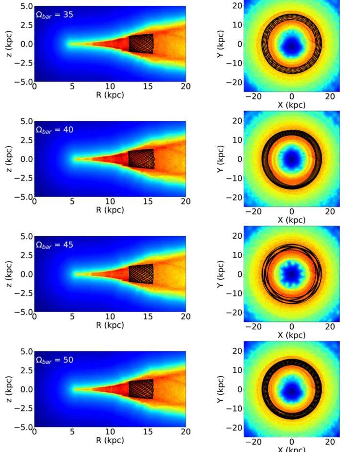
The probable orbit of IC 166 is computed adopting a simple Monte Carlo procedure for different bar pattern speeds as mentioned above. For each of 103 simulations, we time-integrated backwards the orbits for 2.5 Gyr under variations of the initial conditions (proper motions, RV, heliocentric distance, solar position, solar motion, and the velocity of the local standard of rest) according to their estimated errors, where the errors are assumed to follow a Gaussian distribution. The results of these computations are shown in Figure 8. The same ﬁgures display the probability densities of the resulting orbits projected on the meridional and equatorial Galactic planes in the non-inertial reference frame where the bar is at rest. The yellow and red colors correspond to more probable regions of the space, which are crossed more frequently by the simulated orbits. The ﬁnal point of each of these orbits has a very similar position to the current one of IC 166.

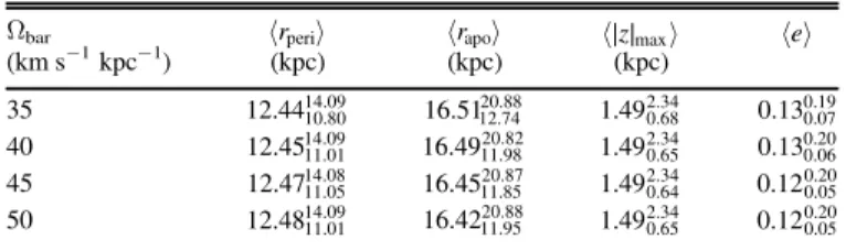
The median values of the orbital elements for the 103 realizations are listed in Table 6. Uncertainties in the orbital

integrations are estimated as the 16th (lower limit) and 84th (upper limit) percentile values. We deﬁned the orbital eccentricity as e r r r r , apo peri apo peri = -+ ( ) ( )

where rapois the apogalactic distance and rperithe perigalactic

distance. Weﬁnd the orbit of IC 166 lies in the Galactic disk and it appears to be an unremarkable typical Galactic OC.

6. Conclusions

We have presented the first high-resolution spectroscopic observations of the stellar cluster IC 166, which was recently surveyed in the H-band of APOGEE. Based on their sky distribution, RV, metallicity, CMD position, and proper motions, we have identified the 13 highest likelihood cluster members. We derived, for the first time, manual abundance determinations for up to eight chemical species (Mg, Ca, Ti, Si, Al, K, Fe, and Mn). High-resolution spectra are consistent with the cluster having a metallicity of [Fe/H]=−0.08± 0.05 dex. Isochrone fits indicate that the cluster is about 1.0±0.2 Gyr in age.

The results presented here show the cluster lies in the low-α sequence near the solar neighborhood, i.e., the cluster lies in the locus dominated by the low-α sequence of the canonical thin disk. We also found excellent agreement between our chemical abundances and general Galactic trends from large-scale studies.

It is important to note that our manual analysis was able to reduce the dispersion found by APOGEE/ASPCAP pipeline for most of the chemical species studied in this work. The most notable improvement was for[Al/Fe] abundance ratios.

Lastly, numerical integration of the possible orbits of IC 166 shows that the cluster appears to be an unremarkable standard Galactic OC with an orbit bound to the Galactic plane. The maximum and minimum Galactic distance achieved by the cluster as well as its orbital eccentricity suggest star formation at large Galactocentric radii. These results suggest that IC 166 could have formed nearer the solar neighborhood, fully compatible with the majority of known Galactic OCs at similar

(11)

metallicity. However, the derived orbital eccentricity (∼0.13) of the cluster is found be compatible with thin-disk popula-tions, but the maximum height above the plane, Zmax, larger than 1.5 kpc like IC 166 is too high for the thin disk and more compatible with the thick disk. It is important to note that, because the orbital excursions in our simulations are in the external part of the Galaxy (up to 16.5 kpc), it is in a region where the disk of the MW is known to exhibit a signiﬁcant ﬂare (e.g., Reylé et al.2009) and warp (Momany et al.2006; Carraro et al.2007). Such dynamical behavior has also been observed in anti-center old OCs, like Gaia 1(e.g., Koposov et al.2017; Carraro2018; Koch et al.2018).

We further note some important limitations of our orbital calculations: we ignore secular changes in the MW potential over time. We also ignore the fact that the MW disk exhibits a prominent warp andﬂare in the direction of IC 166. The MW potential that we used in the simulations is made up of the seven time-independent thin disks (Robin et al. 2003) with Einasto laws (Einasto1979).

We would like to thank John Donor for helpful comments in the manuscript. We are grateful to the referee for a prompt and constructive report. J.G.F.-T. is supported by FONDECYT No. 3180210. J.S.-U. and D.G. gratefully acknowledge support from the Chilean BASAL Centro de Excelencia en Astrofísica y Tecnologías Aﬁnes (CATA) grant PFB-06/2007. B.T. acknowledges support from the one-hundred-talent project of Sun Yat-Sen University. S.V. gratefully acknowledges the support provided by Fondecyt reg n. 1170518. D.M. is supported by the BASAL Center for Astrophysics and Associated Technologies (CATA) through grant PFB-06, by the Ministry for the Economy, Development and Tourism, Programa Iniciativa Cientíﬁca Milenio grant IC120009, awarded to the Millennium Institute of Astrophysics (MAS), and by FONDECYT Regular grant No. 1170121. Sz.M. has been supported by the Premium Postdoctoral Research Program of the Hungarian Academy of Sciences, and by the Hungarian NKFI Grants K-119517 of the Hungarian National

Research, Development and Innovation Ofﬁce. P.M.F. acknowledges support by an National Science Foundation AAG grants AST-1311835 & AST-1715662. V.V.S. and K.C. acknowledge support from NASA grant NNX17AB64G. O.Z., F.D., T.M., and D.A.G.H. acknowledge support provided by the Spanish Ministry of Economy and Competitiveness (MINECO) under grant AYA-2014-58082-P.

Funding for the GravPot16 software has been provided by the Centre national d’études spatiales (CNES) through grant 0101973 and UTINAM Institute of the Université de Franche-Comté supported by the Région de Franche-Franche-Comté and Institut des Sciences de l’Univers (INSU). Simulations have been executed on computers from the Utinam Institute of the Université de Franche-Comté supported by the Région de Franche-Comté and Institut des Sciences de l’Univers (INSU), and on the supercomputer facilities of the Mésocentre de calcul de Franche-Comté.

Funding for the Sloan Digital Sky Survey IV(SDSS-IV) has been provided by the Alfred P. Sloan Foundation, the US Department of Energy Ofﬁce of Science, and the Participating Institutions. SDSS-IV acknowledges support and resources from the Center for High-Performance Computing at the University of Utah. The SDSS website ishttp://www.sdss.org. SDSS-IV is managed by the Astrophysical Research Consortium for the Participating Institutions of the SDSS Collaboration including the Brazilian Participation Group, the Carnegie Institution for Science, Carnegie Mellon University, the Chilean Participation Group, the French Participation Group, Harvard-Smithsonian Center for Astrophysics, Instituto de Astrofísica de Canarias, The Johns Hopkins University, Kavli Institute for the Physics and Mathematics of the Universe (IPMU)/University of Tokyo, Lawrence Berkeley National Laboratory, Leibniz Institut für Astrophysik Potsdam (AIP), Max-Planck-Institut für Astronomie (MPIA Heidelberg), Max-Planck-Institut für Astrophysik (MPA Garching), Max-Planck-Institut für Extraterrestrische Physik (MPE), National Astronomical Observatory of China, New Mexico State University, New York University, University of Notre Dame, Observatorio Nacional/MCTI, The Ohio State University, Pennsylvania State University, Shanghai Astronomical Obser-vatory, United Kingdom Participation Group, Universidad Nacional Autónoma de México, University of Arizona, University of Colorado Boulder, University of Oxford, University of Portsmouth, University of Utah, University of Virginia, University of Washington, University of Wisconsin, Vanderbilt University, and Yale University.

Appendix A

Elemental Abundances Line-by-line

Table7shows the individual abundances measured for each atomic lines analyzed of Mg, Ca, Si, K, Ti, Al, Mn, and Fe.

Table 6

Orbital Elements of IC 166 Estimated with the Newly Measured Proper Motions and Parallax from Gaia DR2 Data Combined with Existing

Line-of-sight Velocities from APOGEE

Ωbar árperiñ árapoñ á∣ ∣zmaxñ á ñe (km s−1_kpc−1₎ _(kpc) _(kpc) _(kpc) 35 12.44_10.8014.09 _16.51 12.7420.88 1.490.682.34 0.130.070.19 40 12.4511.0114.09 16.4911.9820.82 1.490.652.34 0.130.060.20 45 12.4711.0514.08 16.4511.8520.87 1.490.642.34 0.120.050.20 50 12.48_11.0114.09 _16.42 11.9520.88 1.490.652.34 0.120.050.20 Note.The average value of the orbital parameters of IC 166 was found for 106

realizations adopting a Monte Carlo approach, with uncertainty ranges given by the 16th(subscript) and 84th (superscript) percentile values.

(12)

A Mg á ( )ñ 7.26±0.01 7.27±0.03 7.28±0.02 7.26±0.04 7.30±0.02 7.31±0.03 7.29±0.07 7.17±0.03 7.18±0.04 7.35±0.04 7.26±0.11 7.32±0.06 7.22±0.04 [Mg/Fe] −0.16±0.01 −0.25±0.03 −0.16±0.02 −0.23±0.04 −0.19±0.02 −0.19±0.03 −0.17±0.07 −0.23±0.03 −0.22±0.04 −0.18±0.04 −0.10±0.11 −0.13±0.06 −0.17±0.04 Ca 16136.80 ... 6.07 6.04 6.17 6.14 6.09 ... ... ... ... ... ... ... 16150.80 6.05 6.29 6.30 6.17 6.26 6.28 ... ... 6.04 6.28 ... 6.18 6.11 16157.40 6.13 ... ... 6.25 6.29 ... ... ... 6.30 6.18 ... ... ... 16197.10 6.25 6.29 ... 6.34 6.31 ... ... ... ... ... ... 6.36 ... A Ca á ( )ñ 6.14±0.10 6.22±0.13 6.17±0.18 6.23±0.08 6.25±0.08 6.18±0.13 ... ... 6.17±0.18 6.23±0.07 ... 6.27±0.13 6.11 [Ca/Fe] −0.06±0.10 −0.08±0.13 −0.05±0.18 −0.04±0.08 −0.02±0.08 −0.10±0.13 ... ... −0.01±0.18 −0.08±0.07 ... 0.04±0.13 −0.06 K 15163.10 4.85 5.01 5.08 ... 5.12 ... 5.02 ... ... ... ... ... ... 15168.40 4.99 5.08 4.97 ... 5.15 4.93 ... 4.98 ... ... ... 5.14 ... A K á ( )ñ 4.92±0.10 5.04±0.05 5.02±0.08 ... 5.13±0.02 4.93 5.02 4.98 ... ... ... 5.14 ... [K/Fe] −0.05±0.10 −0.03±0.05 0.03±0.08 ... 0.04±0.02 −0.12 0.01 0.03 ... ... ... 0.14 ... Si 15376.80 7.32 7.46 ... ... 7.45 7.59 ... 7.40 ... ... ... 7.46 ... 15557.80 7.42 7.63 7.39 7.58 7.54 7.59 7.39 7.42 ... 7.55 ... 7.27 7.36 15884.50 7.29 7.45 ... 7.32 7.44 7.40 7.33 7.29 7.33 7.38 7.21 7.31 7.19 15960.10 7.64 7.73 7.55 7.54 7.73 7.59 7.59 ... 7.55 7.59 7.38 7.88 7.55 16060.00 ... ... ... 7.79 ... ... ... 7.45 ... ... 7.66 7.53 7.52 16094.80 ... 7.58 7.53 ... 7.52 7.43 7.43 ... 7.50 7.54 ... 7.61 7.45 16215.70 ... 7.71 ... 7.55 7.64 7.73 ... ... 7.49 7.74 7.55 ... ... 16241.80 ... 7.71 ... 7.64 ... ... 7.56 7.49 7.56 ... 7.51 7.36 ... 16680.80 7.51 7.38 7.45 ... 7.61 7.45 7.51 7.41 7.39 7.57 7.42 7.42 7.51 16828.20 ... ... ... ... ... ... ... 7.55 7.37 ... ... ... ... A Si á ( )ñ 7.44±0.14 7.58±0.14 7.48±0.07 7.57±0.15 7.56±0.10 7.54±0.12 7.48±0.10 7.43±0.08 7.45±0.09 7.56±0.11 7.41±0.13 7.48±0.20 7.43±0.13 [Si/Fe] 0.04±0.14 0.08±0.14 0.06±0.07 0.10±0.15 0.09±0.10 0.06±0.12 0.04±0.10 0.05±0.08 0.07±0.09 0.05±0.11 0.07±0.13 0.05±0.20 0.06±0.13 Ti 15715.60 4.71 4.78 ... ... ... ... ... ... ... 4.84 ... ... 4.78 A Ti á ( )ñ 4.71 4.78 ... ... ... ... ... ... ... 4.84 ... ... 4.78 [Ti/Fe] −0.08 −0.11 ... ... ... ... ... ... ... −0.06 ... ... 0.02 Mn 15159.20 5.26 5.28 ... 5.28 ... 5.34 ... 5.26 ... 5.34 ... 5.31 ... 15217.70 5.23 5.38 5.37 5.25 5.37 5.32 5.31 5.23 5.19 5.34 5.27 ... ... 15262.40 ... 5.29 5.20 5.37 ... ... 5.25 5.29 5.32 5.35 5.30 5.33 ... 11 Schiappacasse-Ulloa et al.

(13)

Table 7 (Continued) Element

air

l star1 star2 star3 star4 star5 star6 star7 star8 star9 star10 star11 star12 star13

A Mn á ( )ñ 5.24±0.02 5.32±0.05 5.28±0.12 5.30±0.06 5.37 5.33±0.01 5.28±0.04 5.26±0.03 5.25±0.09 5.34±0.01 5.28±0.02 5.32±0.01 ... [Mn/Fe] −0.04±0.02 −0.06±0.05 −0.02±0.12 −0.05±0.06 0.02 −0.03±0.01 −0.04±0.04 0.00±0.03 −0.01±0.09 −0.05±0.01 0.06±0.02 0.01±0.01 ... Al 16719.00 6.51 6.45 6.47 6.47 ... ... 6.43 6.38 6.45 6.51 ... 6.39 ... 16750.60 6.37 6.41 6.45 6.37 6.50 6.48 6.32 6.18 6.36 6.39 6.33 6.37 ... A Al á ( )ñ 6.44±0.10 6.43±0.03 6.46±0.01 6.42±0.07 6.50 6.48 6.37±0.08 6.28±0.14 6.40±0.06 6.45±0.08 6.33 6.38±0.01 ... [Al/Fe] 0.18±0.10 0.07±0.03 0.18±0.01 0.09±0.07 0.17 0.14 0.07±0.08 0.04±0.14 0.16±0.06 0.07±0.08 0.13 0.08±0.01 ... 12 Astronomical Journal, 156:94 (14pp ), 2018 September Schiappacasse-Ulloa et al.

(14)

Figure 8. Probability density maps color-coded at the bottom for the meridional orbits in the R z, plane(column 1) and face-on (column 2) of 1000 random realizations of IC 166 time-integrated backwards for 2.5 Gyr adopting the newly measured proper motions and parallax from Gaia DR2 (Gaia Collaboration et al.2018; Lindegren et al.2018) . Red and yellow colors correspond to larger probabilities. The tile size of the HealPix map is 0.10 kpc2. The black line shows the orbit using the best values found for the cluster(see the text).

(15)

Appendix B

Orbit of IC 166 with Monte Carlo Calculations Figure8 shows the Monte Carlo simulations for the bound orbit of IC 166. We make these Monte Carlo simulations to estimate the uncertainties in the orbital elements(see the text).

ORCID iDs J. Schiappacasse-Ulloa https: //orcid.org/0000-0002-2179-9363 D. Geisler https://orcid.org/0000-0002-3900-8208 P. Frinchaboy https://orcid.org/0000-0002-0740-8346 M. Schultheis https://orcid.org/0000-0002-6590-1657 S. Villanova https://orcid.org/0000-0001-6205-1493 D. Souto https://orcid.org/0000-0002-7883-5425 K. Vieira https://orcid.org/0000-0001-5598-8720 D. Minniti https://orcid.org/0000-0002-7064-099X G. Zasowski https://orcid.org/0000-0001-6761-9359 A. Pérez-Villegas https://orcid.org/0000-0002-5974-3998 F. A. Santana https://orcid.org/0000-0002-4023-7649 R. Carrera https://orcid.org/0000-0001-6143-8151 A. Roman-Lopes https://orcid.org/0000-0002-1379-4204 References

Abolfathi, B., Aguado, D. S., Aguilar, G., et al. 2018,ApJS,235, 42

Allende Prieto, C., Beers, T. C., Wilhelm, R., et al. 2006,ApJ,636, 804

Arnould, M., Goriely, S., & Jorissen, A. 1999, A&A,347, 572

Asplund, M., Grevesse, N., & Sauval, A. J. 2005, in ASP Conf. Ser. 336, Cosmic Abundances as Records of Stellar Evolution and Nucleosynthesis, ed. T. G. Barnes, III & F. N. Bash(San Francisco, CA: ASP),25

Bailer-Jones, C. A. L., Rybizki, J., Fouesneau, M., Mantelet, G., & Andrae, R. 2018, arXiv:1804.10121

Battistini, C., & Bensby, T. 2015,A&A,577, A9

Bensby, T., Feltzing, S., Lundström, I., & Ilyin, I. 2005,A&A,433, 185

Bensby, T., Feltzing, S., & Oey, M. S. 2014,A&A,562, A71

Blanton, M. R., Bershady, M. A., Abolfathi, B., et al. 2017,AJ,154, 28

Bonatto, C., Kerber, L. O., Bica, E., & Santiago, B. X. 2006,A&A,446, 121

Bressan, A., Marigo, P., Girardi, L., et al. 2012,MNRAS,427, 127

Brunthaler, A., Reid, M. J., Menten, K. M., et al. 2011,AN,332, 461

Burkhead, M. S. 1969,AJ,74, 1171

Carraro, G. 2018,RNAAS,2, 12

Carraro, G., & Chiosi, C. 1994, A&A,287, 761

Carraro, G., Geisler, D., Villanova, S., Frinchaboy, P. M., & Majewski, S. R. 2007,A&A,476, 217

Carraro, G., Ng, Y. K., & Portinari, L. 1998,MNRAS,296, 1045

Chen, Y. Q., Nissen, P. E., Zhao, G., Zhang, H. W., & Benoni, T. 2000,

A&AS,141, 491

Clayton, D. 2007, Handbook of Isotopes in the Cosmos (Cambridge: Cambridge Univ. Press)

Cunha, K., Frinchaboy, P. M., Souto, D., et al. 2016,AN,337, 922

Cunha, K., Smith, V. V., Hasselquist, S., et al. 2017,ApJ,844, 145

de la Fuente Marcos, R., & de la Fuente Marcos, C. 2004,NewA,9, 475

Deng, L., & Xin, Y. 2007, in ASP Conf. Ser. 374, From Stars to Galaxies: Building the Pieces to Build Up the Universe, ed. A. Vallenari et al.(San Francisco, CA: ASP),387

De Silva, G. M., Freeman, K. C., Bland-Hawthorn, J., et al. 2015,MNRAS,

449, 2604

Dias, W. S., Alessi, B. S., Moitinho, A., & Lépine, J. R. D. 2002,A&A,389, 871

Dias, W. S., Monteiro, H., Caetano, T. C., et al. 2014,A&A,564, A79

Donati, P., Cantat Gaudin, T., Bragaglia, A., et al. 2014,A&A,561, A94

Einasto, J. 1979, in IAU Symp. 84, The Large-Scale Characteristics of the Galaxy, ed. W. B. Burton(Dordrecht: Reidel),451

Fernández-Trincado, J. G., Geisler, D., Moreno, E., et al. 2017a, in SF2A-2017, Proc. Annual meeting of the French Society of Astronomy and Astrophysics, ed. C. Reylé et al.,199

Fernández-Trincado, J. G., Robin, A. C., Moreno, E., et al. 2016, ApJ,

833, 132

Fernández-Trincado, J. G., Robin, A. C., Moreno, E., Pérez-Villegas, A., & Pichardo, B. 2017b, in SF2A-2017, Proc. Annual meeting of the French Society of Astronomy and Astrophysics, ed. C. Reylé et al.,193

Fernández-Trincado, J. G., Zamora, O., García-Hernández, D. A., et al. 2017c,

ApJL,846, L2

Fernández-Trincado, J. G., Zamora, O., Souto, D., et al. 2018, arXiv:1801.07136

Friel, E. D. 1995,ARA&A,33, 381

Friel, E. D. 2013, in Planets, Stars and Stellar Systems Vol. 5, ed. T. D. Oswalt & G. Gilmore(Dordrecht: Springer Science+Business Media),347

Friel, E. D., Donati, P., Bragaglia, A., et al. 2014,A&A,563, A117

Friel, E. D., & Janes, K. A. 1993, A&A,267, 75

Friel, E. D., Liu, T., & Janes, K. A. 1989,PASP,101, 1105

Frinchaboy, P. M., Thompson, B., Jackson, K. M., et al. 2013,ApJL,777, L1

Gaia Collaboration, Brown, A. G. A., Vallenari, A., et al. 2018, arXiv:1804.09365

García Pérez, A. E., Allende Prieto, C., Holtzman, J. A., et al. 2016,AJ,151, 144

Geisler, D., Claria, J. J., & Minniti, D. 1997,PASP,109, 799

Gieles, M., Portegies Zwart, S. F., Baumgardt, H., et al. 2006,MNRAS,371, 793

Gieles, M., & Renaud, F. 2016,MNRAS,463, L103

Gilmore, G., Randich, S., Asplund, M., et al. 2012, Msngr,147, 25

Gunn, J. E., Siegmund, W. A., Mannery, E. J., et al. 2006,AJ,131, 2332

Gustafsson, B., Edvardsson, B., Eriksson, K., et al. 2008,A&A,486, 951

Hasselquist, S., Shetrone, M., Cunha, K., et al. 2016,ApJ,833, 81

Hawkins, K., Masseron, T., Jofré, P., et al. 2016,A&A,594, A43

Hayden, M. R., Bovy, J., Holtzman, J. A., et al. 2015,ApJ,808, 132

Jacobson, H. R., Friel, E. D., Jílková, L., et al. 2016,A&A,591, A37

Janes, K. A. 1979,ApJS,39, 135

Kharchenko, N. V., Piskunov, A. E., Schilbach, E., Röser, S., & Scholz, R.-D. 2012,A&A,543, A156

Koch, A., Hansen, T. T., & Kunder, A. 2018,A&A,609, A13

Koposov, S. E., Belokurov, V., & Torrealba, G. 2017,MNRAS,470, 2702

Lamers, H. J. G. L. M., & Gieles, M. 2006,A&A,455, L17

Lamers, H. J. G. L. M., Gieles, M., Bastian, N., et al. 2005,A&A,441, 117

Libralato, M., Bellini, A., Bedin, L. R., et al. 2018,ApJ,854, 45

Lindegren, L., Hernandez, J., Bombrun, A., et al. 2018, arXiv:1804.09366

Linden, S. T., Pryal, M., Hayes, C. R., et al. 2017,ApJ,842, 49

Liu, F., Yong, D., Asplund, M., Ramírez, I., & Meléndez, J. 2016,MNRAS,

457, 3934

Loktin, A. V., & Beshenov, G. V. 2003,ARep,47, 6

Magrini, L., Randich, S., Donati, P., et al. 2015,A&A,580, A85

Magrini, L., Sestito, P., Randich, S., & Galli, D. 2009,A&A,494, 95

Majewski, S. R., Schiavon, R. P., Frinchaboy, P. M., et al. 2017,AJ,154, 94

Masseron, T., Merle, T., & Hawkins, K. 2016, BACCHUS: Brussels Automatic Code for Characterizing High accUracy Spectra, Astrophysics Source Code Library, ascl:1605.004

Momany, Y., Zaggia, S., Gilmore, G., et al. 2006,A&A,451, 515

Monari, G., Famaey, B., Siebert, A., et al. 2017a,MNRAS,465, 1443

Monari, G., Kawata, D., Hunt, J. A. S., & Famaey, B. 2017b, MNRAS,

466, L113

Moyano Loyola, G. R. I., & Hurley, J. R. 2013,MNRAS,434, 2509

Portail, M., Gerhard, O., Wegg, C., & Ness, M. 2017,MNRAS,465, 1621

Randich, S., Gilmore, G. & Gaia-ESO Consortium 2013, Msngr,154, 47

Reddy, A. B. S., Lambert, D. L., & Giridhar, S. 2016,MNRAS,463, 4366

Reylé, C., Marshall, D. J., Robin, A. C., & Schultheis, M. 2009,A&A,495, 819

Robin, A. C., Marshall, D. J., Schultheis, M., & Reylé, C. 2012, A&A,

538, A106

Robin, A. C., Reylé, C., Derrière, S., & Picaud, S. 2003,A&A,409, 523