Eddy generation at a convex corner by a coastal current in a rotating system

EDDY GENERATION AT A CONVEX CORNER BY A

COASTAL CURRENT IN A ROTATING SYSTEM

by

Barry A. Klinger

S.B., Massachusetts Institute of Technology (1985)

Submitted in partial fulfillment of the requirements for the degree of DOCTOR OF PHILOSOPHY

at the

MASSACHUSETTS INSTITUTE OF TECHNOLOGY and the

WOODS HOLE OCEANOGRAPHIC INSTITUTION March 1992

@ Barry A. Klinger 1992

The author hereby grants to MIT and to WHOI permission to reproduce and to distribute copies of this thesis document in whole or in part.

Signature of Author ... s... ... ...

Joint Program in Physical Oceanography

Massachusetts Institute of Technology Woods Hole Oceanographic Institution

March 5, 1992 Certified by. John A. Whitehead Senior Scientist Thesis Supervisor Accepted by... ... .... ... '... . . . . . ... Lawrence J. Pratt Chairman, Joint Committee for Physical Oceanography Massachusetts Institute of Technology ds Hole Oceanographic Institution

Images in this thesis are of poor quality. This is the best copy available.

"While the solid appears in itself dead, moved only from without, the liquid and volatile make the impression of independent mobility and vitality..."

-quoted by Ved Mehta, The Stolen Light

Nur ein nar messt wasser.

[Only a fool measures water.]

EDDY GENERATION AT A CONVEX CORNER BY A COASTAL CURRENT IN A ROTATING SYSTEM

by

Barry A. Klinger

Submitted in partial fulfillment of the requirements for the degree of Doctor of Philosophy at the Massachusetts Institute of Technology

and the Woods Hole Oceanographic Institution March 5, 1992

Abstract

Rotating baroclinic and barotropic boundary currents flowing around a cor-ner in the laboratory were studied in order to discover the circumstances under which eddies were produced at the corner. Such flows are reminiscent of oceanic coastal flows around capes. When the baroclinic currents, which consisted of surface flows bounded by a density front, encountered a sharp corner, immediately downstream of the corner an anticyclone grew in the surface layer for an angle of greater than 40 degrees. Varying the initial condition of the flow or the depth of the lower layer did not noticeably affect the gyre's properties except for its growth speed, which was greater when the lower layer was shallower. The barotropic currents were pumped along a sloping bottom, and also formed anticyclonic gyres which quickly attained an approximately steady state. For a given topography, the size of the gyre was proportional to the inertial radius u/f. Volume flux calculations based on the sur-face velocity revealed vertical shear which increased with gyre size. Hydraulic models were also applied to flow around gently curving topography to determine the critical separation curvature as a function of upstream parameters.

Thesis Advisor: Dr. J. A. Whitehead

Table of Contents

Abstract ...

Acknowledgments ... 1. Introduction ...

1.1. Coasts, Currents, Capes, Channels, and Gyres . . . . . 1.2. Flow Separation in a Rotating and Non-rotating World 1.3. Previous Theoretical Studies . . . . 1.4. Plan of the Thesis . . . . 2. Hydraulic Models of Separation From Curved

2.1. Introduction . . . . 2.2. The System of Equations to be Solved . . . . . 2.3. Barotropic Flows Over a Flat Bottom . . . . . 2.4. Barotropic Flows Over a Sloping Bottom . . . . 2.5. Reduced Gravity Currents . . . . 2.6. Conclusions . . . . 3. Eddies Generated by a Density Front Current

in a Rotating Tank . . . . 3.1. Introduction . . . . 3.2. Apparatus and Procedure . . . . 3.3. Qualitative Behavior and Eddy Growth Rates 3.4. Interpolation of Fresh Water Velocity Fields . 3.5. Summary and Discussion . . . . Appendices to Chapter 3 . . . . 3.A. Technical Notes on Apparatus . . . . 3.B. Estimation of Interpolation Errors . . . .

Coastlines

at a Sharp Corner 74

77

86 102 113 121 121 125 . . .

4. Barotropic Sloping Bottom Flows Around a Corner in a Rotating

Tank ... ... 127

4.1. Introduction . . . . 127

4.2. Experimental Apparatus and Procedure . . . . 130

4.3. Qualitative Observations . . . . 138

4.4. Rossby Number and Gyre Size . . . . 143

4.5. Velocity, Transport, and Vorticity Profiles . . . . 156

4.6. Discussion and Conclusions . . . . 177

Appendix to Chapter 4 . . . . 181

4.A. Jitter Removal . . . . 181

5. Summary and Conclusions . . . . 184

R eferences . . . . 190

Acknowledgements

I would like to thank my advisor, Jack Whitehead, for many lessons in how one actually does science as well as for pushing me into deeper waters so I could swim by myself. Thanks go also to Glenn Flierl, my geophysical fluid dynamics guru and the man responsible for my entering physical oceanography graduate school in the first place, who contributed many ideas to this thesis and gave extensive computer and administrative support at MIT. The rest of my thesis committee-Larry Pratt, Nelson Hogg, and Phil Richardson-helped me refine and focus my thesis with their comments and discussion. Melvin Stern was not officially on my thesis committee, but our many scientific discussions were quite helpful to me. I could hardly have put together any experiments without the help of Robert Frazel, who has presided over the Geophysical Fluid Dynamics Lab since the dawn of time and has a knack for giving one some perspective on life in academia. The data analysis was based on work at the Motion Analysis facility at WHOI; the burden of its upkeep fell on the shoulders of Scott Gallager, who was kind enough to take time away from his own research to answer my numerous questions about the equipment. Roberta Young and Steve Meacham have been a great help in dealing with the computers at MIT. Anne Marie Michael saved me days of work by helping me with the mysteries of IATEX; much of this work was on her own time. Fellow Joint Program students-Dave Walsh, LuAnne Thompson, Sarah Gille, Changshen Chen, students-Dave Chester, Sarah

Green, Molly Baringer, Xiaoming Wang, Lorenzo Polvani, Keith Alverson, Gwyneth Hufford, and many others-have helped keep me sane while also keeping me on my toes with many clever comments and probing questions about my work.

I thank my parents, Linda and Rudy Klinger, and my sister, Elise Klinger, for their decades of faith in me, and my wife, Elise Berliner, whose love, help, and advice was like a ship carrying me over the storm-tossed seas of oceanography grad school.

This work was supported by the National Science Foundation grant OCE 89-15408.

Chapter 1.

Introduction

1.1.

Coasts, Currents, Capes, Channels, and Gyres

A dominant feature of the world's oceans is the ubiquity of eddies. Though the forcing of the general circulation is dominated by the basin-scale patterns of wind stress and surface heating and cooling, much of the energy of ocean currents resides in mesoscale structures, which have a spatial scale on the order of the local internal radius of deformation, and sub-mesoscale features. Since mesoscale eddies in the ocean are thought to be largely a consequence of baroclinic and barotropic instability of larger scale mean currents, much work on eddy generation has concentrated on the instability of geometrically simple currents, such as zonal or circular flows. However, it is also interesting to contemplate the dynamics of other mechanisms which may produce eddies. Laboratory and computer experiments as well as oceanic observations have shown that coastal currents that flow around a convex corner, such as a cape, are capable of generating eddies. In this thesis, we attempt to shed some light on the dynamics governing such eddy generation.

The Mediterranean Outflow is a prime example of a current flowing along a lateral boundary with a convex bend in it (see Figure 1.1.1). This current is a buoyancy-driven flow from the salty, warm Mediterranean to the relatively fresh and cold Atlantic (Ambar, Howe and Abdullah, 1976; Ambar and Howe, 1979a,b; Grundlingh, 1981; Howe, 1982; Madelain, 1970; Thorpe, 1976; Zenk, 1970, 1975, 1980). While the character of the dense plume is dominated by mixing and friction as it descends from the sill at Gibraltar along the continental shelf, by the time it reaches Cape Saint Vincent at the western end of the Gulf of Cadiz (Figure 1.1.1), it has attained a stable depth range marked by salinity and temperature maxima

centered at 1200 m and 800 m (Figure 1.1.2). As the Mediterranean water emerges from the Strait of Gibraltar, it rests completely on the sloping bottom, but by the time it reaches Cape Saint Vincent, the Outflow is bounded both above and below by Atlantic water, with the continental slope acting as a wall rather than a floor. Aver-age current speeds of 20-35 cm/s have been measured in the Mediterranean Outflow in the Gulf of Cadiz, with a current width on the order of 20 km for the flow filament closest to the shore and 60 km wide if we include other westward-flowing filaments (Figure 1.1.1).

Related to the Mediterranean Outflow are meddies, which are anticycloni-cally circulating subsurface lenses of water with water properties of the Outflow (Armi and Zenk, 1984; Kase and Zenk, 1987; Richardson et al., 1988). A typical meddy has a radius on the order of 50 km, maximum azimuthal current speeds of 20-25 cm/s,

and vertical property distributions as shown in Figure 1.1.3. While the maxima in property anomalies and rotation speed are clearly deep in the thermocline (as in the

Mediterranean Outflow, at about 1200 m), there is evidence that meddies do have a significant surface vorticity (Kase and Zenk, 1987).

The best studied meddies have all been observed on the order of 1000 km west of Cape Saint Vincent even though the meddy water characteristics are indicative of an origin near Cape Saint Vincent. Swallow (1969) reports a cyclone observed in the Gulf of Cadiz. His hydrography also showed a weak lens of salty water reminiscent of a meddy, but drifters placed in it showed no anticyclonic rotation. Sanford (1988, personal communication) reports an anticyclone observed forming off Cape Saint Vincent, but its 30 cm/s velocity maximum was only about 5 km from the center. Armi and Zenk (1984) estimate that it would take 20 days for the main branch and 10 days for the entire current to form a meddy. Richardson et al. (1988) estimate that 8 to 12 meddies are formed a year, implying that meddy formation must be happening at least a third of the time.

stations

Figure 1.1.2: Cross-shore profile of Mediterranean Outflow along line extending south from about

30 km south of Cape Saint Vincent (Ambar and Howe, 1979a, Figure 5). (a) Temperature, (b)

OXYGEN (y moles/kg) SALINITY 200 POTENTIAL. TEMP. (*C) 0 0 20

iOf

a 35 3 SALWY z wA '~ 2 SLICATEp -jums/k91 3 o 20 A 40 A GoC A SO A WI STATIONS 85-

104--Figure 1.1.3: Vertical profile of properties in a meddy and in a nearby "ambient" water station

85 km away (Armi and Zenk, 1984, Figure 1): potential temperature, salinity, oxygen, silicate, and a, vs. pressure, and potential temperature vs. salinity.

12

us

D'Asaro (1988) has hypothesized that meddies are generated by the Mediter-ranean Outflow at Cape Saint Vincent. He considered this an example of eddy genera-tion by a boundary current encountering a corner. Another example is the generagenera-tion of Beaufort Sea sub-mesoscale vortices by a surface coastal current flowing past Point Barrow on the northern coast of Alaska (Figure 1.1.4). There is better direct evidence of anticyclonic eddy formation at Point Barrow than there is at Cape Saint Vincent. For instance, in the summer of 1971 an occupied ice floe was carried along the coast by the current and after passing Point Barrow executed two anticyclonic loops with approximate radius of 5 km (about a Rossby radius) and approximate period of one day (Figure 1.1.5). Satellite infrared photography during the summer also shows sim-ilarly scaled cyclonic and anticyclonic features. In D'Asaro's conception, friction at the inshore edge of the coastal current generates a layer of negative vorticity, as in non-rotating flows, which is the source for the large negative relative vorticity of the anticyclonic eddies. Meddies have smaller negative relative vorticities, with rotation periods at the velocity maximum on the order of a week rather than a day.

There are other theories for the generation of meddies, such as McWilliams' (1985) proposal that they are formed by geostrophic adjustment as the plume descends from the Strait of Gibraltar. The most compelling of these explanations of meddy generation is the work of Kase and Zenk (1987) and Kase, Beckmann, and Hinricksen (1989). Their models suggest that meddies are broken off from the Mediterranean Outflow by stronger currents above the thermocline in the Atlantic off the coast of Portugal.

A situation which is similar to that of a coastal current flowing around a corner is that of the outflow from a strait which can form a gyre at the mouth of the strait. Such anticyclones have been observed in the Alboran Sea in the western Mediterranean (see Figure 1.1.6 and Lanoix, 1974) and in the outflow of the Tsugaru Sea in Japan (Conlon 1982; Kawasaki and Sugimoto, 1984). The Alboran gyre is fed

Figure 1.1.4: (a) Location and (b) topography of Barrow canyon and Point Barrow, suspected generation site of Beaufort Sea eddies (D'Asaro, 1988, Figure 1). Contours deeper than 1000 m are not shown.

Figure 1.1.5: Track of ice flow showing anticyclonic motion past Point Barrow, August 6-9, 1971, with heavy dots six hours apart (D'Asaro, 1988, Figure 4).

Figure 1.1.6: The Alboran gyre as seen in dynamic height map of western Mediterranean Sea

(Donde Va Group, 1984).

by the surface current which flows into the Mediterranean from the Strait of Gibraltar and detaches from a bend in the North African coast. The Tsugaru outflow is also a surface current, which has a seasonal change from a mode that remains attached to the coast and one that forms a gyre. Bormans (1988) reviews the literature on gyres produced by such flows. Numerical models of the Alboran gyre (Loth and Crepon, 1984; Preller, 1985; Werner et al., 1988) reproduced the gyre but did not isolate its cause.

The generation of eddies by a current flowing around a corner has been observed in several laboratory experiments in rotating systems.

Whitehead and Miller (1979) conducted a series of experiments in a rotating channel that opened at either end into a wider basin. The bends in the wall consisted of segments of circles. Initially a dam or gate was placed across the center of the channel, separating salty, dense water on one side from fresh, light water on the other (Figure 1.1.7). When the gate was removed, geostrophic adjustment created a current in each layer moving in opposite directions. The Rossby radius of deformation was varied from run to run, and the radius p of the circular bends in the walls took one of two values for each run. For a Rossby radius R small compared to the channel width

We, the currents had a width of about R and were concentrated close to the right

hand wall looking downstream. For R < We, the current was unstable, producing a

series of vortices of both signs, and for R > WC, the current veered right to stay near the wall as it emerged from the channel. For R > p the current outside the channel formed an anticyclone between the current and the wall near the channel opening. This eddy grew with time, but stayed attached to the wall. Figure 1.1.8 summarizes results.

Bormans and Garrett (1989) conducted similar experiments in which the fresh current flowed into water which had an ambient surface fresh layer. The relative depths of the two fresh layers controlled the Rossby number of the flow. For flows in

2r

I

r t 30 ern. I r t

Figure 1.1.7: Laboratory apparatus for experiments in which channel opened into wider basin and flow was initiated by geostrophic adjustment (Whitehead and Miller, 1979, Figure 3).

Figure 1.1.8: Representative flow regimes, channel flow into wider basin (Whitehead and Miller,

1979, Figure 4). Photos show surface currents flowing into dark region of tank, with each column a

different time sequence. From left to right, shows increasing Rossby radius runs: violently unstable flow, moderate instability, coastal trapped current, and single gyre downstream of corner.

17

14

17

7 7 7

which p > We, a gyre was formed when u/fp > 1 for velocity scale u and Coriolis parameter

f.

Whitehead and Miller's results were compatible with this relation, since in their flow R was approximately u/f. For p < We, the distinction between different regimes is not clear. Kawasaki and Sugimoto (1984, 1988) also conducted similar experiments, except they pumped the fresh water into a channel whose mouth had a sharp corner rather than a rounded one. They also controlled the Rossby number of the flow, and found that for Rossby number greater than about .5 a gyre was formed as in the other studies, but no gyre was formed for low Rossby number flows. Primitive equation models of lock-exchange flow from a strait (flow out of the strait at the surface and into the strait at depth) developed an anticyclone for a Rossby number of about .6 (Wang, 1987) but produced a bulge with no apparent anticyclonic

rotation for a Rossby number of about .2 (Chao and Boicourt, 1986).

The only study of a rotating coastal current flowing around a corner is that of Stern and Whitehead (1990), who used a pump to create a turbulent barotropic flow next to a straight wall with a sharp corner. The current tended to stay attached to the wall downstream of the bend for small total bend angle and for flows for which the distance of the velocity maxima to the wall were small compared to the current width. For higher corner angles, it separated from the corner in a very different manner from the baroclinic flows emerging from channels. Instead of the current flowing around a

single anticyclonic gyre and re-attaching to the wall further downstream, it broke into dipoles which propagated away from the coast and did not re-attach (Figure 1.1.9). In all of the laboratory experiments and in almost all of the numerical studies of strait outflows described above, the flow was baroclinic (or reduced gravity), indicating that the stratification is a decisive factor in determining the nature of the flow separation at the corner, probably due to the stability characteristics of the flows. However, Loth and Crepon (1984) ran a barotropic model which also produced a single gyre.

I/

Figure 1.1.9: Top view of dyed barotropic jet which flows along wall and separates at corner of angle 500. Photographs are 1 min apart, starting at top left and ending at bottom right. The nozzle is 35 cm from the corner (Stern and Whitehead, 1990, Figure 18).

Boyer and Davies (1982), Boyer and Kmetz (1983) and Boyer and Tao (1987) observed the generation of eddies by uniform flow past obstacles in rotating systems. In the first two of these studies, homogeneous fluid flowing past a right circular cylinder produced eddies on the downstream side of the obstacle. In the third, linearly stratified salt water flowed past a wall with a protruding triangular "cape" with linearly sloping sidewalls. This also produced a gyre on the downstream side of the obstacle. Signell and Geyer (1991) performed numerical simulations of high Rossby number, barotropic flow past a headland with similar results.

1.2.

Flow Separation in a Rotating and Non-rotating

World

Since the late nineteenth century, fluid dynamicists concerned with the lift generated by an air foil, the drag on a moving automobile, the interaction of wind with buildings, or flow through a widening pipe, have studied eddies generated by the separation of a current from the solid object in question (Prandtl, 1957; Batchelor, 1967; Schlichting, 1979). In all those cases, the flow can be thought of as consist-ing of an inviscid, irrotational flow in most of the fluid domain, with a thin layer of frictionally-dominated vorticity connecting the irrotational flow to the no-slip con-dition that must be enforced at the solid boundary. There exists a comprehensive body of information about how the presence of the viscous boundary layer produces separation in such non-rotating flows. However, when rotation must be considered, as in geophysical applications, several new elements are added which have the potential to radically change the nature of how a current separates from a boundary.

In addition to the ubiquity of eddies, oceans are also distinguished by the presence of numerous boundary currents. In contrast to non-rotating flows, in which boundary layers are marked by a decrease in flow speeds relative to the rest of the fluid,

ocean currents near a boundary are frequently much stronger than flows in the rest of the neighborhood. In rotating systems, veering induced by the Coriolis force tends to push currents up against a lateral boundary in a number of ways. There are alongshore

currents due to coastal upwelling, coastal downwelling, buoyancy sources, and larger scale western boundary currents which can be pushed by the wind or by thermohaline forcing. Any pressure gradient directed perpendicularly to the coast ("cross-shore") will induce a flow parallel to the coast ("alongshore") so that forcing that would induce jets directed away from a boundary in a non-rotating system creates a boundary current when the system is rotating. A more subtle consequence of rotation is that there are wave modes for a wide range of frequencies and wavelengths that propagate along coasts but not into the interior of basins. This is important because the direction that a signal may travel determines where a current will be established when there is some localized disturbance in a density or sea surface height field. Kelvin waves propagate along a coast with the boundary to the right in the northern hemisphere (to the left in the southern hemisphere) if we face in the direction of propagation, so a buoyancy current will propagate in this direction. A similar phenomenon may occur in homogeneous fluid over a sloping bottom, in which case topographic Rossby waves propagate along isobaths.

In non-rotating flows viscosity is ultimately the only source for vorticity in the fluid, and in practice the viscous boundary layers near solid boundaries are the main sources of water parcels that have vorticity. In a rotating system, all water has ambient vorticity due to the rotation itself. In geophysical flows, the vertical component of the background, or "planetary" vorticity (the Coriolis parameter

f)

can be converted to relative vorticity by vertical stretching and compressing of water parcels as well as changes in the latitude of the water parcel. In this study we only look at flows for which the horizontal scale is small enough to ignore latitude variations.

In the limit of relative vorticity

C

small compared to

f

and friction also small, there are two consequences which combine to constrain homogeneous density flows to approximately follow isobaths. Such flow can not support vertical shears in horizontal velocity, so that we can define a potential vorticity q = (f + C)/h to characterize an entire column of water from water surface to floor, where h is the height of this column. Potential vorticity is conserved, so that if a column of water moves across an isobath, h changes, then ( must change by a corresponding amount in order to keep q constant. If we have ( <<

f,

however, large changes in h can not be compensated, thus not allowing the water parcel to change its thickness by much. Since isobaths near coasts inevitably tend to parallel the coastline, this provides an additional impetus on fluids with little or no stratification to have strong flows parallel to the coast.

Finally, rotation has a more subtle effect which is due to the presence of the Ekman layer at the base of the fluid. This effect, discovered by Merkine and Solan (1979), will be described at the end of the next section.

These differences between rotating and non-rotating flows can have a number of consequences. In non-rotating two-dimensional flows, for which the most complete work on current separation and eddy generation has been conducted, the viscous boundary layer is the only source for small scale structure in the fluid. Irrotational flow is determined entirely by the boundary conditions, which consist of the shape of the solid boundaries of the domain as well as the distributions of sources and sinks of fluid at the borders of the domain. Such irrotational flow can not support an interior streamfunction maximum (which would produce closed streamlines inside the current) or a geographically localized current. In three dimensional non-rotating flows, a richer vocabulary of motion is allowed, but there is still no special tendency to form flows that stay near lateral boundaries, so that there is nothing to inhibit the separation of a flow from such a boundary. For these reasons the story of eddy

formation at solid boundaries in non-rotating fluids is essentially the story of viscous boundary layer separation. The special features of the rotating fluids described above, namely the ability of rotating fluids to convert vorticity associated with the system's rotation to relative vorticity, as well as the prevalence of isolated boundary currents, presents us with the possibility that the dynamics governing the separation of currents at boundaries in rotating fluids is quite different from the dynamics of flow separation in non-rotating fluids.

1.3.

Previous Theoretical Studies

Classical theory of two dimensional flow separation begins with the scaling argument that allows us to study a subset of the equations of motion which applies to a thin layer near the wall. Restricting ourselves to steady state flows, and following Batchelor (1967), we assume that everywhere except near the wall, friction is a small effect which can be ignored. In the event of separation, this assumption breaks down, but it is a useful device for discovering when separation must occur. One calculates the solution to the corresponding inviscid problem, which is mathematically more tractable, and then finds a boundary layer solution near the wall in order to satisfy the boundary condition of no flow tangent to the wall at the wall. If to lowest order in the along-wall momentum equation the downstream advection of momentum and cross stream diffusion of momentum are of the same order, then the width scale for the boundary layer is given by 6 = V/UL = 1/V/Re, where U and L are the speed and alongstream length scales, v is the viscosity, 6 is the boundary layer width scale divided by L, and Re = UL/v is the Reynolds number and must be large if S is to be small. A consequence of this scaling is that in the boundary layer the pressure is approximately independent of the cross-wall coordinate, so that near the wall the pressure is given by the pressure calculated for inviscid flow just outside the boundary layer. Separation can occur when the pressure gradient along the wall is

pushing in the opposite direction of the flow. While this pressure gradient may be just enough to retard the inviscid flow just outside the boundary layer, inside the boundary layer, friction has slowed the flow enough so that the adverse pressure gradient can actually reverse the direction of flow, thus producing a gyre "downstream" of the separation point and forcing fluid from "upstream" to leave the wall. The inviscid flow around a corner accelerates upstream of a corner and decelerates downstream, and it is this deceleration that produces the adverse pressure gradient and hence separation. Similarity solutions for simple cases show that not all adverse pressure gradients produce separation, but the inviscid deceleration must be very small if the boundary layer is to stay attached.

Several authors have discussed rotating separation processes which are dif-ferent from boundary layer separation in non-rotating fluids. We now review the main features of these studies.

Kubokawa (1991) used a reduced gravity, quasigeostrophic contour dynamics numerical model to simulate flow out of a sea strait into a basin. The outflow consisted of two regions of uniform potential vorticity, with negative quasigeostrophic potential vorticity in the right side of the current (looking downstream) and zero potential vorticity in the left region (see Figure 1.3.1). Contour dynamics is an inherently inviscid formulation of the equations of motion, so there was no friction. Depending on the parameters of the outflow, the flow in the basin took one of three basic states. In all three states, water parcels in the flow eventually veered to the right (the rotation of the system was counterclockwise) as they left the channel mouth and flowed along the edge of the basin to infinity. In one state, the veering was immediate. In another, fluid tended to accumulate just outside the mouth of the channel, forming a bulge of introduced fluid that grew with time, though the component of velocity parallel to the coast was always directed away from the mouth of the channel. Finally, there

was a state in which some of the fluid in the bulge formed an anticyclonic gyre which grew with time.

Kubokawa explained the existence of the bulge and gyre with reference to the volume flux in each region of potential vorticity and to the propagation of waves along the coastal current formed outside the strait. Inside the strait, the current is bounded by the two walls of the strait. Outside, the zero potential vorticity flow is unbounded on the offshore side. Some values of volume flux that are possible in the strait are greater than any possible volume flux far downstream with the boundary conditions described above. This causes fluid to pile up in a bulge. Reverse flow occurs in the bulge when waves on the potential vorticity front travel upstream, which happens for sufficiently large (negative) vorticity. In this problem, the necessity of a coastal current forming from the strait outflow, the cross-stream interface slope, and the resulting formulation of the volume flux expressions and vorticity-front waves are all unique to rotating systems.

While Kubokawa's model produces flows which are similar to those seen in the lab by Kawasaki and Sugimoto (1984, 1988), Bormans and Garrett (1989) and Whitehead and Miller (1979), and his explanation of his contour dynamics results is quite compelling, the model is unable to account for several important features of eddy generation. Since the volume flux condition is based on an asymmetry between upstream flow, which is confined to a channel, and downstream flow, which spreads out over a semi-infinite domain, the explanation is dependent on the existence of the channel upstream of the corner. If the upstream flow is bounded by a free streamline or a density front, as it is in the experiments performed in this thesis, Kubokawa's explanation does not apply. However, the importance of the direction of wave prop-agation in this theory may carry over to coastal flows, if some other disturbance, perhaps in the initial condition of the flow, plays the role that the volume flux asym-metry plays in the channel outflow case. If such a flow is bounded by a density front,

the waves that must be examined are frontal waves such as those analyzed by Kill-worth and Stern (1982); KillKill-worth, Paldor and Stern (1984); Kubokawa and Hanawa (1984); and Kubokawa (1986, 1988). Kubokawa's condition also does not take into account local conditions at the corner, such as radius of curvature (taken to be zero in Kubokawa's model) or total corner angle (90* in his model).

Stern and Whitehead (1990) used contour dynamics to explain the results of their experiments with barotropic coastal currents that separate at a sharp corner. The coastal current consisted of two piecewise regions of non-zero vorticity, with low vorticity on the inshore side of the current and high vorticity on the offshore side (see Figure 1.3.2). In this case the rotation of the current is dynamically irrelevant except insofar as the Taylor-Proudman theorem serves to two-dimensionalize the flow. If we think of the current as being composed of the union of many vortex patches, then when the leading edge, or "nose" of the current encounters the corner with a large enough angle, the corner distorts the velocity field associated with each vortex patch so that the the resultant velocity field carries the leading edge of the current away from the wall.

An elegant way of looking at rotating coastal flows is through a class of models which we may call hydraulic theory (Gill, 1977). In such a theory, an invis-cid, steady flow is considered in the limit in which alongstream variations are long compared to the width of the current. Such a scaling allows us to ignore alongstream derivatives in the equations of motion, so that the cross-stream structure of the cur-rent at any point is governed by a set of ordinary diffecur-rential equations which only depend parametrically on the downstream coordinate through some quantity such as local topography or coastline curvature. The effect of coastline curvature was studied by Roed (1980) and Ou and de Ruijter (1986) for uniform potential vorticity, reduced gravity flows, and by Hughes (1989) for barotropic currents, with continuous poten-tial vorticity variations, flowing over isobaths that were parallel to the coast. These

p

P

₀

+AP

Figure 1.3.1: Configuration for inviscid, quasigeostrophic strait outflow model which produces anticyclones at the corner (Kubokawa, 1991, Figure 2).

Figure 1.3.2: Initial condition of barotropic jet flowing along a wall towards a sharp corner (Stern and Whitehead, 1990, Figure 5).

currents can be said to separate from the coast when for a given coastal curvature, there is no unidirectional current flowing in a specified direction along the coast that has the appropriate potential vorticity and other conserved quantities prescribed up-stream of the region of curved coastline. The reduced gravity currents were found to separate from the coast at a region of positive curvature (a cape) in the sense that the depth of the density interface bounding the flow must become negative if the curva-ture is greater than a critical value. However, the value of the critical curvacurva-ture was only found for a single point in parameter space. The barotropic currents separated by undergoing a flow reversal near the coast when the curvature was great enough.

The reduced gravity hydraulic models above are candidate explanations of the separation of baroclinic currents rounding a corner in the dam-break experiments described above. However, the lack of quantitative predictions makes the theory difficult to test. The barotropic theory is somewhat cumbersome to test because it is formulated in such a way that the velocity profile of the current is not made explicit. No laboratory experiments in which steady currents flow around a corner over a sloping bottom have been reported. The hydraulic models also do not tell what kind of separation occurs. In particular, a hydraulic model can not tell whether a gyre is formed when separation occurs or whether the flow simply leaves the coast at some point. Whitehead and Miller (1979) reported that a current impinging on a wall bifurcated at the wall and speculated that a similar effect was causing the corner anticyclone in their experiments; when water that had separated from the wall at the corner returned to the wall, some was forced to flow back towards the corner from the stagnation point. Whitehead (1985) attributes this reverse flow to a consequence of the conservation of momentum.

Cherniawsky and LeBlond (1986) calculated the reduced gravity flow around a sharp corner as an expansion in Rossby number for currents which decayed mono-tonically to zero speed from the coast. They found that due to upwelling similar to

that found by Roed (1980), the current always separated from the coast upstream of the corner and re-attached downstream, but for moderately small Rossby number (.5 and less), the region was very small compared to either the Rossby radius or the width scale of the current. This indicates that hydraulic models, though formally invalid for small radius of curvature, may still describe phenomena, such as upwelling separation, which actually occur when neglected alongstream derivatives are included. However, no gyre appeared in Cherniawsky and LeBlond's flow, thus warning us to be cautious in concluding that a current which is predicted to separate actually pro-duces an eddy. Cherniawsky and LeBlond neglected time-dependence and friction and produced a solution that is only formally true for small Rossby number, so that any of these idealizations may account for the difference between their model and the experiments and ocean observations described above.

If horizontal (but not vertical) friction is included in a flow model, the scaling of the boundary layer is the same in the rotating and non-rotating cases. This is because the Coriolis term in the alongshore component of the momentum equation is proportional to the cross-shore velocity component v, but v is small within the viscous boundary layer due to the condition that no fluid flows through the wall, which must approximately apply to the inviscid flow outside the boundary layer. Modelling the results of Boyer and Kmetz's (1983) experiments on uniform flow past a cylinder, Merkine and Solan (1979) showed that rotation can affect separation of a frictional boundary layer when the effect of the bottom Ekman layer is included. The Ekman flux caused by friction between the floor and the water column is not constrained to have a zero component into side walls. Therefore fluid in the Ekman layer that is flowing towards [away from] a wall must flow down [up] in a "Stewartson layer" close to the wall in order to satisfy continuity. This Stewartson layer, superimposed on the lateral viscous boundary layer, adds another term to the vertically integrated momentum equation near the wall. This term tends to inhibit separation at the wall.

In summary, there are a variety of candidate mechanisms, both viscous and inviscid, steady state and time-dependent, with which to account for gyre formation at a corner, but the actual cause of gyres at a corner is not understood. Werner et

al. (1988) used a reduced gravity model to try to isolate the dynamics of Alboran

Sea gyre. They found that a gyre was only formed when the advection terms in the equations of motion were included and when a no-slip (as opposed to free-slip) bound-ary condition was imposed. The latter finding differs from the results of Loth and Crepon's (1984) quasigeostrophic model and Speich and Crepon's (1992) primitive equation model, which produced an anticyclone in the Alboran Sea with a free-slip boundary condition. There are also inconsistencies among three different models as to the importance of relative vorticity of the strait outflow; Loth and Crepon needed it to be positive to get a gyre, Preller's (1986) reduced gravity model produced a stronger eddy when the relative vorticity was positive, and Werner et al. found that vorticity had little effect on the flow. In all these studies, the strait was only about 4 gridpoints wide, thus limiting resolution.

1.4.

Plan of the Thesis

In this thesis, gyre formation at a coastline bend is investigated with lab-oratory experiments and theory. We start by exploring some earlier results on the hydraulic theory of flows around curved coastlines. The main results of the thesis are obtained in the chapters on laboratory results that follow. Experiments are per-formed to answer some questions regarding eddy formation at a corner by a density current. Further experiments explore a regime of eddy formation in a barotropic fluid which has not been investigated before. While oceanographic examples of flow around capes have various continuous stratifications, there are enough simple questions to be asked about barotropic, reduced gravity, and two-layer currents that we will restrict ourselves to these cases.

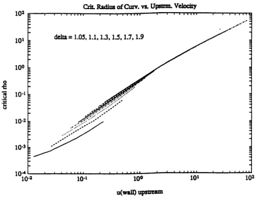
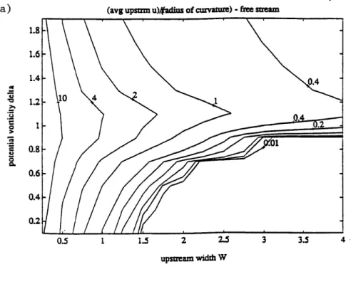
In Chapter 2, the hydraulic model of Roed (1980) and Ou and de Ruijter (1986), and a similar model for barotropic currents, are solved for a range of points in the parameter space controlling the flow. The purpose of obtaining the quantitative relationship between the upstream parameters of the flow and the predicted minimum radius of curvature needed for separation is to allow us to compare the predicted radius of curvature with the actual radius of curvature needed for separation in the experiments of Bormans and Garrett (1989).

Chapter 3 describes results from baroclinic experiments that are similar to those of Miller and Whitehead (1979), Kawasaki and Sugimoto (1984, 1988), and Bormans and Garrett (1989). Whereas those experiments involved density currents flowing around corners at the mouth of a channel, in my experiments the left wall of the channel is removed so that the flow is a coastal current upstream of the corner as well as downstream. While earlier experiments found a critical radius of curvature of the corner for which a gyre was produced, these experiments find a critical corner angle for gyre creation. The experiments also explore how different lower layer depths and different initial conditions affect eddy generation. These experiments obtain quantitative data about the current upstream and downstream of corner.

In the barotropic experiments described in Chapter 4, flows of various strengths are pumped over a sloping bottom and around a corner to see if the separation im-plied by Hughes (1989) actually occurs. In fact eddies are produced by some of these flows for a variety of related topographies, and their characteristics are studied.

Chapter 2.

Hydraulic Models of Separation From

Curved Coastlines

2.1.

Introduction

The separation of a coastal current from a curved boundary in a rotating system has been studied but the dynamics has not been explained. Whitehead and Miller (1979) and Bormans and Garrett (1989) performed laboratory experiments in which a current was created by a dam-break and flowed through a channel into a wider basin, where it either stayed attached to the wall outside the mouth of the channel or separated from the wall to form a growing anticyclonic eddy just outside the channel. The corner was rounded, with a radius of curvature which could be varied relative to both the width and the Rossby radius of the current. Bormans and Garrett's experiments suggest that separation occurs when the radius of curvature is less than the inertial radius of the current, u/f for current speed u and Coriolis parameter

f.

The dependence on the rotation parameter raises the possibility that dynamics unique to a rotating system are involved in the separation of the current.

Roed (1980) and Ou and de Ruijter (1986) gave one possible mechanism for this gyre formation. They studied inviscid, steady state, uniform potential vorticity two-layer flows in which the bottom layer was infinitely deep and hence motionless. Assuming that alongstream variations had a length scale that was long compared to the width of the current allowed them to neglect derivatives with respect to the alongstream coordinate in the equations of motion, so that the partial differential equations became ordinary differential equations with respect to the cross stream coordinate. The only ways in which the curvature of the boundary entered into the equations of motion in this approximation were in a centrifugal term in the force

balance and a curvature term in the potential vorticity equation.

Roed examined a density front (Figure 2.1.1a) along which the current flowed with the wall to its right looking downstream (his and our discussion are confined to systems with counterclockwise rotation), while Ou and de Ruijter studied a current bounded by a wall on its left and a free streamline on its right (Figure 2.1.1c). In both cases, increasing the curvature of the wall, as one traveled downstream from a region of zero curvature, decreased the layer thickness at the wall. At some critical radius of curvature, the thickness became zero. This implies that if a rounded corner has a greater curvature than the critical one, the solution has the physically meaningless property of negative layer thickness at the wall, and it is impossible to have a steady state flow with the current attached to the wall at the bend.

Though these two papers demonstrated that such a behavior exists, they did not show how great a curvature a given upstream flow needs in order to actually separate. In this chapter, I non-dimensionlize the equations somewhat differently than Rsed did, and solve for the critical radius of curvature as a function of the two non-dimensional upstream parameters which control the form of the boundary current. This allows us to compare the different flow cases (front and free stream-line) illustrated in Figure 2.1.1. A thorough examination of parameter space will investigate the possibility that the current may separate due to a flow reversal rather than a surfacing of the interface. Finally the separation criteria derived here can be compared with the experimental results mentioned above. Ultimately, we would like to see if inviscid, centrifugal upwelling can account for flow separation from a wall in

real laboratory and natural systems.

In order to gain a more complete understanding of the influence of cur-vature in the simplified equations of motion, the long wave approximation is also applied to barotropic flows, both with a flat bottom and a sloping bottom. In such systems the momentum equation becomes unnecessary, and the dynamics is governed

density front quiescent layer (a) (b) (c) ' f -I -quiescent layer

AWL

_x wall-on -left quiescent layer

Figure 2.1.1: Upstream current structure for reduced gravity models. (a) Density front case as in Roed (1980). (b) Free streamline case (potential vorticity front only) with wall on the right. (c) Free streamline case with wall on left, as in Ou and de Ruijter (1986).

wall-on-right

z

'Or

9

by the potential vorticity equation alone. For this reason rotation vanishes from the formulation for the flat bottom case, which should display the same dynamics as a two-dimensional, inviscid, non-rotating flow, though rotation reappears in the sloping bottom case through the influence of bottom topography on potential vorticity. In these systems, centrifugal upwelling cannot occur because there is no density interface to upwell. However, it is possible that the current speed at the coast will reverse for a great enough curvature. As in the reduced gravity case (flow above an infinite lower layer), this flow reversal implies that separation of the current from the coast must occur for sufficiently great curvature.

Hughes (1989) showed that a flow reversal does occur for a system with to-pography that deepens exponentially with distance from a coast and with a potential vorticity distribution profile that is an exponential function of the streamfunction. In this chapter, we look at linear topographic slopes and flow profiles that consist of one or two regions of uniform potential vorticity. This formulation is mathemat-ically more simple than that of Hughes, and permits analytical solutions for both upstream (straight coastline) and downstream (curved coastline) velocity profiles. Hughes' continuously varying potential vorticity is perhaps more realistic, but the equations must be numerically integrated to find the flow profile both upstream and downstream (Hughes, 1989). The simplicity of flows with piecewise uniform potential vorticity should also make it easier to compare the flat bottom, sloping bottom, and reduced gravity systems with each other.

In this chapter, we will first derive the system of equations to be solved for all of the cases described above, as well as the appropriate form of the equations and boundary conditions for each case. Separate sections will deal first with the barotropic flat bottom case, then barotropic sloping bottom case, and finally reduced

gravity flows. Though the barotropic sections precede the baroclinic section, the main emphasis of the chapter is on the baroclinic work, because it is the most relevent to real

fluid flows. There are several problematical aspects of the barotropic work which will be discussed below. Most importantly, after I performed the barotropic calculations, analysis of my homogeneous-density laboratory data (see Chapter 4) showed that processes involving vertical shear (which are not included in these shallow water models) were important to the flow separation in homogeneous systems. However, the barotropic results are included here because they do display some interesting nuances of hydraulic theory.

2.2.

The System of Equations to be Solved

Following Roed (1980), we start with the cross-shore component of the mo-mentum equation, and the conservation of potential vorticity, both in curvilinear coordinates. + vv - - + fu =-g'hy, (2.2.1a) 1_{+y/p p~y} VW U -U, +-" + f = qh, (2.2.1b)

1+19

~p+y

where (u, v) are the alongshore and cross-shore components of velocity, (x, y) are

coordinates parallel to and perpendicular to the shore, h is the layer thickness, p is the local radius of curvature of the shore (and the coordinate system), f is the Coriolis parameter, g' is the reduced gravitational acceleration, and q is the potential vorticity. The smaller p is, the larger the curvature, so that for a straight wall, p = oo, and for a sharp corner, p = 0. The wall is at y = 0, and for convex curvature p is positive. For the case in which the wall is on the right of the current looking downstream, we have u > 0, and when the wall is on the left, u < 0. Now let us non-dimensionalize the equations with (u, v) scaled by

(U,

V), h scaled by D, and (x, y) scaled by (p, W).

--

)

(hu)x + -- ([1 + (W/p)y] hv), = 0, (2.2.2)

implies that U/p = V/W. Using this fact, the non-dimensional version of the mo-mentum and potential vorticity equations above become

-- 62U + VVoY - 6 U2 + U = - hy (2.2.3a)

(jj f2

___

]

U'

-+ 6f 1+6

+

u, -J ) (1 - gh/f) , (2.2.3b)

1+6y 1+6y U

where 6 = W/p. If we assume that the Rossby number U/fW is 0(1) and we neglect 62 terms but keep 6 terms, then the dimensional equations can be approximated by

fu - -g'h, 1h= (2.2.4a)

pu

P+ y 9V

uY

+

=

f

- h. (2.2.4b)

p

+

y

These equations are essentially the equations of motion for axisymmetric circular motion. As stated above, these equations, which were also derived by Rsed (1980), are much easier to solve than the full equations of motion because they consist of coupled ordinary differential equations in y rather than partial differential equations in (x, y). Alongshore variations in the flow enter parametrically through p(x). For a barotropic system, h(y) is determined by the topography, which is known, so only the potential vorticity equation is necessary to determine the velocity profile.

The barotropic system is governed by a single first order differential equation, so one boundary condition must be imposed in order to solve for the motion. Since we are only considering coastal currents, we take the fluid to be motionless far away from the wall. Integration of the vorticity equation (2.2.4b) over a vanishingly small interval in y shows that u must be continuous, so that u = 0 on the outer edge of the jet, y = w. The reduced gravity case is equivalent to a second order differential

equation, so two constants of motion are necessary. For the case of a density front, h goes to zero at y = w. In this case the wall must be on the right (u > 0). For the

free streamline case, the assumption of no motion outside the region of anomalous potential vorticity again tells us that u(w) = 0 as in the barotropic case. Now there is an additional constraint that h must also be continuous in order to have finite u, so h(w) = ho, where ho is the thickness of the stagnant water outside the current. For the front case, we fix ho, the layer thickness at the wall, thus supplying a second boundary condition for the equations.

In order to relate the flow structure at various p to the upstream (p = oo) flow we need other properties of the flow that are conserved along streamlines. For a given p, we must find the current width w(p) in order to know the flow field. For the barotropic flow, it is sufficient to use the volume flux within each region of uniform potential vorticity,

b

Q=

u(y)h(y)dy, (2.2.5)

where a(p) and b(p) are the minimum and maximum values of y with the given vorticity. For the reduced gravity case, more information is needed, so we utilize the Bernoulli function, which to the same order of approximation as equations (2.2.4a,b) can be written

1

B = g'h+ -u2 . (2.2.6)

2

At the end of this section we will review the conditions on B necessary to close the problem.

The most convenient scaling for the equations is somewhat different for each of the two barotropic problems and the reduced gravity problem. In the flat bottom barotropic case, velocity can be scaled by some velocity U in the upstream profile, and all lengths can be scaled by the upstream current width W. Therefore u/U is a function of position (y/W, p1W). If the potential vorticity is uniform, there is no

other parameter governing the system. If there are two regions of uniform potential vorticity in the jet, then two parameters are added: the upstream ratio of widths of the two regions, W1

/W

(W1 is width of region closest to the wall), and another parameter which can be expressed in a variety of ways, including the ratio of the two potential vorticities as well as

uo/U,

which is the ratio of the velocity at the wall to velocity at y = W1. With this scaling, the non-dimensional vorticity equation is

U AU

u + - - (2.2.7)

p+y AW' 227

where AU is the non-dimensional change in upstream velocity across a region of uniform vorticity and AW is the non-dimensional width of the region.

When the topography consists of a linear slope with zero fluid depth at the wall, lengths are scaled as before but speed is scaled by Wf. For such a flow with potential vorticity q and bottom slope s, the parameters are a = qWs/f for

each vorticity, and, if there is more than one vorticity region W1

/W.

Thus there is one non-dimensional parameter for uniform q and three parameters if there are two values of q. Specifying the two dimensionless potential vorticities and W1

/W

is equivalent to specifying W1

/W

and the upstream values of u(y = 0) and u(y = W1).

If velocity in the sloping bottom problem is scaled with U = u(Wi) as in the flat

bottom case, rotation still appears in the potential vorticity equation in the form of a Rossby number, U/fW. In contrast, in the flat bottom case

f

only appears inside the expression

f

- qD, so that "planetary" vorticity is merely a part of relative

vorticity in that case. Using different velocity scales as I have done does not affect any quantities besides the magnitude of the velocities. The non-dimensional vorticity equation for this case is

U

UY

+

= 1 - ay. (2.2.8)

In the reduced gravity problem, h is non-dimensionalized by a scale thickness

gravity wave speed VF. For the density front, ho is the upstream layer thickness at the wall, and for the free streamline case, ho is the upstream thickness at the outer edge of the current. The two non-dimensional parameters governing the system are then the upstream non-dimensional width Wf

/v/g1o

and the non-dimensional potential vorticity,

6= q (2.2.9)

f /ho'

Switching to non-dimensional variables, the equations of motion become U 2

u - = -hy (2.2.10a)

U

Uy

+

=- 1 - Sh, (2.2.10b)

p + Y and B is non-dimensionalized by g'ho, so that

12

B2 . _(2.2.11)

At p = oo, the boundary conditions are simply

h(O) = 1, h(W) = 0 (front), (2.2.12a)

h(W) = 1, u(W) = 0 (free streamline), (2.2.12b)

The Bernoulli function B at the streamline adjacent to the coast can be computed upstream, and provides an additional constraint from which to calculate w(p) for finite p. The condition that the front has h(0) = 1 upstream does not hold for finite p, but since the offshore edge of the current is a streamline, the Bernoulli function there can be used instead. To summarize, for flow bounded by a density front we have

12

at y=O0, h

+-gu

= Bo, (2.2.13a)

aty=w, h=0 and -u = B1, (2.2.13b)

and for the free streamline case

12

at y = 0, h+ -u2 = Bo, (2.2.14a) 2

aty=w, h=1 andu=O, (2.2.14b)

where B0 = B(O) and B1 = B(w).

2.3.

Barotropic Flows Over a Flat Bottom

In this section, we will calculate the flow profile for a region of uniform vorticity, and then calculate the flow for a current consisting of two regions of uniform vorticity. All calculations will be performed in the non-dimensional units introduced in the previous section.

Uniform Potential Vorticity

When the coast is straight (p = oo), equation (2.2.7), the condition that

u(W) = 0 and the use of the velocity at the coast as the velocity scale constrain the upstream velocity profile to be simply

u(y) = 1 -y. (2.3.1)

Then the volume flux

Q

(see equation (2.2.5)) is equal to 1/2, and AU/AW = 1 (see equation (2.2.7)).

We can solve (2.2.7) by solving the homogeneous version, which is separable, and then using the method of variation of parameters to solve the inhomogeneous problem. Invoking the outer boundary condition, we find that

U

= .1 '(W2_ 2)+ p( - y)l .(2.3.2)

Since we always have y < w, the current never reverses, so there is never any separation. For completeness, let us find w, which we do by integrating the volume flux (equation (2.2.5)) from y = 0 to y = w and setting the quantity equal to its upstream value:

12 1 plo4 W 1 1

-p2 + -(p + )2 _ln _ (2.3.3)

4 2 p 2 2

which can be rewritten using w' = w/p:

1 + (1 + w'2_{) [21n(1}

₊

_{w') - 1]}

= 2/p 2

. (2.3.4)

The variation of w with p can be displayed by calculating p as a function of w' in equation (2.3.4) and plotting w = w'p against p. The current width decreases monotonically as p decreases from oo. Changes in w are small unless the radius of curvature becomes small compared to the upstream current width, in which case the long wave approximation has already broken down. For all p, u(y) is a monotonic function with a maximum at y = 0, where u = w(1 +

}w/p),

and u(y = 0) increases as the radius of curvature decreases.

The qualitative features of these results can be explained by examining equa-tion (2.2.7). As the boundary curvature increases, the centrifugal term u/(p + y) increases from zero, forcing the shear term Ou/y to decrease. Since for this flow,

Ou/Oy < 0, uly | must increase. Meanwhile the volume flux must remain

con-stant. If the shear is approximated with u(0)/w, and the flux by

Q

= u(0)w, then u(0)/w = u(0)2/Q = Q/W2_{, so that as curvature increases the shear, the current}

be-comes faster and narrower. This analysis has an implicit assumption that the shear is about the same for all y, which happens to be true for all p for which w was calculated.

Two Regions of Uniform Potential Vorticity

The constraint of uniform potential vorticity limits the range of currents which can be modelled. More important, it is conceivable that it limits the range of