HAL Id: halshs-00543971
https://halshs.archives-ouvertes.fr/halshs-00543971
Preprint submitted on 7 Dec 2010HAL is a multi-disciplinary open access archive for the deposit and dissemination of sci-entific research documents, whether they are pub-lished or not. The documents may come from teaching and research institutions in France or abroad, or from public or private research centers.
L’archive ouverte pluridisciplinaire HAL, est destinée au dépôt et à la diffusion de documents scientifiques de niveau recherche, publiés ou non, émanant des établissements d’enseignement et de recherche français ou étrangers, des laboratoires publics ou privés.
Get paid more, work more? Lessons from French
physicians’ labour supply responses to hypothetic fee
increases
Olivier Chanel, Alain Paraponaris, Christel Protière, Bruno Ventelou
To cite this version:
Olivier Chanel, Alain Paraponaris, Christel Protière, Bruno Ventelou. Get paid more, work more? Lessons from French physicians’ labour supply responses to hypothetic fee increases. 2010. �halshs-00543971�
1
GREQAM
Groupement de Recherche en Economie Quantitative d'Aix-Marseille - UMR-CNRS 6579 Ecole des Hautes études en Sciences SocialesUniversités d'Aix-Marseille II et III
Document de Travail
n°2010-52
Get paid more, work more?
Lessons from French physicians’
labour supply responses to
hypothetic fee increases
Olivier CHANEL
Alain PARAPONARIS
Christel PROTIERE
Bruno VENTELOU
December 2010
Get paid more, work more? Lessons from French physicians’
labour supply responses to hypothetic fee increases
Chanel O
(1), Paraponaris A
(2,3,4), Protière C
(2,3,4), Ventelou B
(1,3,4)(1) CNRS, GREQAM UMR 6579, Marseille, F‐13002, France (2) INSERM, UMR 912 (SE4S), Marseille, F‐13006, France (3) Université Aix‐Marseille, IRD, UMR 912, Marseille, F‐13006, France (4) ORS PACA, Observatoire Régional de la Santé, Provence Alpes Côte d’Azur, Marseille, F‐13006, France Abstract
This paper is devoted to the analysis of the General Practitioners’ (GPs) labour supply, specifically focusing on the physicians’ labour supply responses to higher compensations. This analysis is mainly aimed at challenging the reality of a ‘backward bending’ form for the labour supply of GPs. Because GPs’ fees only evolve very slowly and are mainly fixed by the National Health Insurance Fund, we designed a contingent valuation survey in which hypothetical fee increases are randomly submitted to GPs. Empirical evidence from 1,400 French GPs supports the hypothesis of a negative slope for the GPs’ labour supply curve. Therefore, increasing the supply of physicians’ services through an increase in fees is not a feasible policy. Keywords: General practitioners, contingent valuation, price of leisure, labour supply, backward bending curve Financial support was provided by the French Research Institute on Public Health (IReSP), through the Health Services Research Program 2008 There is no conflict of interest. Corresponding author: Christel Protière : ORS PACA / 23 rue Stanislas Torrents / 13006 Marseille / France / christel.protiere@inserm.fr
1. Introduction
In the literature devoted to the valuation of the time spent in leisure and to the consumption-leisure trade-off, the time value is usually considered as a percentage of the wage rate. Indeed, the neoclassical model of the labour-leisure choice assumes that individuals, when choosing the quantities of work and leisure, select the combination that maximises their utility, so that the marginal rate of substitution between labour and leisure equals the hourly wage rate plus the value of an additional hour of leisure. This model is weakened by at least two flaws. First, it requires the following set of necessary assumptions for the labour market: it must be in “pure and perfect competition”, and it must accurately reflect actual individual trade-offs between work and leisure. Second, it implies that there is a sufficient heterogeneity in the data to estimate real changes in behaviour due to price heterogeneity, which is generally collected from regional variations in market prices; but that is obviously not the case in systems where the fee is mainly and uniformly fixed by the national public authorities, i.e., the government or Health Insurance. In France, general practitioners’ (GPs) fees are fixed and capped by the public authority for the numerous physicians who belong to the first of the two payment schedules (sector 1).
When facing a lack of data about market responses to price variations, the economic value of non-market goods can be assessed using two alternative methods. The first one uses behaviour observed on markets related to some characteristics of the good (where preferences are “revealed” through hedonic or travel cost methods), and the second elicits declared preferences concerning the good (“stated” preferences). The most well-known and widely used approach for measuring stated preferences is the contingent valuation (CV), in which respondents are presented with a “constructed market” for the good at stake and they reveal their (hypothetical) behaviour regarding whether or not they would be willing to buy this good and, if so, at what price.
This paper is based on the second approach. It aims to provide results in two connected directions: to explore how a change in fees would affect the supply of medical consultations, and to discover the value of marginal units of leisure (i.e., non professional) activities for GPs. The paper is organised as follows: in section 2, we sketch a theoretical microeconomic model of the medical labour supply, which shows the possibility of a “backward bending” curve for at least some values of the exogenous parameters. In section 3, we discuss empirical issues regarding how to overcome the lack of variations in prices and present the data that was considered in the empirical part of the paper. The results are given in section 4 and section 5 concludes.
2. The theoretical framework: ‘The backward bending curve’ for self
employed GPs
Most often, the lack of time is given by GPs as the main reason for not being able to pay sufficient attention to a set of activities such as counselling, health education, prevention or the consideration of guidelines. In doing so, GPs implicitly make a trade-off between consultation length and consultation fee, suggesting that they use consumption-leisure deliberations. In the standard model, an individual derives utility from the consumption of both leisure and a bundle of goods, as measured through income. The model for independent practices contrasts with the standard model of labour supply in the following characteristics: a
“fee” is paid per consultation, and there is a simultaneous decision regarding the number and the length of consultations. The physician’s choice can be expressed as follows:
MaxU(C,Z) st.C= w.N.x − T Z= Z0− b.N.x ≡ Z0− L N= N(x,b) (1)
where the physician faces:
- a budgetary constraint (for the purchase of goods): C=w.N.x –T; where C represents the
level of consumption, w represents the fee, x represents the number of consultations per patient, N represents the list size and T represents the overall cost of the medical activity;
- a time constraint Z, where Z0 is a fixed time endowment, Z is the amount of time devoted
to leisure and b is the average length of each consultation. Here, the opportunity cost of the supply of health services is the loss of leisure. After denoting the duration devoted to labour by L=b.N.x, we assumed U’L<0.
- a market constraint N (the number of patients): N = N(x, b);
In this model, each physician is considered as a local monopoly. The level of demand addressed to her (the list size) is a function N(x, b) that depends on the amount of services offered (the number of consultations) and the quality of the consultation (b). McGuire (2000) suggested a “net benefit function” for the patient that depends on the medical workload, the level of quality provided by the physician and the competition intensity among suppliers. This net benefit function plays a role similar to our demand function. We considered “quality” and “length of consultation” as equivalent, an assumption already suggested by McGuire (2000) (some quality indexes for GPs’ consultation, for instance, the Consultation Quality Index (CQI), are explicitly based on the consultation length (Howie et al., 2000)). In our labour supply framework, the cost of quality is endogenous: it is defined as the value of the loss in leisure due to the time spent in each consultation (see also Fortin et al., 2010). Formally, the physician’s choice can be expressed as follows:
assuming an optimisation in b and x by the physician, the first order conditions (FOC) are:
⎪
⎩
⎪
⎨
⎧
+
=
−
=
b
w
e
e
U
U
e
b N b N C Z x N / / /1
'
'
1
(2) where eN/b = b b N N / / ∂∂ is the elasticity of N to b and e
N/x is the elasticity of N to x.
The first equation is a key feature of the fee-for-service system: the number of consultations and the number of patients are perfect substitutes. The second equation gives a modified leisure-consumption principle in which the elasticity of the list size to b appears as a parameter. By choosing the total working time and the consultation duration, the physician must internalise the effects of her allocation on the patient’s benefit (the patient’s willingness to remain in her list).1
1 There are similarities with the framework presented in Rochaix (1993), where physicians are assumed to realise
These two equations help compute the equilibrium values of the two interest variables of the program x* and b*, and, consequently, L*= b*x*N(x*,b*) is the physician’s labour supply at equilibrium. As was shown in the first order conditions in (2), the ratio U’Z/U’C, i.e., the
marginal rate of substitution between leisure and consumption, plays a decisive role. It can be illustrated with the help of some specific functions for U and N. If we consider a utility function:
- U(C,L)=(Cφ−1/φ −δ.Lφ−1/φ)φ/φ−1, where δ represents the opportunity cost of time at the
physician level and φ is the usual constant elasticity of substitution (CES) parameter, and if N(x, b)=
b
β(g(x))
α, then the overall cost of activity T can be written as a cost per unit of consultation τ: T=τ.w.x.N. Then, equation (2) becomes:eg / x = −1/
α
b= (1δ
β
1+β
w (w−τ
)1/φ) φ 1−φ ⎧ ⎨ ⎪ ⎩ ⎪At the equilibrium, the GP’s labour supply L*= b*x*N(x*, b*) is then equal to:
) 1 ( 1 / 1 1 1 1 ) ) ( 1 1 ( *) ( *) ( * + + + − + − + = = φ β φ φ α α β τ β β δ w w x g x g b L
A derivative of L* in w reveals that the sign of the relationship between L and w depends on the sign of a term that can be easily discussed: sign * sign
1 L w w
φτ
φ
⎛ ⎞ ∂ ⎛ ⎞ = − − ⎜ ∂ ⎟ ⎜ − ⎟ ⎝ ⎠ ⎝ ⎠.For
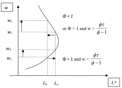
φ
<1 (where leisure and consumption are hardly substitutable), the expression is always negative. Referring to Figure 1, if real wages increase from w1 to w2, then the GP is willing todecrease the hours worked (expressed per day, month, year or even per lifetime) from La to
Lb.
However, if
φ
>1 (the substitution effect is a priori greater than the income effect), the expression becomes positive for a low wage level (an increase of real wages from w3 to w4 inFigure 1 corresponds to an increase in the hours worked from Lb to La) but remains negative
for a high wage level (an increase from w1 to w2).
Then, we get the standard “backward bending curve” for a self-employed physician (Figure 1). The model gives the following insights:
-when the substitution between time and money is low, the GP’s labour supply-payment elasticity can be negative: the greater the fee for the GP’s service, the less the GP works. Intuitively, when money and leisure time are highly complementary, the income effect - due to higher fees - pushes physicians to allocate earnings into more leisure time, thus reducing the labour supply;
they allocate their effort between different procedures/activities on the basis of their relative prices. The main difference consists in assuming that, in the second stage, physicians allocate their effort between the “duration” and the “quantity” of each consultation on the basis of the relative demand elasticity of both terms.
-for high incomes, w > Ω and a negative slope is also likely (for a higher substitutability level between time and money in the utility function).
These results are already well documented in the case of salaried workers (when w is a wage, see for example, Brown and Lapan, 1979), and the present model re-states them in the case of fee-for-service payments.
3 Data
3.1 Empirical issues
Labour economists have paid little attention to the overall labour supply of physicians. The relevant references in the field are: Sloan (1975), Noether (1986), Rizzo and Blumenthal (1994). The last one provides an estimation of the labour supply-earnings elasticity equal to .23, with an adjusted price-elasticity equal to .44. In a study of the response of the physicians’ labour supply to the tax system, Showalter and Thurston (1997) found that self-employed doctors are more sensitive than their salaried counterparts to the marginal rates of taxation, with elasticity equal to .33. A study of Norwegian micro-data by Sæther (2006) confirms that the response of wage-earning hospital doctors is low. The most recent studies used panel data from Norway and found a long-run wage elasticity equal to .3, a figure which could be viewed as higher than the ones provided by studies conducted in the US, given that doctors in Norway are salaried (Baltagi et al., 2005). Ikenwilo and Scott (2008) offer a renewed approach through integrating degrees in job quality as an alternative explanation for wage differences.2 The results are sensitive to the exclusion of the quality of medical services. They slightly underestimate the uncompensated earnings elasticity as being equal to .09 when the quality of physicians’ services is controlled for and as being equal to .12 when it is not. Replicating these empirical results in France is problematic, as there is no real variability in the fees paid to the population of self-employed GPs. The French health system is regulated by the public authority, which set up fees paid per consultation (22€ in October 2010) for 93% of the GPs (Secteur I)3. Therefore, in order to explore how GPs’labour supply may respond to higher fees, we implemented a contingent valuation (CV) survey in which hypothetic offers (variations in fees) are submitted to a representative sample of French GPs. If properly implemented, it has been proven that CV surveys provide reasonable values for non-market goods and non-use values in the environmental and health fields.
3.2 Data collection
The GPs’ sample is made up of a panel survey undertaken in March 2007, which examines the professional environments and practices of 1,901 GPs in five French regions: Basse– Normandie, Bourgogne, Bretagne, Pays de Loire and Provence-Alpes-Côte d'Azur. The panel was compiled from a joint initiative of the Ministry of Health, the National Federation of the Regional Health Observatories (FNORS) and the Regional Unions of Self-employed Doctors (URML) in the regions considered. In each region, the respondent GPs are representative of
2 A key issue is the lack of attention paid to the role of non-pecuniary factors in influencing labour supply. This
stems from a concern about unobserved heterogeneity in models where hourly wages have been shown to have a negligible impact on the labour supply, and where workers may choose to increase or reduce their working times in response to changes in non-pecuniary factors. These factors are usually unobserved by researchers, and they may be correlated with the included independent variables, leading to a bias due to omitted variables.
3 The remaining 7% can set their fees freely (Secteur II). In compensation, social taxes on physicians’ earnings
the overall GPs’ population (see Aulagnier et al., 2007). The sample was obtained by a random stratified sampling with the strata defined by gender, age (the categories in 2006 having been under 45, 45-54 and 54 and older) and location (urban, suburban, rural). Doctors planning to either stop practising or to move out of the region were excluded, as were those who practised exclusively alternative medicines such as homeopathy and acupuncture. The first survey wave took place in March and April 2007, and the data collected from GPs concerned their levels of activity, such as the workload, list size and the number and type of consultations. This wave also includes data from the Individual Receipt for Activity and Prescribing (RIAP), an administrative document given to GPs by the Health Insurance, which records all reimbursed spending of patients and gives the precise computations of the activities of each GP.
To explore GPs’ behaviour regarding the trade-off between income and leisure, we asked GPs how they would change their quantity of labour (the number of hours worked and the average duration of a consultation) in reaction to changes in the current fee paid per consultation. One increase among three has been randomly proposed to each GP: 5%, 10% or 20%. Note that letting the quantity of labour and the average duration of each consultation remain unchanged automatically results in a similar increase (of 5%, 10% or 20%) of their earnings.
This approach differs from the standard way non-market goods are elicited in CV. Indeed, the usual wording is typically about how much people are willing to pay for a change in the quantity or the quality of a good at stake (see, for instance, Dalenberg et al., 2004 for a direct measurement of the values of different leisure activities). By proposing a price (the fee increases), the wording used in our survey purposely imposes no a priori regarding the direction of the changes, which can differ for individuals due to their distinct motivations and tastes, as seen in section 2 (and the direction of change could be either positive or negative, depending on the value of the slope dL/dw). Indeed, by assuming that the level of utility before the change in fees reflects the optimum level of each GP, we were able to determine the trade-off between a change in income and a change in the quantity of leisure consumed, i.e., we were able to estimate the marginal “shadow” or “implicit” price of leisure.
4 Results
4.1 Sample
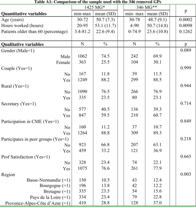
Of the initial sample of 1,901 GPs, 130 GPs (6.9%) who do not belong to Secteur I (GPs who apply the regulated fees) were removed, as were 346 respondents who either did not answer key questions (regarding the number of hours worked and the number of consultations) or whose answers were surprisingly high or low for the variables relevant in the analysis (a change of more than 50% in the number of hours worked, the average duration of the consultation being shorter than five minutes, weak activity, etc.). The remainder of the sample then consisted of 1,425 out of 1,771 GPs belonging to Secteur 1 (or 80.46% of this initial sample). The descriptive statistics related to the sample considered in this paper, as well as tests for equality with regard to the removed GPs, are provided in Appendix 1 (the noticeable difference between the samples is a lesser length of activity for the 346 removed GPs, and can be explained by the fact that weak activity, less than 20 hours per week in practice, was a criterion to exclude GPs from the sample).
Two variables are interesting for the public decision–maker in a centralised health system (like France) or for private decision-makers in a large health insurance coverage system (the US health system, for instance) looking for an increase in the supply of medical services: the
elasticity of the number of hours worked to the level of the fee ELT and the elasticity of the
medical supply (number of procedures) to the level of the fee EN*T.
The former is computed as ELT=(ΔL/L)/( Δw/w), where L is the number of hours worked, ΔL
the change in the number of hours worked, w is the level of fee having been reimbursed at the time of the survey and Δw is the increase in level of fee proposed in the scenario (5% ,10% or 20%). The details of the computations that lead to the latter are provided in Appendix 2. ELT gives the positions of GPs on the backward bending curve and EN*T indicates whether or
not an increase in fees is going to increase the supply, in other words, whether or not fees are a useful instrument to induce a higher medical supply.
4.2 Descriptive statistics pertaining to elasticity
Let us first consider ELT the elasticity of the number of hours worked to the level of the fee. GPs expressed a change in the number of hours worked in 441 out of 1,425 cases (30.95%), and there were no changes in the remaining 984 cases (69.05%). Among those who would change their hours, 422 GPs expressed a hypothetical decrease and 19 GPs expressed a hypothetical increase in their working time. Hence, most of the GPs are either in the vertical part (null elasticity) or in the backward part (negative elasticity) of the labour supply curve. That is not surprising, as it is known that leisure is not an “inferior good” and that GPs have, on average, a higher income than other workers. Figure 2 outlines the distribution.
When we computed the elasticity of the number of hours that GPs would work relative to the fee level ELT, we obtained an average of -.397. After computing the elasticities by scenario,
we found elasticities of -.504, -.394 and -.288 for corresponding changes of 5%, 10% and 20% in the fee level, respectively. The mean elasticity obtained in the 20% change scenario is significantly and substantially higher than in the 5% change scenario (two sample two-tailed comparison mean, with a p=.001) and in the 10% change scenario (with p=.017). Moreover, there is no statistically significant difference in WTP elasticities for the 5% change and 10% change scenarios (p=.126).
This result indicates that the average change in the number of hours worked decreases with the magnitude of the change in the fees, in other words, that there is a marginal decrease in elasticity.
Let us now consider the elasticity of the number of acts offered to the level of fee EN*T. Note
that because the data do not enable one to distinguish the number of consultations per patient (x) and the number of patients (N), we are only interested in the number of acts N*=L/b (N*=x.N in the theoretical model).
In addition to a change in the duration of their labour, GPs were also allowed to state changes in b, the duration of consultations. Whereas 1,237 out of 1,425 GPs (86.81%) declared no change in the duration, 179 out of 1,425 (12.56 %) GPs declared an increase in the duration, and 9 GPs (0.63%) declared a decrease in the duration. Hence, the declared number of acts N*=x.N resulted both from changes in the number of hours worked and changes in the consultations’ durations. In 514 out of 1,425 cases (36.07%), fee increases resulted in a change in the number of acts, and there were no changes in the remaining 911 cases (63.93%). Among the non-null changes, 491 GPs expressed a decrease and 23 GPs expressed an increase in the number of acts. It then appears that most of the GPs declared themselves willing to provide fewer acts than they currently do when proposed with an increase in the level of their fees.
When we computed the elasticity of the number of acts to the level of fee EN*T, we obtained
an average of -.589 (Figure 3). After computing the elasticities by scenario, we found elasticities of -.696, -.605 and -.461 for changes of 5%, 10% and 20% in the fee level, respectively. The mean elasticity obtained in the 20% change scenario is significantly and substantially higher than in the 5% change scenario (p=.0074) and the 10% change scenario (with p=.024). There are no significant differences between the elasticity WTP for the 5% change and 10% change scenarios (p=0.339). Here again, these results indicate that the change in the number of consultations is marginally decreasing with the change in the fee level.
4.3 Estimation results
So far, we have only considered changes in the mean elasticities or only taken into account differences due to the different scenarios proposed to GPs. In order to take into account GPs' heterogeneity and to find out whether some GPs’ characteristics may explain their choices for the duration of their work or their workload, we now turn to regressions analyses.
Much microeconomic data collecting behavioural changes, including our dataset, are characterised by a large amount of null data, and we face the issue of correctly accounting for this specific shape of the distribution. Madden (2008) considers two options: sample selection and two-part models. In the domain of health behaviour, he notes that the observation of consumption can be caused by two different decisions: a participation decision and a consumption decision.4
Depending on whether independence between the error terms of the participation decision and the consumption decision is assumed, the Heckman Selection model (correlation) or the Two-part Model (no correlation) is relevant. The former requires a two-step (or a maximum likelihood) estimation of the correlation, whereas the latter can be estimated with a Probit for participation and an OLS for consumption.
As we could not reject the null assumption of nullity of the correlation coefficient in the Heckman model (the Wald test for a null correlation leads to a p-value of 0.596), we chose to estimate a two part model. The first equation is a Probit, which reflects the decision to change the number of hours worked, and the second equation is an OLS equation explaining the values taken by the elasticities for non-null answers.
The set of explanatory variables contains the following variables:
- socio-economic variables exogenous to the GPs’ decisions: age, gender, the scenario proposed (5%; 10%; 20%), living as a couple, the proportion of patients aged 60 and older and the proportion of patients with special health insurance (free healthcare because of low income);
- variables related to professional long-term decisions: having a medical secretary, having a group practice, location (rural, urban, suburban), region or practice (among five French regions) and the declared reasons for choosing the place of practice (lack of GPs’ services supply in the practice area or monetary incentives);
4 His paper considers the cases of smoking and drinking, in which individuals may decide not to smoke (drink)
no matter how cheap cigarettes (alcohol) are (this is the participation decision). On the other hand, some smokers (drinkers) may decide not to smoke because each cigarette (alcohol) is too expensive, or due to low income (this is the consumption decision).
- variables related to professional short-term decisions: having obtained another medical diploma, participation in continuous medical education (CME), the supply of free consultations, participation in peer groups for quality benchmarks and the number of hours GPs are used to working in a week;
- self-assessed criteria that may affect professional short-term decisions: the self-assessed level of wealth and the self-assessed level of satisfaction regarding the GPs’ own professional activity.
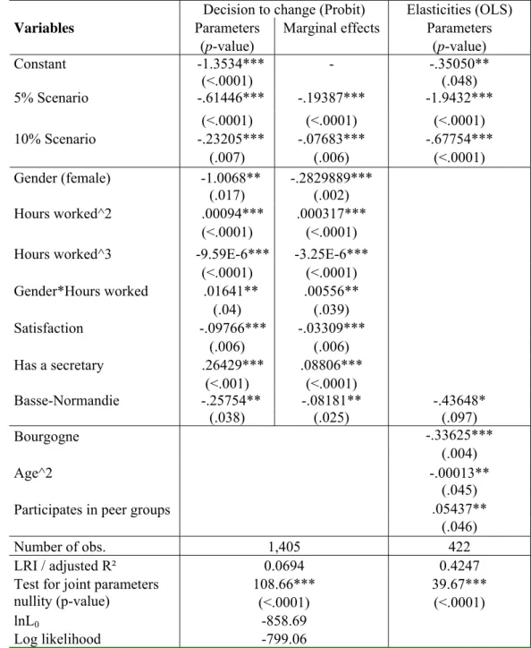
The econometric estimates for the elasticity of the number of hours worked to the fee levels are given in Table 1. Huber-White standard errors were computed to account for possible heteroscedasticity. Because the number of positive values (the increase of hours worked) is very low in the sample (1.33%), we decided to discard the corresponding observations in the following.5 We present the most parsimonious model with variables whose estimated parameter p-values are lower than .1. Note that because the equation modelling the decision to change is a Probit, i.e., a nonlinear model, the marginal effects differ with GPs’ characteristics. We computed them, and they can be found in the third column at the mean values of the explanatory variables. They account for the continuous or discrete nature of the explanatory variables at stake. For the equation explaining the elasticity, Ordinary Least Squares are used and the marginal effects are obviously equal to the estimated parameters. The first column in Table 1 presents the results of the decision to change the number of hours worked. It could be connected to a study of the location of GPs within Figure 1 showing the ‘backward bending curve’. Roughly speaking, GPs can be at the middle of the curve (showing no reaction in L) or above this intermediate area (a negative reaction in L).
First, it is worth noting that the type of scenario proposed is highly significant and negatively related to a change in the worked hours: the marginal probability of a change is almost 20% (resp., 7.7%) lower for a 5% (resp., 10%) increase in the level of fees than for a 20% increase. Thus, the fact that the willingness to change increases with the change proposed in the fee can be considered as a reassuring result, for it provides evidence of the internal validity of the method (in line with the results generally found with respect to income in CV surveys, for instance, see Bishop and Woodward, 1995).
Turning to the effects of the other significant variables, we observe the following coherent results: the coefficient associated with Gender is significant and negative, meaning that women are less likely to decide to change the number of hours worked. Indeed, being female decreases the probability to change by 28%. This result is in line with what we know regarding French female GPs: there is a 5 to 10 hour gap between female GPs and their male counterparts in the French regions (Aulagnier et al., 2007), which reflects the fact that their working time is the product of collective decisions at the household level (Bourguignon et Chiappori, 1992). Neither slight nor substantial changes in fees make them reconsider their original choice. This interpretation is supported by the results of the estimation of the same model where two alternative interaction variables are introduced: women living in couples on the one hand, and women living in a couple with a sizeable working time on the other. In that model, the marginal effect associated with women living in couples is negative (it reduces the
5 Note that we have also estimated an ordered Probit model to account for the GPs that declare an increase in the
number of the hours they worked, but the results were very sensitive to the model specification, and did not lead to very different results anyway.
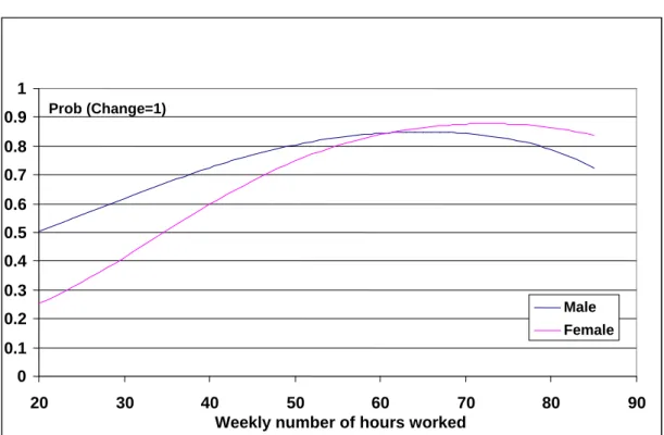
likelihood of a change in the working time) and the one associated with women with high working times is positive (improves willingness to change the number of hours worked).6 Regarding the variables specific to the professional activity, only the number of hours worked in a week has a significant influence on the probability to change. However, its effect is not easy to interpret, due to nonlinearity and the fact that it is gender-dependent (being as it is stronger for female). We therefore represented its effect in Figure 4 by gender, where the probability of changing is computed over the entire range of the number of hours weekly worked (i.e., from 20 to 85), and at the mean values for all the other explanatory variables. We observed that the marginal effect of the number of hours worked follows an inverted-U relationship for both genders (an increase in the number of hours worked increases the probability of changing up to 60 hours for males and 70 hours for females, and further increases in hours decreases the probability). Finally, having a medical secretary significantly increases the likelihood of a change by 8.8% whereas self-assessed level of satisfaction
regarding the GPs’ own professional activity (resp., living in Basse-Normandie) significantly
decreases the likelihood of a change by 3.3% (resp., 8.2%).
Turning now to the determinants of the elasticity in the fourth column of Table 1, we also found that the type of scenario proposed is highly significant and negatively related to the level of elasticity. This confirms that the elasticity is negative with a marginal decreasing pattern: a change of 1€ in the fee level proposed in the 5% Scenario implies a higher negative effect on the number of hours worked than the same change in the 10% Scenario. The effect of the variable Age is decreasing in a quadratic pattern: the older the respondent is, the lower the negative elasticity is. An increase of one unit in the participation in peer groups induces a significant increase of elasticity. Finally, when compared to their counterparts living in the other regions, GPs living in Basse-Normandie and Bourgogne exhibited a decrease in elasticity.
The results of the decision to change the number of acts as well as the elasticity of the medical supply (the number of procedures) to the level of the fee, referred to as EN*T, are provided in
Appendix 2. They are, to a large extent, comparable to the results discussed in that section.
5.4 To a monetary assessment of leisure
If we assume that GPs freely choose the quantities of work and leisure that maximise their utility, the marginal rate of substitution between labour and leisure indicates the value of an additional hour of leisure. To that purpose, we need to distinguish GPs who declare themselves willing to change the amount of hours worked from GPs declaring that they are not willing to change.
For the 422 respondents who declared themselves willing to change the amount of hours worked in reaction to a change in the fee Δw, the overall associated change in the weekly income (also accounting for a change in the mean duration of the consultation, if declared by the GP) is:
6 This interpretation is also supported by the results in appendix 2, which deal with the elasticity of the medical
supply to the level of fees. Indeed, ceteris paribus, being a woman in a couple decreases the probability of a change.
ΔC = Δw N* + ΔN* w + Δw ΔN*
= Δw N* + {[(L+ΔL)/(b+Δb)]‐ L/b }(w + Δw)
The value of an hour of leisure is the trade-off the GP makes between a change in income and a change in the worked hours: Vl = ΔC/ ΔL.
The computation of the value of an hour of leisure for the 422 practitioners who declared a non-null ΔL results in an estimation of €49.79 per hour. By scenarios, we found €56.23, €56.12 and €41.39 for changes of 5%, 10% and 20% in the fee level, respectively, with no significant differences in each case. Although these results, on average, lie in a plausible range, a careful analysis of the distribution (Figure 5) indicates that 18.5% of the hourly values of leisure take a negative value, which seems counter-intuitive. Further explorations are then required to determine whether these negative values are due to non-optimal behaviours in reaction to a change in the fee or for other reasons.
For the 984 respondents who declared no change in the amount of hours worked in reaction to a fee change (Δw), the value of an hour of leisure cannot be computed as it was above, as ΔL=0. However, because it is at the equilibrium, it can be estimated as the GPs’ hourly wage. GPs are free to choose between leisure and work, so that their hourly wage and the hourly value of their leisure should be equal. Note that some GPs can consider the number of hours they work to be out of their control and, hence, decide to keep their current number. The distribution is provided in Figure 6, and it does not strongly differ from the previous one. The mean value of an hour of leisure was €56.99 in this case.
6 Conclusion
The public decision-maker should be able to assess and compare several possible public policies before implementing the one that generates the highest expected welfare in the population. This requires the computation of the optimal reaction of agents to alternative decisions, an issue Contingent Valuation methods could help to deal with by better predicting the behaviour of agents facing changes in their economic environments. For instance, a way to increase the supply of medical services could consist of increasing fees. However, this policy could be double-edged if, statistically, GPs prefer to keep their income constant by decreasing the number of hours worked (i.e., if, on average, the value of their marginal earnings was lower than the value of their leisure). Indeed, we have a strong concern about how GPs would react and adjust their supply when facing variations in their fees. From this perspective, the results of this paper are informative. We found that most of the French GPs are in the vertical part (null elasticity) of the labour supply curve, where the income effect clearly dominates the substitution effect. Even more, some of them are in the backward part (negative elasticity), which is not surprising since leisure is not an “inferior good” and GPs have, on average, a high income (66,800€ in the year 2007 for self-employed GPs, see Fréchou and Guillaumat-Tailliet, 2009).
These results might be important for the design of policies that intend to produce an increase in the labour supply of French physicians: the leverage of the consultation-fee does not seem to offer great perspectives in the supply of physicians’ services, both in quantity and in quality (estimated with the help of the consultation length). A possible alternative is to influence T, the fixed-cost for a medical activity, which seems to play a less ambiguous role in the theoretical model than fees do. Note that these results, although obtained for French GPs,
might be generalised to other contexts: public systems of health insurances, of course, but also private systems in which the health insurer intends to manage the medical workforce and tries to determine the incentive contracts with doctors.
In this paper, we used data where a set of already practising physicians was interviewed, implicitly assuming that the number of physicians in each area of practice was given. Of course, it is possible that, in the long run, the level of consultation fees plays a positive role in the number of physicians set up in family practice or in the localisation of physicians in French sub-regions. However, this positive role may be compensated for by the opposite effect of a reduced supply of health services, as shown by our results. Thus, one of the implications of the present study is that the decision-maker should look for a second instrument in order to control the size of the health service supply across the territory, like incentives to some specific location (rural), or tax exemptions for a given duration after installation. The fee levels (paid per consultation), as unique monetary incentives, seem to demonstrate ambiguous effects.
Finally, an interesting area of future research would be to compare the declared behaviours of the practitioners in reaction to a hypothetical change in the fee with their actual behaviours in reaction to a real change.
Acknowledgement
The authors sincerely thank all the GPs who took part in the survey and all the members of the task groups and steering committee: DREES-Ministry of Health, National Federation of Health Regional Observatories (FNORS), Health Regional Observatories and Regional Self-Employed Physicians Unions in Basse-Normandie, Bourgogne, Bretagne, Pays de la Loire and Provence-Alpes-Côte d’Azur. They also thank Sophie Rolland for research assistance.
References
Aulagnier M, Obadia Y, Paraponaris A, Saliba-Serre B, Ventelou B, Verger P and Guillaumat-Tailliet, F (2007). "L’exercice de la médecine générale libérale. Premiers résultats d’un panel dans cinq régions françaises." DREES. Etudes et Résultats 610. Baltagi B.H. & Espen B. & Holmås, T.H. (2005). A panel data study of physicians' labor
supply: the case of Norway. Health Economics 14:10, 1035-1045.
Bishop, R., and Woodward RT (1995). “Valuation of Environmental Amenities under Certainty”. In Bromley DW ed. Handbook of Environmental Economics, 543--67. Oxford: Blackwell Publishers.
Brown D.M., Lapan, H.E., 1979, the supply of physician services, Economic Inquiry, Volume 17, Issue 2, pages 269–279.
Bourguignon, F. and P. A. Chiappori (1992). "Collective Models of Household Behavior: An Introduction", European Economic Review 36: 355-364.
Dalenberg D., Fitzgerald L., Schuck E. and Wicks J. (2004) “How Much Is Leisure Worth? Direct Measurement with Contingent Valuation”, Review of Economics of the
Household 2, 351–365.
Feather P. and D. Shaw (1999) “Estimating the Cost of Leisure Time for Recreation Demand Models”, Journal of Environmental Economics and Management, 38, 49-65.
Fortin, B., Jacquemet, N., and B. Shearer. (2010). Policy Analysis in the health-services market: accounting for quality and quantity, Annales d’Economie et de Statistiques, Forthcoming.
Fréchou, H., and F. Guillaumat-Tailliet. (2009), Les revenus libéraux des médecins en 2006 et 2007, Etudes et Résultats, n°686, DREES, avril.
Howie JGR, Heaney DJ, Maxwell M, Walker JJ, and GK Freemana (2000) Developing a consultation quality index for use in general practice. Family Practice 17(6), 455-461 Ikenwilo, D. and A Scott. (2008) The effects of pay and job satisfaction on the labour supply
of hospital consultants. Health Economics 16:12, 1303-1318.
McGuire, T., (2000) Physician Agency, in Culyer, A., Newhouse J.P., ed., The Handbook of
Health Economics. North-Holland.
Madden, D. (2008) “Sample selection versus two-part models revisited: The case of female smoking and drinking”, Journal of Health Economics, 27(2): 300-307.
Noether, M., (1986) The growing supply of physicians: has the market become more competitive? Journal of Labor Economics, 4: 503-537.
Rizzo, J.A. and Blumenthal D., (1994) Physician labor supply: Do income effects matter?
Journal of Health Economics, 12: 433-53.
Rochaix L. (1993). Financial Incentives for Physicians: The Québec Experience. Health Economics, 2(2): 163-176
Sæther, E.M., (2006) Physicians' Labour Supply: The Wage Impact on Hours and Practice Combinations. Labour 19:4, 673-703.
Scott, A. (2001) Eliciting GPs' preferences for pecuniary and non-pecuniary job characteristics, Journal of Health Economics. 20:329-347.
Showalter, M. H. and Thurston, N. K., (1997) Taxes and labor supply of high-income physicians. Journal of Public Economics, 66: 73-97.
Sloan, F. (1975) Physician supply behavior in the short run. Industrial and Labor Relations
Table 1: Estimation results (E
LT)
Decision to change (Probit) Elasticities (OLS)
Variables Parameters
(p-value)
Marginal effects Parameters (p-value) -1.3534*** - -.35050** Constant (<.0001) (.048) -.61446*** -.19387*** -1.9432*** 5% Scenario (<.0001) (<.0001) (<.0001) -.23205*** -.07683*** -.67754*** 10% Scenario (.007) (.006) (<.0001) -1.0068** -.2829889*** Gender (female) (.017) (.002) .00094*** .000317*** Hours worked^2 (<.0001) (<.0001) -9.59E-6*** -3.25E-6*** Hours worked^3 (<.0001) (<.0001) .01641** .00556** Gender*Hours worked (.04) (.039) Satisfaction -.09766*** -.03309*** (.006) (.006) Has a secretary .26429*** .08806*** (<.001) (<.0001) Basse-Normandie -.25754** -.08181** -.43648* (.038) (.025) (.097) Bourgogne -.33625*** (.004) Age^2 -.00013** (.045) Participates in peer groups .05437**
(.046)
Number of obs. 1,405 422
LRI / adjusted R² 0.0694 0.4247 Test for joint parameters
nullity (p-value) 108.66*** (<.0001) 39.67*** (<.0001) lnL0 -858.69 Log likelihood -799.06
Significance of estimated parameters and marginal effects: *** if p-value <0.01, ** if p-value <0.05, * if p-value <0.1.
The Likelihood Ratio Index is computed as: 1-(logL/logL0), where logL0 is the value of the
log- likelihood in a model with a constant only.
Figure 1: The backward bending curve
Figure 2 Distribution of E
LT 0 20 0 40 0 60 0 80 0 10 00 F req ue nc y -10 -5 0 5Elasticity of the number of hours worked to the tariff
w L* Φ > 1 and w < 1 −
φ
φτ
Φ < 1 or Φ > 1 and w > 1 −φ
φτ
w2 w1 w4 w3 Lb LaFigure 3 Distribution of E
N*T0 20 0 40 0 60 0 80 0 10 00 F req ue nc y -10 -5 0 5
Elasticity of the number of consultations to the tariff
Figure 4: Effect of the number of hours worked on the decision to
change.
0 0.1 0.2 0.3 0.4 0.5 0.6 0.7 0.8 0.9 1 20 30 40 50 60 70 80 90Weekly number of hours worked
Male Female Prob (Change=1)
Figure 5 The hourly values of leisure for GPs changing the amount of
hours worked (n=422)
0 20 40 60 80 10 0 Fr e q u e n c y -200 0 200 400 600Implicit value of an hour of leisure (in euros)
Figure 6 The hourly value of leisure for GPs not changing the amount
of hours worked (n=984)
0 50 10 0 15 0 20 0 F req ue ncy 0 50 100 150 200 250Implicit value of an hour of leisure (in euros)
Appendix 1. Comparison of GPs’ samples
Table A1: Comparison of the sample used with the 346 removed GPs
1425 MG* 346 MG**
Quantitative variables min-max mean (SD) min- max mean (SD) p
Age (years) 30-72 50.7 (7.3) 30-78 48.7 (9.1) 0.0002 Hours worked (hours) 20-95 53.1 (11.7) 4-90 50.7 (14.8) 0.0098 Patients older than 60 (percentage) 3.4-81.2 22.6 (9.4) 0-74.9 23.6 (10.8) 0.1262
Qualitative variables N % N % p Gender (Male=1) 0.089 Male 1062 74.5 242 69.9 Female 363 25.5 104 30.1 Couple (Yes=1) 0.999 No 167 11.8 39 11.5 Yes 1249 88.2 299 88.5 Rural (Yes=1) 0.944 No 1090 76.5 266 76.9 Yes 335 23.5 80 23.1 Secretary (Yes=1) 0.714 No 577 40.5 136 39.3 Yes 847 59.5 210 60.7 Participation in CME (Yes=1) 0.849
No 160 11.2 37 10.7
Yes 1264 88.8 309 89.3 Participates in peer groups (Yes=1) 0.218
No 923 66.8 207 63.1 Yes 459 33.2 121 36.9
Prof Satisfaction (Yes=1) 0.665
No 328 23.4 74 22.1 Yes 1075 76.6 261 77.9 Region 0.003 Basse-Normandie (=1) 150 10.5 43 12.4 Bourgogne (=1) 196 13.8 42 12.2 Bretagne (=1) 335 23.5 54 15.6 Pays de la Loire (=1) 334 23.4 79 22.8 Provence-Alpes-Côte d’Azur (=1) 410 28.8 128 37.0
Removed GPs = 346 respondents who did not answer key questions (regarding the number of hours worked or the number of consultations) or whose answers were surprisingly high or low for the variables relevant in the analysis (a change of more than 50% in the number of hours worked, a duration of the consultation that was shorter than five minutes, etc.). CME= continuous medical education
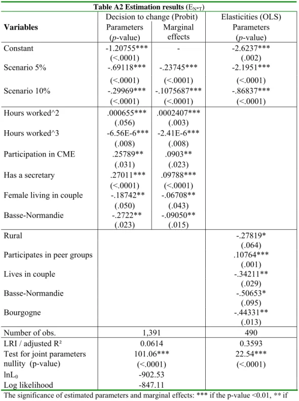
Appendix 2 The elasticity of the medical supply to the level of fees E
N*T
The elasticity of the medical supply (the number of procedures) to the level of fees, referred to as EN*T, is also an interesting variable for a public decision–maker looking for an increase in
the medical supply. The change in the number of acts is the difference between the declared number of acts after the scenario and the actual number of acts:
ΔN*= [(L+ΔL)/(b+Δb)]‐ L/b
with L being the number of hours worked, b being the average declared duration of a consultation, ΔL being the change in the number of hours worked and Δb being the change in the duration of each consultation.
The elasticity of the number of hours worked to the level of fees is then EN*T=(ΔN*/N*)/(Δw/w), where w is the level of fees that was reimbursed at the time of the
survey and Δw is the increase in the level of fees that was proposed in the scenario (i.e., 5% ,10% or 20%). EN indicates whether an increase in fees is going to increase the supply,
i.e., whether fees constitute a relevant instrument to induce a higher medical supply.
As for the elasticity of the number of hours worked to the level of fee ELT, Huber White
standard errors are computed and only the most parsimonious model is presented below. The first column in Table A1 presents the results of the decision to change the number of acts. First, it is worth noting that, as previously found, the type of scenario proposed is highly significant and negatively related to a change: the marginal probability to change is 23.7% (resp. 10.7%) lower for a 5% (resp. 10%) increase in the fee than for a 20% increase. The effect of the weekly number of hours worked has a significant influence on the probability of a change: the marginal effect of the number of hours worked follows an inverted-U relationship with no significant gender differences (an increase in the number of hours worked increases the probability of changing up to 67 hours and then decreases it). Being a female living in a couple decreases the likelihood of a change by 6.7% compared to single females and to all males. Regarding the variables specific to the professional activity, participation to
formation and having a medical secretary increases the probability of a change by 9.03%, and
9.79%, respectively. The geographical phenomenon remains, as GPs living in
Basse-Normandie are less likely to change (9.5%) than their colleagues living in one of the four
other regions.
Finally, as for the determinants of the elasticity in the fourth column of Table A1, we also found that the type of Scenario proposed was highly significant and negatively related to the level of elasticity. The effect of the weekly number of hours worked also has a significant influence on the probability of a change that follows an inverted-U relationship (maximum at 56 hours). Living in a Couple decreases the elasticity (compared to being a single GP) as well as living in Rural areas (compared to urban and suburban areas). Participation in peer groups induces a significant increase in the elasticity of the number of acts to the fee by 10.76%. Finally, when compared to GPs living in other regions, GPs living in Basse Normandie as well as Bourgogne have a significantly (a comparable) lower elasticity.
Table A2 Estimation results (EN*T)
Decision to change (Probit) Elasticities (OLS)
Variables Parameters (p-value) Marginal effects Parameters (p-value) -1.20755*** - -2.6237*** Constant (<.0001) (.002) -.69118*** -.23745*** -2.1951*** Scenario 5% (<.0001) (<.0001) (<.0001) -.29969*** -.1075687*** -.86837*** Scenario 10% (<.0001) (<.0001) (<.0001) .000655*** .0002407*** Hours worked^2 (.056) (.003) -6.56E-6*** -2.41E-6*** Hours worked^3 (.008) (.008) .25789** .0903** Participation in CME (.031) (.023) Has a secretary .27011*** .09788*** (<.0001) (<.0001)
Female living in couple -.18742** -.06708**
(.050) (.043)
Basse-Normandie -.2722** -.09050**
(.023) (.015)
Rural -.27819*
(.064)
Participates in peer groups .10764***
(.001) Lives in couple -.34211** (.029) Basse-Normandie -.50653* (.095) Bourgogne -.44331** (.013) Number of obs. 1,391 490 LRI / adjusted R² 0.0614 0.3593 Test for joint parameters
nullity (p-value) 101.06*** (<.0001) 22.54*** (<.0001) lnL0 -902.53 Log likelihood -847.11
The significance of estimated parameters and marginal effects: *** if the p-value <0.01, ** if the p-value <0.05, * if the p-value <0.1.
The Likelihood Ratio Index is computed as: 1-(logL/logL0), where logL0 is the value of the
log- likelihood in a model with only a constant.