Dielectometry measurements of moisture dynamics in oil-impregnated pressboard

Dielectrometry Measurements of Moisture

Dynamics in Oil-Impregnated Pressboard

by

Yanko Konstantinov Sheiretov

B.S., Massachusetts Institute of Technology (1992)

Submitted to the

Department of Electrical Engineering and Computer Science

in partial fulfillment of the requirements for the degrees of

Master of Science in Electrical Engineering

and

Electrical Engineer

at the

MASSACHUSETTS INSTITUTE OF TECHNOLOGY

May 1994

© Yanko Konstantinov Sheiretov, MCMXCIV. All rights reserved.

The author hereby grants to MIT permission to reproduce and

distribute publicly paper and electronic copies of this thesis

document in whole or in part, and to grant others the right to do so.

Author

...

...

Departme

of Electrical Engineering and Computer Science

May 11, 1994

Certified

by/... ..

a.

.... ...

Markus Zahn

Professor of Electiief Engineering and Computer Science

Thesis Supervisor

M

ASSASC"tI,8

,:

ATIY*-

..

..

T..

Dielectrometry Measurements of Moisture Dynamics in

Oil-Impregnated Pressboard

by

Yanko Konstantinov Sheiretov

Submitted to the Department of Electrical Engineering and Computer Science on May 11, 1994, in partial fulfillment of the

requirements for the degrees of Master of Science in Electrical Engineering

and

Electrical Engineer

Abstract

The dielectric spectrum of pressboard is a function of its moisture content and temper-ature. The real component of the complex permittivity gives the dielectric constant while the imaginary component characterizes the power dissipation in the material. In oil-impregnated pressboard of medium and low humidity the dielectric spectrum's shape and amplitude do not change with variations in temperature and moisture con-tent, but only shift in frequency. Thus it is possible to create a universal curve, with appropriate temperature correction factors, which can be used to extract informa-tion about the moisture dynamics of solid transformer insulainforma-tion from dielectrometry measurements.

Such measurements may be taken with the material placed in a parallel-plate lossy capacitor structure whose complex impedance is measured. In this way one obtains values for the complex permittivity of the material that are averaged across its thickness. An alternative technique, known as imposed w-k dielectrometry, uses a set of interdigitated electrodes on one surface of the material. The electric field has only a limited depth of penetration, which is determined by the spacing of the electrodes. Therefore, if measurements are taken at more than one spatial wavelength, one obtains information about the one-dimensional spatial profile of the complex

permittivity.

Measurements using the parallel-plate methodology establish a mapping of the di-electric spectrum of EHV-Weidmann HIVAL pressboard impregnated with Shell Di-ala A transformer oil, as a function of temperature and water content. This mapping is then used to determine spatial moisture profiles in pressboard in other experiments which makL use of a three-wavelength interdigitated sensor.

Acknowledgements

The research presented in this thesis was carried out at the Laboratory of

Electro-magnetic and Electronic Systems at the Massachusetts Institute of Technology. It was supported by the Electric Power Research Institute (RP-1289-5) under the man-agement of Mr. S. R. Lindgren. The thesis was supervised by Professor Markus Zahn

at the Massachusetts Institute of Technology.

I would like to thank Prof. Zahn for everything that I have learned from him over the past two years. In addition to giving me direct guidance with my work, without which this thesis would not have been possible, Prof. Zahn taught me to strive for

perfection in everything I do. I would also like to thank him for all the advice and support I have received from him, and for always finding time to talk to me.

Dr. Philip von Guggenberg has also helped me immeasurably with my research. I have had the opportunity to take advantage of his vast knowledge in the field of

dielectrometry and to be able to discuss with him any problems with my research. Many times he has volunteered to review my work and I always found his input of great value. Much of the research presented in this thesis is based on previous work

done at MIT by Dr. M. Zaretsky and Dr. P. A. von Guggenberg. I was glad that I

could discuss some of my work directly with both.

Up to this day, whenever I have a question about any aspect of my work

-be it theoretical, mathematical, computer-related, or mechanical - I go to my lab

partner Andrew Washabaugh, who always manages to find the answer or direct me to a resource. I thank him for his willingness to take time to discuss problems with me. On several occasions he has dedicated hours of his time to work on theoretical

problems with which I needed help.

I would also like to thank the entire LEES staff, and in particular Mr. Paul

Warren, Ms. Kathy McCue, and Mr. Wayne Ryan, for their support with technical,

administrative, and personal issues.

Finally, I would like to thank my friends for helping me make it through a difficult year and for being patient with me during these last several very busy months.

Contents

1 Introduction

1.1 Motivation. ...

1.1.1 High Power Transformers .

1.1.2 Other Applications . . . .

1.2 Dielectric Properties of Materials ... 1.2.1 Dielectric Spectra ...

1.2.2 Kramers-Kronig Relations ...

1.3 Moisture Dynamic Processes in Pressboard/Oil Systems 1.3.1 Diffusion. ...

1.3.2 Equilibrium ...

1.4 Imposed w-k Dielectrometry . . . . 1.5 Scope of Thesis . . . .

2 Features of the Dielectric Spectrum 2.1 Parallel Plate Sensor ...

2.1.1 Circuit Model . . . . 2.1.2 Testing . ... 2.1.3 Measurement Sensitivities to 2.2 Experimental Procedures . 2.2.1 Impregnation ... 2.2.2 Moisture Measurements . . 2.2.3 Temperature Transients and

of Pressboard

the Load Impedance ..

l...

Control

.. .... ... ..

2.3 Results. ...

2.3.1 Features of a Representative Dielectric Spectrum ... 2.3.2 Frequency Shift Algorithm .

2.3.3 Universal Spectrum ... .

2.3.4 Correlation between the Frequency Shift and Temperature and

M oisture . . . .

2.4 Algorithm for Using the Universal Spectrum ...

3 The

3.1

3.2 3.3 3.4

Flexible Three-Wavelength Interdigital

Structure. Manufacturing .

Mathematical Model ... Testing .

3.4.1 Testing in Air . . . .

3.4.2 Testing in Transformer Oil ...

Sensor . . . . . . . . . . . . . . . . . . . . . . . . . . .

4 Parameter Estimation Algorithms

4.1 Dielectric Profiles and Degrees of Freedom ...

4.1.1 Information Contained in Measurements with the Same

Wave-length at Different Frequencies. ...

4.1.2 Complex Numbers and Degrees of Freedom. 4.1.3 Analytic Functions of Complex Variables . . 4.2 One-Dimensional Parameter Estimation ...

4.3 Marching Approach . . . .

4.4 Multi-Dimensional Parameter Estimation ...

4.4.1 A Root-Finding Algorithm ... 4.4.2 An Optimization Algorithm ... 4.5 Assumed Profile Function Estimation ...

4.5.1 Diffusion Equation ... 4.5.2 Profile Functions ... 4.5.3 Parameter Estimation . . . . 41 43 46 48 54 58 60 60 61 67 76 76 78 82 82 83 84 87 88 89 92 92 97 99 100 103 ... . . . 107 . . . . . . . . . . . . . . . . . . . . . . . . .. . . . .. . . .

5 Profile Measurements

5.1 Experimental Setup ...

5.2 Oil-Free Pressboard under Vacuum

5.3 Polymers. ... 5.4 Oil-Impregnated Paper ... 6 Conclusions 6.1 Universal Spectrum . . . . . 6.2 Parameter Estimation . . . . 6.3 Moisture Profiles . . . .

A Corollaries of the Kramers-Kranig Relations

A.1 Parallel Shifts . . . .

A.2 Same Slopes ...

B Water Vaporizer Moisture Measurements

B.1 Effect of Sample Thickness on Moisture Measurement ...

B.2 Optimal Temperature. ...

C Procedures for Oil-Impregnation of Pressboard and Paper

D Controller E Interface Boxes

E.1 Parallel-Plate Sensor Interface Box ...

E.2 Three-Wavelength Sensor Interface Box. F Mathematical Examples

G Program Listings for Data Processing Software G.1 Description ...

G.1.1 Data Acquisition ...

G.1.2 Low-Level Data Processing . . . .

109 109 109 112 116 126 126 127 129 130 133 134 137 139 139 143 147 151 151 152 155 158 158 158 160 . . . . . . . . . . . . . . . . . . . . . . . . . . . . . . . . . . .

...

...

...

...

...

...

G.2 G.3 G.4 G.5 G.6 G.1.4 Data Interpretation G.1.5 Plotting . . . . Data Acquisition ...

Low-Level Data Processing . High-Level Data Processing

Data Interpretation ... Plotting.

H Program Listings for the Parameter Estimation Algorithms

H.1 Description . . . .

H.2 Makefile ... H.3 Header Files.

H.4 Main Parameter Estimation Routines ...

H.5 Subsidiary Parameter Estimation Routines ...

H.6 Tools...

H.7 Input/Output . . . .

H.8 Sample Files ...

H.8.1 Input to Estimation Routines ... H.8.2 Sensor Template Files ...

162 163 165 171 185 195 221 233 233 236 238 242 288 304 311 315 315 318 . . . . . . . .

...

List of Figures

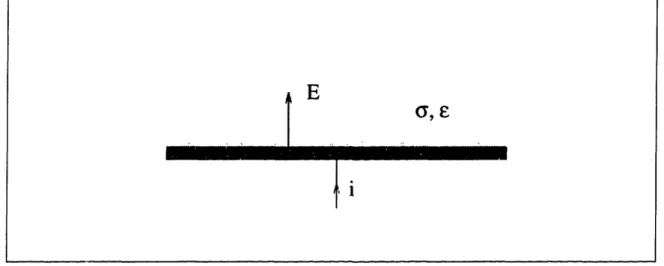
1-1 Terminal current of an electrode in contact with a conducting dielectric

medium ... 16

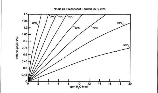
1-2 An illustration of the manner in which the real part of the complex permittivity is made up of contributions from all loss processes [1, pp. 50] 20 1-3 Equilibrium relationship between the moisture content of transformer oil and pressboard for temperatures ranging from 20°C to 90°C . . . 22

1-4 Imposed w-k dielectrometry ... 23

2-1 Structure of the parallel-plate sensor ... 27

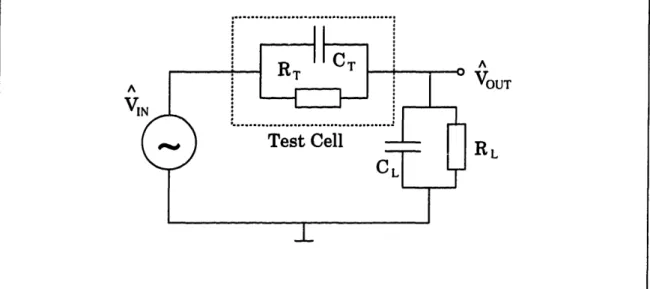
2-2 Equivalent circuit of the test structure ... 28

2-3 Relative dielectric constant of Teflon measured with the parallel-plate sensor ... 33

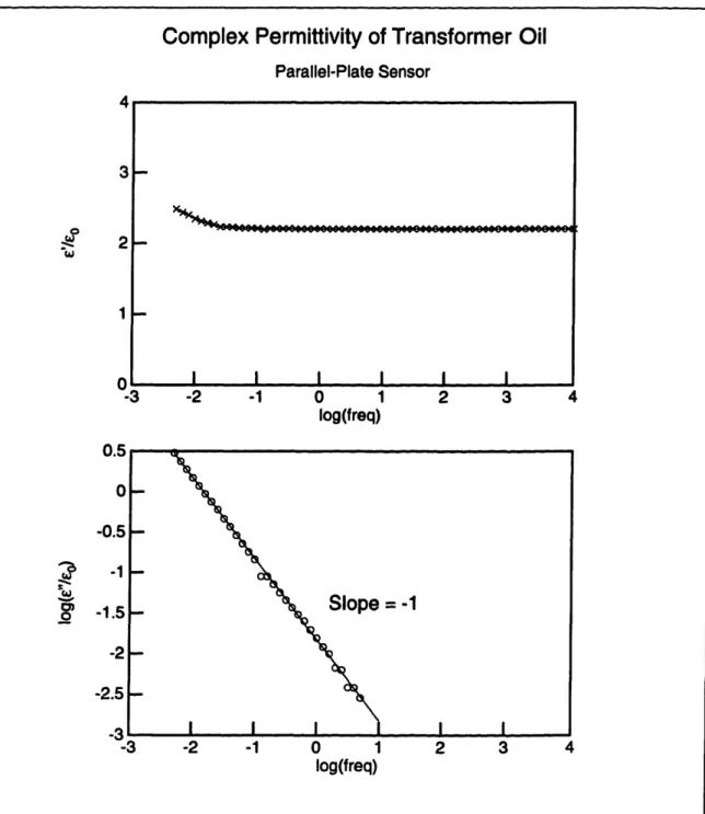
2-4 Complex permittivity of transformer oil measured with the parallel-plate sensor ... 34

2-5 Sensitivity of the inversion formulas to noise ... 36

2-6 Temperature transient ... 40

2-7 Pressboard conditioning transient ... . 42

2-8 Raw gain-phase data for a frequency scan of a representative press-board sample ... 44

2-9 Dielectric spectrum of a representative pressboard sample ... 45

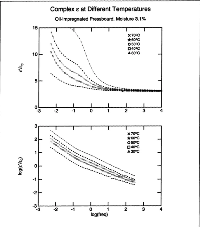
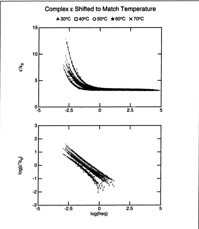
2-10 Dielectric spectra of a pressboard sample (MA) at five temperatures . 49 2-11 Universal curve for one sample (MA) at five temperatures ... 50

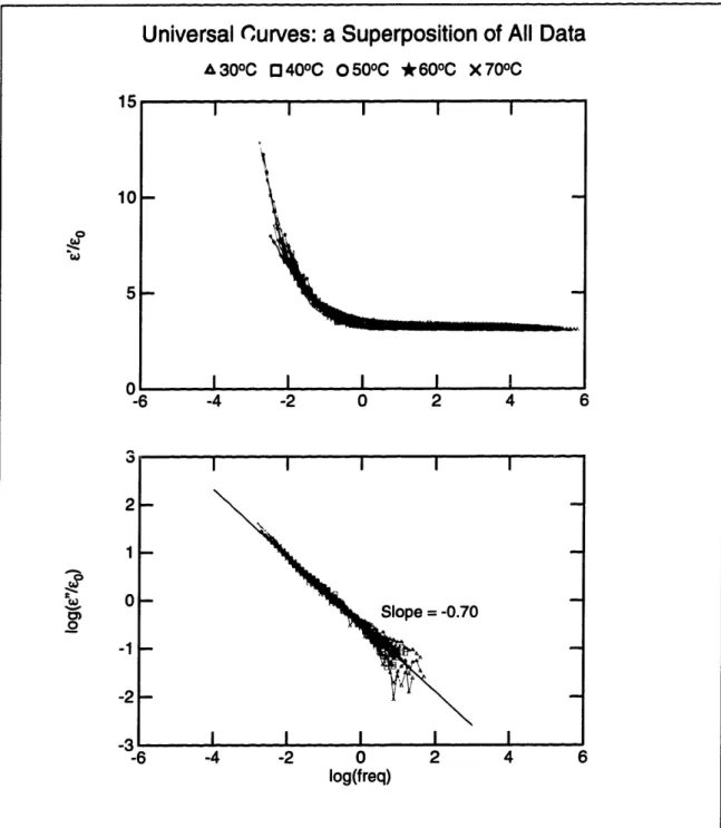
2-13 Temperature-shifted families of curves for the seven samples, each of the families being a universal spectrum for that sample ... 52 2-14 Master Universal Spectrum, containing data from 35 frequency scans,

shifted with moisture and temperature ... 53

2-15 Logarithmic frequency shift as a function of temperature ... 56 2-16 Logarithmic frequency shift as a function of temperature: Arrhenius plot 57

2-17 Logarithmic frequency shift as a function of moisture ... 57

3-1 Structure of the three-wavelength interdigitated sensor [2] ... 61 3-2 Mask used for the copper back plane deposition ... 62

3-3 Response of a three-wavelength sensor in air before chemical cleaning and before Parylene coating ... 65 3-4 Response of a three-wavelength sensor in air before Parylene coating

and after recommended chemical cleaning procedure and heating . . . 66

3-5 Interdigitated electrode structure with a number of homogeneous layers above it ... 67

3-6 Lumped circuit model for the interdigitated sensor structure ... 69

3-7 A representative layer of homogeneous material ... 71 3-8 Piecewise-smooth collocation-point approximation to the potential

be-tween the electrodes of an interdigitated structure ... 74

3-9 A frequency scan of the Parylene coated three-wavelength sensor in air 77

3-10 Raw gain-phase data of the three-wavelength sensor in Shell Diala A transformer oil ... 79

3-11 Dielectric spectrum of Shell Diala A transformer oil taken with the

three-wavelength sensor ... ... 80

4-1 Stair-step approximation of a dielectric profile with the marching

ap-proach ... 90

4-2 Solutions to the diffusion equation at different values of normalized timel04

4-3 Curve fitting of equation 4.44 to the data representing the frequency shift as a function of moisture ... 105

5-1 Experimental setup for profile measurements taken with the 3-A sensor 110 5-2 Dielectric spectra of oil-free pressboard under vacuum ... 111 5-3 Gain-phase data taken with the three-wavelength sensor on polymers 113 5-4 Permittivity of polymer structure as calculated from every wavelength

of the three-wavelength sensor . . . 114

5-5 Dielectric spectrum of oil-impregnated 0.25 mm Crocker paper at room

temperature . . . ... 117

5-6 Raw gain-phase data taken with the three-wavelength sensor on

sixteen-ply Crocker paper . . . ... 119

5-7 Dielectric spectra taken with the three-wavelength sensor on Crocker

paper ... 120

5-8 Dielectric spectra of oil-impregnated Crocker paper drying under vac-uum, taken with the 5.0 mm wavelength of the three-wavelength sensor 122 5-9 Dielectric spectra of oil-impregnated Crocker paper drying under

vac-uum, taken with the 2.5 mm wavelength of the three-wavelength sensor 123 5-10 Dielectric spectra of oil-impregnated Crocker paper drying under

vac-uum, taken with the 1.0 mm wavelength of the three-wavelength sensor 124 5-11 Permittivity and conductivity of Crocker paper adjacent to the

three-wavelength sensor, calculated by the multidimensional algorithm at 0.01 Hz, as a function of time ... 125 A-1 A Hilbert transform pair satisfying the Kramers-Kr6nig relations . . . 135 B-1 Reliability of water vaporizer measurements as a function of oven

tem-perature ... 138

B-2 Reliability of water vaporizer measurements as a function of sample thickness ... 140

B-3 Reliability of water vaporizer measurements as a function of oven

tem-perature ... 142

E-1 Interface box circuit diagram ... 152 E-2 Results from measurements of the load impedance of the parallel-plate

sensor's interface box ... 153

List of Tables

1.1 Diffusion coefficients of water in transformer oil and pressboard [2] . . 21

2.1 Impregnation process parameters for the pressboard samples used in

the universal spectrum ... 38

2.2 Moisture Measurements for the pressboard samples used in the univer-sal spectrum ... 39

2.3 Relative logarithmic frequency shifts for data at different temperatures

and moisture contents ... 54

2.4 Logarithmic frequency shift due to temperature ... 55 2.5 Logarithmic frequency shift due to moisture content ... 55

3.1 Values of parameters describing the three-wavelength sensor [2] ... . 61

4.1 Computation time of program est.c as a function of initial guess and solution using multidimensional estimation ... 95 4.2 Effect of noise on the results from the multidimensional parameter

estimation ... 96

4.3 Computation time versus frequency of Jacobian updates for est.c . . 96

4.4 Computation time of program ests.c as a function of initial guess and solution using the simplex method ... . 99

5.1 Layer structure for polymer experiment ... 112 5.2 Poor results of applying the root-finding multidimensional parameter

5.3 Results from applying the root-finding multidimensional algorithm to

Crocker paper data at 0.01 Hz ... 118

5.4 Results of applying the multidimensional parameter estimation algo-rithm to data at 0.01 Hz taken after the application of vacuum to oil-impregnated Crocker Paper ... 121

D.1 Summary of Controller Commands ... 149

E.1 Interface Box Load Impedances ... .. 154

G.1 Summary of data processing software ... 159

Chapter 1

Introduction

1.1 Motivation

In this thesis we discuss dielectrometry measurements of insulating materials, with an emphasis on solid and liquid transformer insulation, and their application to the

measurement of the moisture content of these materials.

Monitoring the condition of the insulation is of particular importance to high-power transformers, where the insulating materials are subjected to high levels of

electrical and thermal stress.

1.1.1 High Power Transformers

High-power transformers are an essential element in the distribution of electrical en-ergy. The demand for energy is perpetually increasing, placing ever tougher require-ments on the performance characteristics of these transformers. The transmission of greater quantities of electrical energy affects the operation of the transformers by requiring efficient transmission of more energy at higher voltages, which in turn sub-jects transformer insulation to higher levels of electrical stress. In addition, the heat dissipation due to losses in the transformer cores and windings requires higher coolant speeds, which in turn increases the level of static electrification.

tion of high-power transformers, because they have been pushed to their limits, which is reflected in the increase of transformer failures. The need for greater efficiency has reduced the margin of safety in the operation of the transformers, making it very important to identify and predict critical conditions that may lead to failures.

The presence of moisture in the solid and liquid transformer insulation, i.e. press-boa d and oil, is a major factor that affects the operation of the transformers. Al-though moisture does not seem to greatly affect the conductivity of the oil, it reduces

its dielectric strength. Moisture also affects the conductivity of the pressboard, which in turn increases the dissipated power and the rate of static charge relaxation, which

is a crucial factor in static electrification phenomena.

Load transients which transformers undergo, especially upon power-up, cause

rapid changes in the insulation's temperature. Temperature affects the solubility equilibrium of moisture between the solid and liquid insulation and also directly influences the insulation's conductivity. Moisture in the oil may under decreasing temperature transients result in free water that can lead to electrical breakdown. A

mass transfer process of water results from the equilibrium imbalance, in which at higher temperatures moisture leaves the pressboard to enter the oil. The oil

estab-lishes moisture equilibrium with an interfacial zone at the surface of the pressboard.

The steady state is reached when moisture from deep inside the pressboard diffuses to the surface to establish a uniform moisture distribution. The transient interfacial dry zones are highly insulating, and as a consequence significant surface charge can

accumulate to cause surface spark discharges. Such critical conditions can lead to a

high level of static electrification and possibly catastrophic failure of the unit. It is therefore important to be able to monitor the moisture dynamics in such systems, in

order to understand the failure mechanisms and to prevent critical conditions.

1.1.2 Other Applications

The dielectrometry methods developed specifically for pressboard have applications in many other fields also: The dielectric properties of a material are greatly affected

Figure 1-1: Terminal current of an electrode in contact with a conducting dielectric medium

stress, etc. In polymers, the dielectric constant may be related to the degree of polymerization. There are many applications in quality control, where deviations in

the dielectric properties of a material may correspond to flaws in its structure.

As materials age, their dielectric constant and conductivity may change too. In

general, whenever the condition of a dielectric material must be monitored, dielec-trometry measurements provide a simple, non-destructive, real-time measurement,

which can be related to the property in question.

1.2 Dielectric Properties of Materials

There are two parameters of a medium that determine the quasi-static distribution

of electric fields: the dielectric permittivity and the conductivity . The former determines the displacement current density from the electric field, while the latter

relates the conduction current density to the electric field. The permittivity governs

energy storage (reactive power) phenomena, while the conductivity determines the power dissipation (active power).

Consider an electrode in contact with a medium as shown in Figure 1-1. Since

the total current density due to conduction and displacement is in the same direction

(,

£

i

__

one-dimensional geometry of Figure 1-1, the current densities and the electric field

are perpendicular to the electrode. Let the electric field at the electrode surface be E.

We are interested in the total terminal current per unit electrode area J that flows into the electrode. Integrated over the electrode area, this would yield the terminal

current:

i

=j

The component of J due to conduction follows the ohmic constitutive law:

J,= aE

(1.2)

Jd_ d = (cE) (1.3)

dt dt

The total terminal current per unit electrode area is then:

d

J =

J

+

Jd= aE + (E)

(1.4)

If the system is under AC steady-state operation, every quantity F(t) may be expressed as:

F(x,y, z,t) = {P((, y, z)ejwt} (1.5) where w is the radian frequency of excitation. If e is constant with time, we may

rewrite equation 1.3 in terms of complex amplitudes as:

Jd

=

jweE

_(1.6)

For the total current density we may then write:

It is convenient to define the complex permittivity e of a medium as:

e =

E- je"

a--

(1.8)

which lets us rewrite equation 1.7 in a form similar to equation 1.6, thus combining conduction phenomena with polarization phenomena:

J = jw*E

(1.9)

We shall use this definition of the complex permittivity throughout this thesis.

1.2.1 Dielectric Spectra

The dielectric spectrum of a material is a representation of its complex permittivity,

f* = ' - j", as a function of frequency. The real component ' gives the dielectric constant while the imaginary component d" determines the power dissipation (loss)

in the material.

Once it is known how the dielectric spectrum of oil-impregnated pressboard varies with temperature and moisture, it is possible to measure the moisture content in a sample by taking a frequency scan and comparing the results to the known calibration mapping. This type of mapping is unique to every type of paper and may depend on the amount of impurities in it. Such a mapping for pressboard is presented in Chapter 2.

1.2.2 Kramers-Kronig Relations

The Kramers-Kr6nig relations link the real and imaginary components of the disper-sive part of the complex permittivity, defined in equation 1.8. As a direct consequence of causality, the following equations hold:

x

1 pf+0o X'(x) dx

"(w)

=

p

X()dz

(1.11)

71 00-o X--W

where the real and imaginary parts of the dispersive part of the dielectric susceptibility

X* are defined as follows:

I _{= e= CoX'+ EC' (1.12)}

I

=

-=

OX"+

aO

(1.13)

* = x' - ix

(1.14)

Appendix A presents the derivation of these relations and some of their consequences.

In this section we discuss what the Kramers-Kr6nig relations can tell us about the dielectric spectra of materials.

In an ohmic material, and a are independent of the frequency or amplitude of the applied electric field and a plot of log('"/Eo) versus logw has a slope of -1. As

discussed in Appendix A, for such materials X* = 0.

In a dispersive material. when e" is plotted against frequency on a log-log scale, it can be characterized by one or more loss peaks. The magnitude of the slope at

which these peaks are approached on either side is between 0 and 1 for most mate-rials [1, pp. 163-200]. For every loss peak in the e" spectrum, there is an associated

elevation in the ' spectrum proportional to the area under the corresponding peak in e" [1, pp. 47-52]. This is illustrated in Figure 1-2.

1.3 Moisture Dynamic Processes in

Pressboard/Oil Systems

Section 1.1.1 discussed the significance of the presence of moisture in solid and liquid transformer insulation. During thermal transients complex dynamic processes

Figure 1-2: An illustration of the manner in which the real part of the complex permittivity is made up of contributions from all loss processes [1, pp. 50]

equilibrium of the system, causing the initiation of moisture mass transfer processes. Transformer oil and pressboard are very dissimilar materials, in that the former is

hydrophobic and the latter is hydrophilic. Typical values for the water content of pressboard are 0.5-5%, while in oil at room temperature the saturation moisture

con-tent is about 50 ppm (parts per million). As a consequence, almost all of the moisture present in the system resides in the pressboard. As the temperature changes moisture

will move into or out of the pressboard via diffusion.

1.3.1

Diffusion

The rate of diffusion of moisture through the oil and the pressboard determines the

time rates of change of the moisture distribution, and thus how long it takes before

equilibrium is reached. Experiments have determined the diffusion constants of water

in these two media to have the values shown in Table 1.1 [2].

In order to appreciate the magnitude of these diffusion constants, we can calculate that the diffusion times of water across A = 1 mm of pressboard, given by

OiX

Diffusion coefficient Symboll Value at 15°C

I

in pressboard Dp 6.7 x 10-14 m2/s 6.0 x 10-12 m2_/s

Table 1.1: Diffusion coefficients of water in transformer oil and pressboard [2] are half a year and two days at 15°C and 70°C respectively. What that means is that equilibrium is generally never reached in an operating transformer, given how quickly

the oil temperature changes with the power load and the ambient air temperature. Instead, oil equilibrates only with a thin layer of pressboard at its surface. This implies that the surface of the pressboard may become extremely dry, which could lead to

static charge accumulation and partial discharges, ultimately leading to catastrophic failure.

1.3.2

Equilibrium

The equilibrium of moisture between the oil and the pressboard is what determines the direction of the mass transfer processes in the pressboard/oil system. This equilibrium is extremely sensitive to temperature, as can be seen in Figure 1-3. This is how a temperature transient drives the system our of equilibrium and initiates the mass transfer processes. If, for example, the moisture concentration in the paper is 0.5%, at 20°G, the oil humidity in equilibrium with it is about 0.5 ppm. If the oil temperature then changes to 800C, the new equilibrium value for the oil humidity becomes close to 6.5 ppm, i.e. thirteen times higher, which would drive water out of the pressboard surface and leave it very dry until moisture deep in the pressboard diffuses to the

surface on a time scale of order r in equation 1.15.

1.4 Imposed w-k Dielectrometry

The simplest way to measure the complex permittivity of a material is to place it

between parallel electrodes and then measure its complex impedance. This is the idea behind the parallel-plate sensor described in Section 2.1. In that case the electric fields

Norris Oil-Pressboard Equilibrium Curves

Figure 1-3: Equilibrium relationship between the moisture content of transformer oil and pressboard for temperatures ranging from 200C to 90°C

are uniform and independent of position in space. If instead the two electrodes are placed side by side only on one surface of the material, the electric fields will decrease away from the electrodes and the complex impedance between the two electrodes will be most sensitive to the material adjacent to them. The disadvantage of this two-dimensional method is that the problem of calculating the impedance as a function of the material's complex permittivity is much more complicated.

The idea of placing both electrodes on the same surface is at the base of the method of imposed w-k dielectrometry. The two electrodes are shaped as a multitude

of interdigitated fingers, as shown in Figure 1-4. The electric fields are uniform in the z-direction and periodic in the y-direction with a spatial wavelength of A. Thus at every surface of constant x the electric potential is periodic in y and can be expanded as an infinite series of sinusoidal Fourier modes of spatial wavelengths A,, = A/n. This

is very convenient, because the solutions to Laplace's equation

1.3 1. 1.0 0. . 0.7 O. 0.4 0. 0.1 ppm H20 in oil .,

Figure 1-4: Imposed w-k dielectrometry

in Cartesian geometry are of the form

= o0 hyp(kx) trig(ky) (1.17)

where hyp(x) stands for any one of the hyperbolic exponential functions sinh(x), cosh(x), eo, or e-m, and trig(x) stands for one of the trigonometric functions sin(x) or

cos(x;). For every Fourier mode n, the electric fields decrease with x as exp(-2irnx/A)

with the fundamental mode n = 1 penetrating farthest into the material.

By designing sensors with various spatial wavelengths A, it is possible to test the

dielectric properties of materials at different depths. Combining the results from

several such sensors makes it possible to determine the x-dependent spatial profiles

of the complex permittivity.

The three-wavelength sensor, described in detail in Chapter 3, uses the ideas presented in this section. Section 3.3 in that chapter develops the mathematical

model of the interdigitated sensors.

1.5 Scope of Thesis

In this thesis we present the several stages of research that lead to the ultimate goal of studying the dynamics of mass transfer processes in pressboard/oil systems by

measuring moisture profiles.

First, we establish a relationship between the moisture content of pressboard and its complex permittivity. In this way we can convert dielectric profiles into moisture

profiles. Chapter 2 presents the methods used in the establishment of this relationship. The next step is to introduce spatially dependent dielectrometry measurements, which provide information about the spatial variation of the complex permittivity.

Such sensors are the interdigital sensors. Chapter 3 presents the construction and

modeling of the interdigital sensors in general, with specific emphasis on the three-wavelength sensor, which is a hybrid sensor capable of taking measurements at three distinct spatial wavelengths simultaneously.

Chapter 4 discusses the various issues associated with the interpretation of data from the interdigitated sensors. It also presents in detail several numerical algorithms

which are used for the interpretation of such data and the establishment of spatial profiles.

Finally, in Chapter 5 we present the results from the application of the concepts developed in the previous three chapters to actual measurements with the three-wavelength sensor. Future work may include applying the entire methodology

es-tablished in this thesis to monitoring and studying of the mass transfer processes of

water in a simulated transformer environment.

In addition to presenting new concepts and results from experiments and theoret-ical work in the subject of interdigital dielectrometry, this document is also meant

to serve as a reference for those who are interested in continuing the work presented

in the implementation of the various numerical procedures and in the process of data acquisition and interpretation. Familiarity with references [3] and [2] would prove to be very helpful to the reader of this document.

Chapter 2

Features of the Dielectric

Spectrum of Pressboard

2.1 Parallel Plate Sensor

The simplest way to measure the permittivity and the conductivity of a material is to place it between a pair of parallel plates of known area and separation, thus

producing a lossy capacitor. This test cell can be modeled as a resistor in parallel with a capacitor. The complex admittance of the structure can then be measured,

and from there its permittivity and conductivity can be calculated.

We have used this simple idea in the development of the parallel-plate sensor. Its structure is shown in Figure 2-1. The figure shows more than just a pair of conducting plates. The actual capacitive structure is comprised of the driven electrode

and the sensing electrode. Underneath the sensing electrode lies the guard electrode.

The guard electrode is driven by a buffer amplifier stage to be always at the same

potential as the sensing electrode. The buffer amplifier is situated in the interface

box, described in detail in Appendix E. The sensing electrode is also surrounded by a ring electrode, which is connected to the guard electrode. In addition to shielding the

sensing electrode from external electric fields, the guard electrode serves to eliminate

Parallel-Plate Sensor

Driven Electrode

Pressboard Sample

Teflon Spacer

.

Sensing Electrode

Ground Electrode

duminum

?ressboard

Teflon

Figure 2-1: Structure of the parallel-plate sensor

multiplied by the gain of the operational amplifier, making their effects negligible. Although the guard electrode is driven by a much lower impedance source as com-pared to the sensing electrode, namely the operational amplifier, it is still necessary

to shield it from outside fields, and that is the purpose of the ground electrode. A triaxial cable is used to connect the sensor to the interface box. The center conductor

is connected to the sensing electrode, the middle - to the guard electrode, and the outer - to ground. The ideas about shielding, as discussed above, are fully

applica-ble to the connecting triaxial caapplica-ble too. The driving voltage is applied via a separate coaxial cable.

Another advantage to having a guard ring around the sensing electrode is that the

electric field is highly uniform and there are essentially no fringing fields associated with that electrode. The material sample is larger in area than the sensing electrode,

thus letting all field lines terminating on it pass through the material sample. Teflon

was chosen as the insulating material between the different electrodes because of its excellent thermal properties in addition to being a very good insulator. The entire

- --

-~~~~~~~~~~~~~~ A VOUT RL A VI

Figure 2-2: Equivalent circuit of the test structure

'sandwich' structure is tightened together with insulating nylon bolts.

2.1.1

Circuit Model

As shown in Appendix E, the input admittance of the interface box, with which the sensing electrode is loaded, is that of a known parallel RC-pair. Therefore the test structure relevant to the measurement may be modeled as shown in Figure 2-2.

The following equations relate the test-cell lumped parameters RT and CT (see

Figure 2-2):

d

RT = A (2.1)

EA

CT = d (2.2)

where d is the plate separation distance, A is the sensing electrode area, and l and e

are the material's conductivity and permittivity respectively. Equations 2.1 and 2.2 make it clear that the geometry of the test cell may be described by a single parameter,

the capacitance of the structure in air (CAIR):

CAIR = d (2.3)

d

which is an easily measured parameter. In terms of equation 2.3, we have:

RT = Co (2.4)

OCAIR

CT = CAIR (2.5)

Co

For linear time-invariant (LTI) systems we take the standard form:

VIN = R{VINe°' (2.6)

VOUT = R{VOUTe"} (2.7)

with E'IN and VfOUT defined in Figure 2-2. The controller, described in Appendix D is

responsible for generating the driving voltage and measuring the output voltage. The data that it produces is expressed in terms of a magnitude 20log(M) [dB] and phase

'np 180/7r [deg], which are related to the complex amplitudes defined in Figure 2-2 in

the following way:

IM I |U (2.8)

VIN

= L f j (2.9)

Y VIN

/

Since the values of M and 'p are needed as defined above, as opposed to the way

they are presented by the controller (i.e. in dB and deg), they need to be transformed

to that form first. The symbol L used in equation 2.9 is defined as:

Lz = tan-1 2{z} (2.10) RIZI)

for a complex number z.

The next step in calculating a and e is to calculate RT and CT from measurements of M and y, and the known values of RL and CL. We define the admittances of the

test and load branches as YT = 1/RT + sCT and YL = 1/RL + sCL respectively, where

s is the complex frequency. Then from the voltage divider relationship we obtain:

VOUT YT R + _{SCT CT s +}

RT (2.11)

VIN

with the zero z and the pole p located at:

z= - 1 (2.12)

RTCT

- (1 1

CL)

Depending on the values of RT, CT, RL, and CL, either of z and p may be larger than

the other. In the limiting case of s -+ 0, the voltage ratio becomes real and equal to

RLI(RL + RT). In the other extreme, where s - oo, the voltage ratio is also real and

equal to

In our work we drove the system at the sinusoidal steady state, so that s = jw.

Then

Vo UT YT

V

Me

_(2.14)

VIN Y + YL

YT

Mej'

M cos + jM sin p

YL

1-Mej'-

1-Mcos p-jMsin

(M cos o + jM sin )(1 - M cos

y

1 + M2 cos2 P - 2M cos + M2sin2 y

{ YT } M cos

y(1

M

sin

YL

1 + M

- 2Mcosp

1 + M

_-

_2Mcos

₍

4 {YT

M sin

sin

M sin

(217)

From the definitions of YT and YL we obtain

R + jWCT = YT

+ jWCL)

(2.18)

RT YL /L

and from there

1 Mcosp-M (- Msin (wCL) (2.19) RT 1 + M2-

2Mcos

RL

+

1+M2 2Mcoso

RL)+ + M

Mcos(CL)

(

RT

M

(2.21)

where

C

e of a material from gain and phase data recorded by the controller.

If it is necessary to calculate RL and CL based on knowledge of RT and CT, which

occurs if we want to measure the load impedance of an interface box by replacing the test cell with a known test impedance, then the formulas take up the following form:

RL = RT (2.23)

cos - M + sin p

C

os - M - (1/C) sin

=

(2.24)

M

which is particularly useful for diagnostics of interface boxes (see Appendix E). The program testrc.c uses these formulas.

This inversion process is carried out by the program inv.c, listed in Section G.4, which takes as an input the raw output file generated by the controller box, and

outputs values for e' = e and e" = a/w in files with extensions .el and .e2 respectively.

The program reads the setup file .invsetup, also listed in Section G.4, which contains the default values for CAIR, CL, and RL. An alternative setup file may be given as

an argument.

2.1.2 Testing

In order to test the performance of the parallel-plate sensor, we used it on known materials, in particular Teflon and transformer oil. Figure 2-3 shows the gain and phase of the measurement on Teflon. Only /e0 is shown, because a was too low to measure. In the figure the average measured value of e, the relative dielectric

constant, is e/e0o = 2.1, which is exactly the value quoted in the literature [4]. There is no variation with frequency over the range of 0.005-10,000 Hz, which is consistent with the known non-dispersive properties of Teflon.

Shell Diala A transformer oil was used in the oil experiment. Figure 2-4 shows the results. On a log-log scale, the plot of e" versus frequency is a straight line of

slope -1, which means that a is independent of the frequency. This is characteristic of an ohmic material. For linear dielectric materials, ' should also be constant with

frequency. The observed rise of e' at the lower end of the frequency range can be attributed to double layer formation at the aluminum-oil interface [2]. This plot

corresponds to o = 0.83 x 10-12 U/m and e/eo = 2.2, which are typical values for the dielectric parameters of this kind of transformer oil.

The plot of e" is not shown for frequencies higher than 100.7 Hz. This is because at

that frequency range the response is fully dominated by the capacitive element, and

no meaningful information about the conductivity may be inferred. This insensitivity of the response to the conductivity is discussed in more detail the next subsection.

2.1.3 Measurement Sensitivities to the Load Impedance

Looking at the circuit in Figure 2-2 it is immediately obvious that when w - oo

and w -, 0 the response will be fully dominated by the capacitors or the resistors

respectively. In those two extreme cases the complex amplitude ratio is purely real,

Dielectric Constant of Teflon Parallel-plate sensor -2 -1 0 1 log(freq) 2 3 4 Figure 2-3: sensor

Relative dielectric constant of Teflon measured with the parallel-plate

-1 -2' -3' 'o. ._

0

Complex Permittivity of Transformer Oil Parallel-Plate Sensor 3 0 w 2 1 n s1 n 2"_W

9

Figure 2-4: Complex permittivity of transformer oil measured with the parallel-plate sensor

__

III I Il II II

--- I~~·AA LL~~llW-·Y -- l1y

· · ii · iii · · · 3 'A m IL_ I I I _I_ t

which extreme the frequency is. There is a special case, namely RT/RL = CL/CT,

when V = 0 for every w. From a strictly mathematical point of view, this special case is the only case when V is exactly zero. This is why these equations "assume" when given = 0 that this special case holds.

In reality, of course, we are limited by the precision of the equipment, and therefore it is impossible to measure resistances reliably above a certain frequency. It is similarly impossible to obtain reliable estimates for the capacitances below a certain frequency. Since we have some flexibility in choosing RL and CL, we should like to choose such values that our measurements of RT and CT would be most reliable. This is the topic of this section.

Equations 2.12 and 2.13 define the zero and the pole of the system, which roughly delimit the interval of frequencies for which both RT and CT can be reliably estimated. Somewhere between these two frequencies, t0 reaches an extremum, before returning to zero again (see Figure 2-5). If the pole frequency is lower than the zero frequency,

p is always negative, and if the pole is at a higher frequency, than the zero to is always

positive. We would like to place the peak (or trough) of V close to the center of the interval of frequencies in which we are most interested. This is how we came up with the values of RL = 9.8 GfS and CL = 120 pF shown in Figure E-1.

So far the discussion of sensitivity has been qualitative. In order to quantify these considerations, we go on to calculate the sensitivities of the estimated values for RT and CT. We define the sensitivity of a quantity y with respect to a quantity as

follows:

SY = l'O-. (2.25)

The sensitivity describes what the relative change in y would be for a change in z. If G and p are the magnitude and phase of the response expressed in dB and deg respectively, related to M and p as follows,

G = 20 log M (2.26)

180

= -180 (2.27)

Inversion Process Sensitivities RT = 160 Gi RL = 9.8 Gil CT = 35.2 pF CL=120 pF 00oo 0 0 0 0 0 0 0 0 0 OXXX_XXx x x x 0 x 0 0 0 0 0 0 00 _o x o -2 -1 0 1 x 0 X o 00 0 0 I 1Cb 2 -2 -1 0 log(freq) 1 2 3

Figure 2-5: Sensitivity of the inversion formulas to noise. The bottom plot shows the dependence of the logarithm of S and S with frequency. These sensitivities show how much a and /i would change for a small change in p. These ratios are least sensitive to noise for low values of S and SO

-5 :' C X -10 -15 -20 40 30

0

x

and we make the additional definitions

RL

Mcos cp

(2.28)

CT M cos tp - M2_{+ (1/C)M sin}

_(2.29)

tCh

-

1 + M

_{- 2Mcos}

_p

then we obtain the following equations for the sensitivities of a and P/ with respect to G and p:

Oa dM

(1 + M

)cos - 2M - C(1 - M

)sinpV Mln 10

S _

=

Sa

o8a dop M{(M 2 - 1)sinp - [(M 2 + 1)cos 0- 2M]} r

S

=

-

.

(2.31)

SP

i

S.3

_9O

dM _ (1 + M

)cos

2M+(1/)(1 - M

)sinp Mln10

(2.32)

G-AM dG (1 + M2- 2Mcosp)2 _{20/ (}

8a:3 dp M{(M 2 - 1)sin + (1/C)[(M 2 + 1)cos p - 2M]} r (2.33)

s =

.' dp

=

" ;I dp (1 + M2 - 2M cos) 2 180,8

Figure 2-5 shows gain G and phase p as a function of frequency. It also shows log ISp I and log IS0I. One can see that a and

/3,

2.2 Experimental Procedures

The objective of this set of experiments is to study how the dielectric spectrum of oil-impregnated pressboard changes with variations in temperature and moisture content.

The dielectric spectrum is to be measured with the parallel-plate sensor, described in detail in Section 2.1.

We first prepared many samples of pressboard, each with a different content of

water. We then measured the moisture content of a sample, placed it in the sensor structure, scanned its dielectric spectrum at five different temperatures and finally

Vacuum Drying Oil Immersion

Sample Temperature Duration Vacuum Temperature Duration

Name [0C] [hours] [mTorr] [°C] [minutes]

NB 70 12 25 5 x 105 ND 70 24 70 60 MA 70 10 300 70 10 MB 70 2/3 400 60 10 MC 70 1/3 550 70 10 MD 70 2 200 70 10 MF 70 4 160 70 10 MG 70 15.5 100 70 10

Table 2.1: Impregnation process parameters for the pressboard samples used in the universal spectrum

2.2.1

Impregnation

The equipment used to impregnate our samples of pressboard with transformer oil is described in detail in Appendix C. Prior to impregnation we cut 50 mmx50 mm pieces of 1 mm thick oil-free EHV-Weidmann HIVAL pressboard. Then we placed them in the impregnation chamber, one at a time, for various lengths of time, in

order to obtain different moisture contents. Table 2.1 lists the parameters of the

oil-impregnation process that every sample underwent.

2.2.2

Moisture Measurements

The moisture of each sample was measured before and after it was placed in the

parallel-plate sensor with the help of the Mitsubishi VA-05 water vaporizer and the

Mitsubishi CA-05 moisture meter. The use of this equipment is described in Ap-pendix B. That apAp-pendix also discusses the need to split the pressboard samples into

many thin layers before depositing in the vaporizer oven, a procedure strictly followed in this set of measurements.

We define the moisture content of pressboard as the weight of water liberated

. NB ND MAI MB IMCI MD MF MG

Moisture 3.1

1

Table 2.2: Moisture Measurements for the pressboard samples used in the universal

spectrum

oven. Since this kind of moisture measurement was destructive, in that the sample cannot be used after it has been in the vaporizer, in order to measure the moisture

content of a pressboard sample, we cut off small pieces of it.

If the two moisture measurements were not close to each other, the data of the sample was not used. This happened for samples NA, NC, aPr ME. Table 2.2 lists the average results of the moisture measurements.

2.2.3 Temperature Transients and Control

Measurements with every sample were taken at five temperatures: 300C, 40°C, 50°C, 60°C, and 70°C. The parallel-plate sensor, with the pressboard sample placed inside it, is placed in an oven, whose temperature is controlled by a feedback temperature

controller. We could not go above 70°C because of the temperature limitations of the connecting triaxial cable. A small fan inside the oven made sure that the air is well

stirred, so that there would be no temperature gradients inside the volume.

Following a change in the temperature setting, the oven temperature undergoes a

transient, whose characteristics are determined by the temperature controller

param-eters and the thermal inertia of the oven. The temperature of the sample itself lags a bit behind the temperature of the oven. In order to determine when the sample has

reached the required temperature, we measured the complex impedance of a sample at a single frequency (in order to make the measurement time short) about ten times

an hour for four hours after stepping the oven setting from 250C to 500C. We have

lost record of the frequency at which this measurement was performed, although it

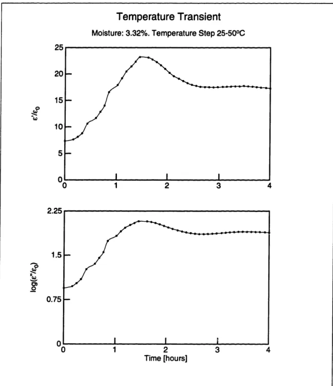
lies in the range 0.01-0.1 Hz. This poses no problem, since the only significance of the frequency is to ensure that e" can be reliably measured. The results from this measurement are shown in Figure 2-6. The high measured values of E' and e" are due

Temperature Transient

Moisture: 3.32%. Temperature Step 25-50°C

w

w

0o

0

Time [hours]

Figure 2-6: Transient in complex permittivity of a pressboard sample in response to

to low frequency dispersion. We concluded that we must wait for about four hours after we change the temperature setting before taking a frequency scan. The high values of ' are due to low-frequency dispersion in pressboard (see Section 2.3).

2.2.4

Conditioning

We have observed that in addition to the short (4 hours) temperature transient, the complex permittivity of a sample experiences another, long transient. When we tested

a sample for 270 hours at a constant temperature (500°C) we observed the behavior illustrated in Figure 2-7. The long time constant of this transient suggested that it may be due to mass transfer processes of water in the pressboard. Since the sample in

the test cell is sealed from the outside air, and since diffusion of water through 6 mm of pressboard before it reaches the active area would require months', we concluded that this sample conditioning process is probably due to moisture redistribution within the

bulk of the pressboard, finally resulting in a uniform distribution.

We then established the rule that after a sample is impregnated and placed in

the test cell, we must let it stay there for at least five days (120 hours) before any measurements are performed. This period of time for the sample to reach moisture equilibrium is necessary only once. Once it expires, only the four hours discussed in

the previous section are required for the sample to reach thermal equilibrium after a temperature setting change.

2.3 Results

We would like to establish a relationship between the temperature and moisture content of pressboard, and its dielectric spectrum. This can be accomplished by

1Based on values for the diffusion constant taken from [2, Table 5.3], namely Dp = 5.8 x

10-12m2/s at 700C and 6.3 x 10-14m2/s at 150C.

d2

r = - = 36 days to 18 years D,

Conditioning Transient of Oil-Impregnated Pressboard Temperature 50°C 100 Moisture 0.860% 200 Time [hours]

Figure 2-7: Pressboard conditioning transient

0 4

0

summarizing the results from frequency scans taken at several different moisture

contents and temperatures.

2.3.1 Features of a Representative Dielectric Spectrum

Figure 2-8 shows the raw gain-phase data of a frequency scan of an oil-impregnated pressboard sample taken with the parallel-plate sensor. The offset data serves to check whether an unreasonably high voltage has built up at the input of the operational amplifier due to leakage currents, which could cause amplifier saturation. The mea-sured gain and phase curves show a lot of similarity with the computer-generated ones

in Figure 2-5. There are, however, some differences: One can see in Figure 2-8 that the breakpoint of the voltage ratio magnitude is at approximately 10-0° 8 = 0.16 Hz. This breakpoint occurs 3dB up from the pole defined in equation 2.13, which for our experiment is to the right of the zero. Past the pole, as w - oo, the gain

contin-ues to change (it decays with a very slight negative slope), which is not the case in Figure 2-5. This is because the permittivity and conductivity of pressboard change with frequency, while the computer-generated data assumed constant RT and CT. This difference is due to the dispersive nature of pressboard which alters the shape

of the curves somewhat. An ohmic material would manifest behavior similar to that

in Figure 2-5.

The dispersive nature of the pressboard does not affect the validity of

Equa-tions 2.21 and 2.22, since they are evaluated at a single frequency. If we process the data shown in Figure 2-8 to produce values for the complex permittivity, we obtain

the results shown in Figure 2-9. This processing of data is done with the help of the

program inv.c, listed in Section G.4.

The first thing to note in Figure 2-9 is that all e" data for frequencies above about

10 Hz is noise. As explained in Section 2.1.3, this is due to the lack of sensitivity at

high frequencies of the measurement to the resistive component of the material. When we disregard this data, the rest of the e" points lie approximately on a straight line.

This line does not have a slope of -1, characteristic of an ohmic material. Instead, the slope is approximately -0.7. This comes to confirm the previous observation that

Raw Gain-Phase-Offset Data Sample MA at 500C -2 -1 0 1 log(freq) 2 3 -3 -2 -1 0 1 2 3 4 log(freq) X X X XX XX x ) x X xX- -- Xx ' Xx x xx

~x

Figure 2-8: Raw gain-phase data for a frequency scan of a representative pressboard sample 0 -5 -10 C .co (5 O) a Cu a. I I I I I I -15 -20 42 -35 28 21 14 7 O _ >dO x_X x X x x

I

II -x

I--

Dielectric Spectrum Sample MA at 500C 6 o 3 0 O) 0 -2 -1 0 1 log(freq) 2 3 4 -3 -2 -1 0 1 2 3 4 log(freq)

Figure 2-9: Dielectric spectrum of a representative pressboard sample

I I I I I I

f%

S

the material is dispersive.

This decay of " is associated with a loss peak, as described in Section 1.2.2.

However, the actual peak is not visible in Figure 2-9, because it occurs at a frequency which is below our bottom limit (0.005 Hz). The elevation in c', which accompanies

a loss peak in e" (see Section 1.2.2), is clearly shown at the top of the figure.

All but one of the pressboard samples studied displayed very similar behavior.

One sample, NB, which had the highest moisture content (3.1%) is a bit different. Its dielectric spectrum is shown in Figure 2-12 and discussed in Subsection 2.3.2.

2.3.2

Frequency Shift Algorithm

Often the shape of the loss peaks in the dielectric spectrum of a material are indepen-dent of moisture and temperature. They only shift position. It should therefore be possible to create a single universal spectrum, to which all other spectra map, after

having been shifted (horizontally with frequency and/or vertically) by an amount which is a function of the temperature and moisture content [5] [6].

In this case, if there is only one loss peak, the entire spectrum could be described

by the position of a single point, namely the peak itself, with coordinates (p, CE). If there are two or more peaks, and their relative position does not change (which is

required if the shape is to remain constant), then a point of inflection could be chosen as the reference point [6].

Appendix A proves that a shift in either c' or e", both horizontally and vertically,

must be accompanied by an identical shift in the other component of c*. This is required by the Kramers-Kroinig Relations (Section 1.2.2). A linear scale for ' is chosen in Figure 2-9 for reasons of clarity. If, however, c, (the permittivity at infinite

frequency) were to be subtracted from ', then plotted on a log-log scale ' would also

be a straight line with the same slope as e". See Appendix A for a discussion of this corollary of the Kramers-Kr6nig Relations.

It is unfortunate that the loss peak occurs at such low frequencies, because a

shift the spectra either only horizontally, only vertically, or in some combination. We have chosen to move only horizontally, as suggested by research done elsewhere [6].

Since these shifts are relative, any spectrum may be chosen as the reference. The amount of shifting required to map a spectrum to the reference should be determined by some "best-fit" rule, such as a least-squares fit. If we need to find a best fit of a function f(pl 2, ... ,pn, ), where pi are the unknown parameters, to a reference

function g(x) over an interval E [a, b] by the least-squares method, we must first find the error function:

e(Pl,P2,... ,n) =j [f(PlIP2, ... pn X ) g(X)]2d (2.34)

and then solve the system of n simultaneous equations:

de

-= 0,

for i=1, 2,...,n

(2.35)

api

However, fitting straight lines presents the difficulty that the slope is already known and there is only one unknown parameter, the intercept. If the slopes are slightly different, then the two lines will not overlap perfectly and there will be no best fit on an interval of (-oo,oo), because the integral in equation 2.34 does not

exist. On a closed interval the method outlined above will place the line in a way that it crosses the other line close to the midpoint of the interval, but we do not consider this fit to be the "best fit" of a line to another line.

For these reasons we have chosen a numerical method, implemented in the program fith.c (Appendix G). It attempts to fit the two spectra by trying shifts in increments of 0.1 (on a logarithmic scale), because this is the frequency resolution of the controller (see Appendix D). It numerically finds the shift that minimizes the sum of the squares of the differences between the corresponding points. The results of the application of this algorithm to the data collected with the parallel-plate sensor are discussed in