response of electrochemical cells
The MIT Faculty has made this article openly available.
Please share
how this access benefits you. Your story matters.
Citation
van Soestbergen, M., P.M. Biescheuvel, and M.Z. Bazant.
"Diffuse-charge effects on the transient response of electrochemical cells."
Physical Review E 81.2 (2010): 021503. © 2010 The American
Physical Society
As Published
http://dx.doi.org/10.1103/PhysRevE.81.021503
Publisher
American Physical Society
Version
Final published version
Citable link
http://hdl.handle.net/1721.1/58745
Terms of Use
Article is made available in accordance with the publisher's
policy and may be subject to US copyright law. Please refer to the
publisher's site for terms of use.
Diffuse-charge effects on the transient response of electrochemical cells
M. van Soestbergen,1,2P. M. Biesheuvel,3and M. Z. Bazant4
1
Materials Innovation Institute, Mekelweg 2, 2628 CD Delft, The Netherlands 2
Department of Precision and Microsystems Engineering, Delft University of Technology, Mekelweg 2, 2628 CD Delft, The Netherlands 3
Department of Environmental Technology, Wageningen University, Bomenweg 2, 6703 HD Wageningen, The Netherlands 4Department of Chemical Engineering and Department of Mathematics, Massachusetts Institute of Technology, Cambridge, Massachusetts
02139, USA
共Received 27 October 2009; published 12 February 2010兲
We present theoretical models for the time-dependent voltage of an electrochemical cell in response to a current step, including effects of diffuse charge共or “space charge”兲 near the electrodes on Faradaic reaction kinetics. The full model is based on the classical Poisson-Nernst-Planck equations with generalized Frumkin-Butler-Volmer boundary conditions to describe electron-transfer reactions across the Stern layer at the elec-trode surface. In practical situations, diffuse charge is confined to thin diffuse layers 共DLs兲, which poses numerical difficulties for the full model but allows simplification by asymptotic analysis. For a thin quasi-equilibrium DL, we derive effective boundary conditions on the quasi-neutral bulk electrolyte at the diffusion time scale, valid up to the transition time, where the bulk concentration vanishes due to diffusion limitation. We integrate the thin-DL problem analytically to obtain a set of algebraic equations, whose共numerical兲 solution compares favorably to the full model. In the Gouy-Chapman and Helmholtz limits, where the Stern layer is thin or thick compared to the DL, respectively, we derive simple analytical formulas for the cell voltage versus time. The full model also describes the fast initial capacitive charging of the DLs and superlimiting currents beyond the transition time, where the DL expands to a transient non-equilibrium structure. We extend the well-known Sand equation for the transition time to include all values of the superlimiting current beyond the diffusion-limiting current.
DOI:10.1103/PhysRevE.81.021503 PACS number共s兲: 82.45.⫺h
I. INTRODUCTION
Time-dependent models for electrochemical cells are widely used in science and technology. In the field of power sources, the charge/discharge cycle of batteries关1–5兴 and the
startup behavior of fuel cells关6兴 are important topics.
Time-dependent models with electrochemical reactions have been used to describe, e.g., light-emitting devices关7兴, metal
depo-sition in nanotubes 关8兴, ion intercalation in nanoparticles
关9,10兴, corrosion 关11兴, ion-exchange membranes 关12兴, and
electrokinetic micropumps关13,14兴.
Sand’s classical theory 关15兴 of the transient voltage of a
flat electrode in response to a current step is based on a similarity solution of the diffusion equation in a semi-infinite, one-dimensional domain with a constant-flux bound-ary condition 关16兴. Experimental data from
chronopotenti-ometry of electrochemical cells 关16兴 and galvanostatic
intermittent titration of rechargeable batteries 关2兴 are
rou-tinely fitted to Sand’s formula, but discrepancies can arise because the theory assumes linear response in a neutral bulk solution and ignores diffuse charge near the electrodes. Charge relaxation in a thin diffuse layer 共DL兲 can be in-cluded empirically by placing a capacitor in parallel with the Faradaic current 关16,17兴 or more systematically, by
analyz-ing the underlyanalyz-ing transport equations, which has been ex-tensively developed for blocking, ideally polarizable elec-trodes关18–22兴. For nonblocking electrodes passing Faradaic
current, these approaches must be extended to include the Frumkin correction and other nonlinear modifications of the reaction rate associated with diffuse charge关23兴.
The usual starting point to describe the transport of ions is the Poisson-Nernst-Planck共PNP兲 theory, which leads to a set of coupled nonlinear differential equations. These equations
are difficult to solve numerically due to the formation of local space-charge regions near the electrodes, typically in very thin DLs whose width is on the order of the Debye screening length 共⬃1–100 nm兲. Within the DLs, gradients in concentration and electrical potential are very steep, com-pared to gradual variations in the quasi-neutral bulk electro-lyte at the scale of the feature size of the system, often orders of magnitude larger. In numerical models this would lead to the requirement of a very fine spacing of grid points near the electrodes, especially in two and three dimensions 关24兴. To
circumvent this problem a vast amount of previous work assumes electroneutrality throughout the complete electro-lyte phase, thus neglecting the DLs关3–6,16,25,26兴. The DLs,
however, cannot be neglected as they influence the charge-transfer rate at the electrodes and make a significant contri-bution to the cell voltage关23,27–34兴.
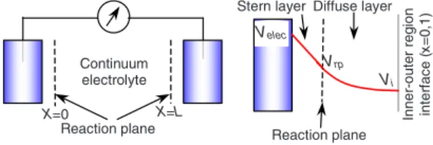
To describe Faradaic reaction rates at the electrodes, it is reasonable to assume that the charge transfer occurs at some atomic distance away from the electrodes, at the “reaction plane”共for an atomically flat electrode兲, which serves as the edge of the continuum region representing the electrolyte 共Fig. 1兲. The reaction plane is commonly equated with the
“outer Helmholtz plane” or “Stern plane” of closest approach of solvated ions to the surface, so the electrolyte region is separated from the electrode by a thin Stern monolayer of solvent molecules on the electrode 关35兴. The Stern layer is
often viewed as uncharged and polarizable with a reduced dielectric constant compared to the bulk, due to dipole align-ment in the large normal field of the DL. This model, which we adopt below, neglects specific adsorption of ions, which break free of solvation and adsorb onto the surface at the “inner Helmholtz plane” within the Stern layer, either as an intermediate step in Faradaic reactions or without any charge
transfer. In that case, the electrolyte is effectively separated from the electrode by a thin dielectric coating, the Stern layer, and we postulate that electron-transfer reactions occur across this layer, biased by the local voltage drop关27兴. More
sophisticated models of the DL are available, including vari-ous models with finite-sized ions and solvent molecules, as reviewed in Ref.关14兴. Even the simplest approach used here,
however, provides a rich microscopic description of Faradaic reactions at the electrode surface that goes well beyond the standard approach in electrochemistry of applying the Butler-Volmer equation across the entire double layer 关16兴,
i.e., across both the DL and Stern layer 共without the “Frumkin correction”关23,27兴兲.
Regardless of the detailed model of the Stern layer, its local potential drop, which biases electron tunneling and Faradaic reaction rates, has a complicated nonlinear depen-dence on the accumulated charge and voltage across the DL. In order to complete the model, an electrostatic boundary condition is required at the Stern plane, which we take to be a Robin-type condition equating the normal electric field with the Stern layer voltage, effectively assuming a constant field in the Stern layer关23,28,30,31兴. Combining this
bound-ary condition self-consistently with Butler-Volmer kinetics for the charge-transfer reaction, biased by the Stern voltage, leads to a unified microscopic model, which we refer to as the “generalized Frumkin-Butler-Volmer” 共gFBV兲 equation 关23,27–34兴 共see Ref. 关23兴 for a historical review兲. In our
work, the gFBV equation is beneficial over the traditionally used Butler-Volmer equation since it provides a natural boundary condition for the full PNP theory, including diffuse charge关23,30,31兴.
In the current work we develop a simple semi-analytical theory of the time-dependent response of an electrochemical cell with thin DLs共compared to geometrical features of the cell兲 and validate it against numerical solutions of the full PNP-gFBV equations. The simple model circumvents the nu-merical problems in solving the full model by using matched asymptotic expansions to integrate across the DL to derive effective boundary conditions on the quasi-neutral bulk solu-tion. We focus on the typical situation where the neutral salt concentration just outside the thin DL remains non-negligible 共prior to diffusion limitation兲, in which case the diffuse charge profile of the DL remains in quasi-equilibrium 关21–23,30–34,36–42兴, even while passing a significant 共but
below limiting兲 current. Time-dependent breakdown of quasi-equilibrium and concomitant expansion of the DL has
just begun to be analyzed for blocking electrodes关18,21兴, but
this is a major complication for electrochemical cells passing Faradaic current, which to our knowledge has only been ana-lyzed in steady-state situations关32兴.
The thin-DL model extends classical time-dependent models based on the hypothesis of electroneutrality through-out the complete electrolyte phase, by treating reaction kinet-ics at the electrodes in a self-consistent way, properly ac-counting for diffuse charge 共i.e., accounting for the DLs兲. The effective equations and boundary conditions of the thin-DL model are very general and can be applied to any transient problem, but we illustrate their use in the standard case of a suddenly applied, constant current between parallel-plate electrodes. Unlike transient problems involving a suddenly applied voltage across parallel plates 关18–20兴 or
around a metallic particle or microstructure 关39,40,43兴,
which involve nontrivial, time-dependent coupling of the DL and quasi-neutral bulk regions, the situation of one-dimensional transient conduction at constant current offers a well-known analytical simplification, namely, the salt con-centration of the quasi-neutral bulk evolves according to the diffusion equation 共Fick’s law兲 with constant flux boundary conditions due to mass transfer at the electrodes关18,44–50兴,
while the time evolution of the DLs共and thus the total volt-age of the cell兲 is slaved to that of the bulk concentration. The bulk diffusion problem has an exact solution in terms of an infinite series关46–49兴, which describes the spreading and
collision of diffusion layers from the two electrodes. Prior to collision of the diffusion layers 共and prior to the transition time discussed below兲, the solution can also be approximated more accurately by similarity solutions for semi-infinite do-mains near each electrode关14,15兴. These classical solutions
are used to infer the mass transfer properties of an electrolyte from experimental transient measurements 关51–53兴.
In our analysis, we neglect the very early stage of tran-sient response, where first the bulk region and later the double layers charge capacitively, prior to the onset of bulk diffusion. During charging of the double layers, the bulk con-centration remains nearly uniform, and thus the bulk acts such as a resistor in series with the double layer capacitors. The associated “RC” time scale can be expressed asDL/D,
where D is the electrolyte diffusivity, L is the electrode spac-ing, and D is the Debye screening length, which sets the thickness of the diffuse double layers 关18兴. At low voltages
or in the absence of Faradaic reactions, this is the relevant time scale for transient response, e.g., in high-frequency im-pedance spectroscopy experiments 关36,54,55兴 or
induced-charge electrokinetics, where high-frequency alternating cur-rents are applied 关13,38–40兴. The bulk diffusion time scale
L2/D, which is much larger than the RC time for thin DLs
共by a factor of L/D兲, becomes important in presence of
Faradaic reactions关23,30–33兴 or at large applied voltages for
blocking electrodes where the DL adsorbs neutral salt such that the bulk region becomes depleted 关18,21,22,38兴. In this
work we will focus on the diffusion time scale, as we are interested in the start-up behavior of electrochemical cells at longer times than the relaxation time, all the way up to the steady-state. Consequently, the transient solutions we present here can be regarded as an extension into the time-dependent domain of the steady-state solutions reported previously in Refs. 关23,31,32兴. Continuum electrolyte X=L X=0 Reaction plane Velec Vi Inner-out e r reg ion int er fa c e (x =0 ,1 ) Diffuse layer Stern layer Vrp Reaction plane
FIG. 1.共Color online兲 Schematics of the electrochemical cell. In the simplified model the continuum electrolyte is split in an outer 共bulk兲 and inner 共diffuse layer兲 region, the latter present on both electrodes. The potential in the electrode 共Velec兲 decays linearly across the Stern layer to the reaction plane共Vrp兲 and decays further
To show the accuracy of the simplified approach for thin DLs we will compare results with full model predictions and show that they compare very favorably for all parameter set-tings that we investigate, except for very short time scales where the relaxation time scale applies. Furthermore, we will show results for the classical transition time, or “Sand’s time,” when the salt concentration approaches zero at either electrode due to an applied current exceeding diffusion limi-tation 关16,46,56兴. For such large currents, we show that the
cell potential reaches an infinite value for the thin-DL limit, while it remains finite for any nonzero DL thickness, due to the expansion of the DL into a different non-equilibrium structure. Analogous effects, first studied in the context of overlimiting direct currents in electrodialysis 关57兴, have
re-cently been analyzed for steady-state problems involving Faradaic reactions关31,32兴 and for time-dependent problems
involving large ac voltages with blocking electrodes关21兴, but
we are not aware of any prior modeling of the transient re-sponse to an overlimiting current in electrochemical cells with Faradaic reactions.
II. THEORY
In this section we will discuss a time-dependent model for a planar one-dimensional electrochemical cell containing a binary electrolyte, i.e., the electrolyte contains only two spe-cies, namely, cations, at a concentration Cc共X,t兲, and anions, at concentration Ca共X,t兲. The continuum electrolyte phase is
bounded by the two reaction planes共one on each electrode兲, where we assume that the only reaction is the formation 共at the anode兲 or removal 共at the cathode兲 of the cations 共Fig.1兲.
The anion is assumed to be inert and as a result the total number of anions in the system is conserved; no such num-ber constraint applies for the reactive cations. This situation describes, for example, an electrolytic cell with metal depo-sition at the cathode and dissolution at the anode, or a gal-vanic cell, such as a proton exchange membrane共PEM兲 fuel cell conducting protons across a membrane, or a thin-film Li-ion battery shuttling Li+between intercalation electrodes.
The charge-free Stern layer is located in between the reaction planes and the electrodes, and is treated mathematically via the boundary conditions.
In the full PNP model the electrolyte phase is modeled by the same set of equations thoughout the entire electrolyte phase, all the way up to the reaction planes, irrespective of the amount of local charge separation 共which is low in the bulk and high near the reaction planes兲. However, in the simplified model that we will discuss, the continuum electro-lyte phase is divided in two domains. The first domain is the outer region where electroneutrality can be assumed, a re-gion which we will also refer to as the bulk rere-gion. The second domain is the inner region共found on both electrodes兲 where we have a nonzero space-charge density such that it captures the DLs. We will first present the full model for ion transport and the electrochemical reactions based on the full PNP-gFBV theory, from which we derive the simplified, semi-analytical, model using the singular perturbation theory. For both models we will focus on the situation where a con-stant current is prescribed and we will follow the
develop-ment of the cell potential as function of time. A. PNP-gFBV theory
To describe ion transport in the electrolyte phase, the Nernst-Planck共NP兲 equation is the standard model, in which it is assumed that ions are ideal point charges.共For a review of more general, modified NP equations for concentrated electrolytes with finite-sized ions, see Ref. 关14兴.兲 In this
work, we also neglect convection fluxes of ions, due to flow of the solvent. In this case the NP equation combined with a mass balance, leads to
C˙i= −XJi=X关Di·共XCi+ zi· Ci· f ·XV兲兴, 共1兲
where C˙iis the time derivative of the ion concentration Ci, Ji
is the ion flux, Di is the ion diffusion coefficient, zi is the valence of the ions, V is the local electrostatic potential in volts, f equals e/kBT, with e as the elementary charge, kBis
Boltzmann’s constant, and T is the temperature. The sub-script i either denotes the reactive cations, i.e., c, or the inert anions, i.e., a. In Eq. 共1兲, X is the spatial coordinate which
runs from the first reaction plane at X = 0 to the second reac-tion plane at X = L共Fig.1兲 and thus applies up to the plane of
closest approach for both the cations and anions, irrespective of whether the ion is inert or electrochemically reactive. In the local-density mean-field approximation, the mean elec-trostatic potential is related to the charge density by Pois-son’s equation, X 2 V = − e
兺
i ziCi, 共2兲where is the dielectric permittivity. If we combine Eqs. 共1兲
and共2兲 we obtain the full PNP theory.
The flux of cations at the reaction planes due to the elec-trochemical reaction of these ions to a metal atom共or other reductant species兲 in the electrode 共Me兲 can be described by the gFBV equation关23,27–34兴,
JF= KRCOexp共−␣R· f⌬VS兲 − KOCRexp共␣O· f⌬VS兲, 共3兲
where ⌬VS is the potential drop across the Stern layer
共⌬VS= Velec− Vrp, see Fig.1兲, Kiare kinetic constants, and␣i
are the transfer coefficients共here␣i=12 is assumed关31兴兲; the
subscripts O and R denote the oxidized state 共or oxidation reaction兲 and reduced state 共reduction reaction兲, respectively. In the present work we consider that the ion is converted to a neutral metal atom and incorporated in the electrode 共and vice versa兲, i.e., Cc+ e−↔Me. Therefore we can assume a
constant metal atom concentration 共reduced state兲, so from this point onward we can make the replacement
JO= CRKOfor a constant oxidation reaction rate.
Next we discuss the dimensionless parameters that are applicable to Eqs. 共1兲–共3兲 and which we will use in the
re-mainder of this work, following Refs. 关18,21,23,30–32,39,41兴. First we have the dimensionless
electrostatic potential, = f · V, the average total concentra-tion of ions, c =共Cc+ Ca兲/共2C⬁兲, and diffuse charge density,
=共Cc− Ca兲/共2C⬁兲, where C⬁is the initial average ion con-centration, set by the ionic strength of the bulk electrolyte.
Note that the average ion concentration is only constant for the anions, but not necessarily for the cations, due to the absence of a constraint on equal formation and removal rates, which can lead to nonzero total charge in the electrolyte 共balanced by opposite charges on the electrodes兲 关23,30–32兴.
These two rates become equal only when the steady-state is reached, while in the time up to the steady-state an excess or deficit of reactive ions is produced. Further, we introduce the length scale x = X/L. At this length scale, the Debye length, D=
冑
kBT/2e2C⬁, becomes ⑀=D/L. Next, we scale theStern layer thickness to the Debye length such that its dimen-sionless equivalent becomes ␦=s/D. We scale time to the
diffusion time scale discussed above, so the dimensionless time is = tD/L2. Note that here we implicitly assume that the diffusion coefficient of both ionic species are equal and are independent of the ion concentration. Finally, we scale the ion flux to the diffusion-limiting current,
j = Ji/Jlim= JiL/4DC⬁, such that the dimensionless kinetic constants of the gFBV equation become kR= KRC⬁/Jlimand
jO= JO/Jlim.
Making these substitutions, the PNP equations take the dimensionless form c˙ =x共xc +x兲, 共4a兲 ˙ =x共x+ cx兲, 共4b兲 ⑀2 x 2= −. 共4c兲
The boundary conditions that apply at the reaction planes for the transport equations are given by
xc +x= − 2jF, 共5a兲 x+ cx= − 2jF, 共5b兲
where the Faradaic rate of formation共or removal兲 of cations at the reaction planes is given by
⫾ jF= kR共c +兲exp
共
− 12⌬S
兲
− jOexp共
12⌬S
兲
, 共6兲where the ⫾ sign refers to the positive value at position
x = 1 and the negative value at position x = 0. Note that we
define a flux of cations from x = 0 to x = 1 as positive. The potential drop across the Stern layer equals the po-tential in the adjacent metal phase,elec, minus the potential at the reaction plane, rp, and relates to the electrical field
strength at the reaction plane according to关23,30–32兴
⌬S= ⫾ ⑀␦·x, 共7兲
where the ⫾ sign again refers to the positive value at posi-tion x = 1 and the negative value at posiposi-tion x = 0. The bound-ary conditions for the Poisson equation can be determined as follows, namely, by making use of the fact that in the elec-trolyte the imposed electrical current i is equal to the sum of the ionic conduction current and the Maxwell displacement current 关11,30兴. This equality is generally valid at each time
and each position. At the electrodes, the ionic conduction current is also always exactly equal to the Faradaic 共i.e., electrochemical or charge transfer兲 reaction rate, jF. The con-duction current in the electrolyte results from the migration
of ions, with initially both the cations and anions contribut-ing to this current, while at the steady-state only the flux of cations remains. The Maxwell current共which, dimensionally, is −xV˙ 兲 originates from changes with respect to time of the
electrical field strength, and thus vanishes at steady-state. As a result we have关11,12,30,36兴 i = −1 2共x+ cx兲 − 1 2⑀ 2d dx, 共8兲
for the current in the electrolyte phase, which becomes
i = jF−1 2⑀
2d
dx, 共9兲
at the reaction planes. Instead of using Eq. 共9兲 directly, we
integrate and use关11,12兴
x= 2 ⑀2
冕
0 关⫾ jF共⬘
兲 − i兴d⬘
, 共10兲for the electrical field strength, x, at the reaction planes.
We will refer to the set of equations described above as the full PNP model.
B. Thin-DL limit
Next, we use singular perturbation theory 共matched asymptotic expansions兲 to simplify the full PNP model by integrating across the DLs to obtain a set of equations and effective boundary conditions for the quasi-neutral bulk re-gion, which is more tractable for numerical or analytical so-lution. In the case of transient one-dimensional response to a constant current between parallel plates, we will see that the thin-DL model can be solved analytically, at least in implicit algebraic form. This well-known approach provides a sys-tematic mathematical basis for the physical intuition that the problem can be solved in two distinct domains, namely, the “inner region” of the DLs and “outer region” of the quasi-neutral bulk solution 共Fig. 1兲 and appropriately matched to
construct uniformly valid approximations, in the asymptotic limit ⑀→0 of thin DLs compared to the system size 关18,30–33,37,58兴.
We first discuss the inner solution, describing the structure of the DLs, which are present at both electrodes. The inner regions are defined by the coordinate system y = x/⑀for the region near x = 0 and y =共1−x兲/⑀ for the region near x = 1. Conversion of Eq.共9兲 to inner coordinates results in the fact
that the Maxwell current will vanish for ⑀→0 共thin-DL limit兲. Consequently, the Faradaic current becomes equal to the current imposed on the system, i.e., jF=⫾i. Then we can
eliminate c +at the reaction plane from Eq.共6兲 as described
next. Namely, we substitute Eq. 共4c兲 in Eq. 共4a兲, convert to
the inner coordinates and perform the integration with the matching conditionsy=y2= 0 for y→⬁, which yields
c =12共y兲2+ ci, 共11兲
for the variation across the inner region of the concentration
c 共note again, only for the condition that ⑀→0兲, where ci
Next, we substitute Eq. 共4c兲 into Eq. 共4b兲, rewrite and
con-vert to the inner region coordinates, then substitute Eq.共11兲
and finally perform the integration with the matching condi-tions,y=y
3= 0 for y→⬁, to obtain y3−
1
2共y兲3− ciy= 0, 共12兲
for the thin-DL limit. Equation共12兲 is identical to the
steady-state Smyrl-Newman master equation 关30,32,33,37兴
con-verted to the inner coordinate system for ⑀→0, cf. Bonne-font et al. 关30兴. Consequently, as for the steady-state, it is
possible to derive from Eq.共12兲 the classical approximation
that the DLs are in quasi-equilibrium共with a Boltzmann dis-tribution for a dilute solution兲 in the asymptotic limit
⑀→0 关30–33,37,45兴, even in the presence of a nonzero
nor-mal current, until the nearby bulk salt concentration reaches very small O共⑀2/3兲 values. We will not show this derivation
here as it is carried out in detail by Bonnefont et al.关30兴. At
larger currents共beyond the transition time discussed below兲, the double layer loses its quasi-equilibrium structure 关37兴,
and matched asymptotic expansions for overlimiting currents at Faradaic electrodes关32兴 or ion-exchange membranes 关58兴
have revealed a more complicated nested boundary-layer structure for the DLs, including an intermediate non-equilibrium extended space-charge layer.
In this work, we only consider the asymptotic limit of thin quasi-equilibrium DLs, such that an infinite voltage would be required to surpass the diffusion-limited current and force the DL out of equilibrium. In this common situation, we can relate c + at the inner-outer region interface to c + at the reaction plane using the Boltzmann distribution for ions as ideal point charges关23,30,34兴,
crp+rp= ciexp共− ⌬DL兲, 共13兲
where the subscript rp refers to the reaction plane and ⌬DL=rp−i, which is the potential drop across the DL
from the reaction plane, rp, to the inner-outer region
inter-face,i共Fig.1兲. Note that in Eq. 共13兲 we implicitly assume = 0 in the outer region as Eq. 共4c兲 vanishes there for
⑀→0. Next, we can use the Gouy-Chapman theory to
deter-mine the potential drop across the Stern layer according to 关23,30,34兴
⌬S= 2
冑
ci␦sinh共
12⌬DL
兲
, 共14兲which is again valid when the DLs are in quasi-equilibrium and follows from Eq. 共12兲 as described in Ref. 关30兴. Note
that the dimensionless Stern layer thickness ␦ depends on the ion concentration via the Debye screening length D⬀1/
冑
ci. In Eq.共14兲 we use冑
cito correct␦ for anyvaria-tions in the Debye length due to variavaria-tions of the ion con-centration at the inner-outer region interface 关23兴. Although
Eqs.共13兲 and 共14兲 are equilibrium properties of the DL, they
have also proven to be very useful in describing the steady-state current of electrochemical cells关23,30–33兴, for the
rea-sons giving above. For thin DLs, there is no direct effect of the Faradaic current on the concentration profiles near the electrodes at leading order in the asymptotic limit 苸→0 when considering the inner region coordinate system 关30–33兴. Nevertheless, the magnitude of the potential drop
across the Stern layer, and thus across the DL, is indirectly influenced by the Faradaic current via the gFBV equation and Stern boundary condition. Next, we can substitute Eqs. 共13兲 and 共14兲 into Eq. 共6兲, which concludes the mathematical
description of the two inner regions. Finally, we require the concentration, ci, at the inner-outer region interface
共match-ing condition兲, which we will explain next.
To determine the concentration at the inner-outer interface we require the outer region solution. For ⑀→0 it follows from Eq. 共4c兲 that the space-charge density vanishes
throughout the complete outer region. As a result the deri-vates of the space charge with respect to time, ˙ , and the
spatial coordinate, x, will vanish as well. Consequently,
Eq. 共4b兲 will vanish and Eq. 共4a兲 results in the linear
diffu-sion equation, c˙ =x
2
c 关41,42,44–50兴, which is
mathemati-cally equivalent to Fick’s second law for the diffusion of neutral particles 关48,59兴. The same diffusion equation
also applies here to the bulk salt concentration,
c =共Cc+ Ca兲/共2C⬁兲, at leading order, thus recovering the
classical model for a neutral electrolyte关16,45,59兴. 共For
un-equal diffusivities in a neutral binary electrolyte, the associated bulk salt diffusion coefficient is the “ambipolar diffusivity” 关45兴.兲 The corresponding boundary conditions
are given by Eq.共5a兲, which also simplify due to the
vanish-ing space-charge density in the outer region for ⑀→0; namely, they become xc = −2jF. The ability to replace the
full PNP equations in the bulk of the cell by Fick’s law for diffusion is an important simplification from the thin-DL limit since the number of unknown fields is reduced from three to one in the outer region. Namely, we solve for the concentration c, which is the unknown field variable, while equals zero and the potential drop across the outer region can be determined from an algebraic equation as discussed be-low. Furthermore, we can make use of various exact solu-tions to the diffusion equation in one dimension for various types of boundary conditions.
In this work, we apply a constant current to a cell with planar electrodes, as explained above. Note that for⑀→0 the second term in Eq.共9兲, i.e., the Maxwell term vanishes such
that jF=⫾i. With these assumptions, the diffusion equation
has an exact solution in terms of an infinite series 关48,49兴
共which can be systematically derived, e.g., by finite Fourier transform 关59兴兲,
c共x,兲 = 1 + 2i
再
12− x −
兺
n=1n=⬁
关fncos共2Nx兲兴
冎
, 共15兲where fn= exp共−4N2兲/N2 and N =1
2共2n−1兲, a solution
which has been applied to model the transient current in electrochemical cells for at least a century on the basis of electroneutrality throughout the complete electrolyte phase 关46,47,50兴. Here we apply Eq. 共15兲 in a model which
con-siders space-charge regions and Stern layers as well. Due to the applied current we have either an injection or removal of salt at the edges of the outer region resulting in gradual variations of the salt concentration, which are ini-tially localized near the edges of the outer region in the so-called diffusion layer. Equation 共15兲 describes the spreading
it can be truncated at a small number of terms in the long-time limit 共Ⰷ1兲. Eventually, the exponential term in Eq. 共15兲 vanishes when →⬁, leaving c共x兲=1+i共1–2x兲, which
is exactly the classical steady-state solution for planar elec-trochemical cells关3,23,30–33兴. Note that the steady-state
so-lution is physically valid 共with positive concentration at the cathode兲 only below the diffusion-limited current, i.e., i⬍1. Larger transient currents are possible, but lead to vanishing salt concentration at the “transition time” discussed below.
For early times, prior to collision of the diffusion layers, the series in Eq. 共15兲 converges very slowly, and it is more
accurate to use similarity solutions for semi-infinite diffusion layers. Close to each electrode, the bulk concentration is well approximated by the classical solution to the diffusion equa-tion in a semi-infinite domain with a constant-flux boundary condition 关14,15兴. In order to construct a uniformly valid
approximation for early times, we add two such similarity solutions to the initial constant concentration, one at the an-ode for an enrichment layer and one at the cathan-ode for a depletion layer, resulting in
c共x,兲 = 1 + 4i
冑
·再
ierfc冉
x2
冑
冊
− ierfc冉
1 − x2
冑
冊
冎
, 共16兲 where ierfc共x兲=1/冑
exp共−x2兲−x erfc共x兲 关see Fig.5共b兲兴. Wefocus on the early time regime below when analyzing the transition time and proceed to use the series solution for more typical situations below the limiting current.
We can now use the set of Eqs. 共6兲 and 共13兲–共15兲 under
the condition that jF=⫾i to solve for the potential drop
across the DL and Stern layer, as function of time and im-posed current. The potential drop across the outer region for
⑀→0 follows from Eq. 共8兲 by integration, namely,
⌬outer=
冕
x=0
x=1 2i
c共x,兲dx, 共17兲
where c共x,兲 follows from either Eq. 共15兲 or 共16兲. In
deriv-ing Eq. 共17兲 we make use of the vanishing space-charge
density,, as mentioned previously. Furthermore, in Eq.共17兲
the term 2/c共x,兲 can be regarded as a local Ohmic resis-tance for the outer region. For the steady-state we can use
c共x兲=1+i共1−2x兲 in Eq. 共17兲 and obtain the classical result
⌬outer= 2 tanh−1共i兲 关3,23,30–33兴. Finally, we can define the
potential drop across the complete system, i.e., the cell po-tential, as
cell=关⌬S+⌬DL兴x=0+⌬outer−关⌬S+⌬DL兴x=1. 共18兲
We can now solve Eqs. 共6兲, 共13兲–共15兲, 共17兲, and 共18兲 as a
small set of nonlinear algebraic equations to describe the dynamic problem in case of the limit of⑀→0, which we will refer to as the thin-DL limit.
C. GC- and H-limits
Analytical solutions for the voltage against current curve for the steady-state have been presented in literature for two limits based on the Stern boundary condition, namely, the Gouy-Chapman 共GC兲 limit ␦→0 and the Helmholtz 共H兲 limit ␦→⬁ 关23,31兴. In the GC-limit, the reaction plane
co-incides with the electrode surface and the Stern layer does not sustain any voltage drop. For this limit we can derive the potential drop across the DL directly from Eq.共6兲,
substitut-ing Eq. 共13兲 and ⌬S= 0, such that we obtain
⌬DL,GC= ln
冉
kR,mci,m
jO,m⫿ i
冊
, 共19兲
where ci,m is the concentration at the inner-outer region in-terface and subscript m either denotes the anode 共A兲 at x=0 or the cathode 共C兲 at x=1. In the GC-limit the effect of a nonzero space-charge density in the DL is at maximum due to the absence of the potential drop across the Stern layer. In contrast, in the opposite H-limit this effect completely van-ishes as the potential drop in this case is completely across the Stern layer, i.e., we assume an infinite Stern layer thick-ness relative to the thickthick-ness of the DL. Consequently, the H-limit coincides with models based on electroneutrality, where zero space-charge density is assumed for the complete electrolyte phase 关23兴. The potential drop across the Stern
layer in the H-limit can be derived from Eq.共6兲 if we assume
that the reaction plane coincides with the inner-outer region interface such that
⌬S,H= 2 ln
冉
⫾i +
冑
i2+ 4jO,mkR,mci,m2jO,m
冊
. 共20兲 The concentration ci,mcan be determined by either
substitut-ing x = 0 or x = 1 into Eq. 共15兲, which yields
ci共兲 = ⫾ i
再
1 – 2兺
n=1 n=⬁fn共兲
冎
+ 1, 共21兲where the⫾ sign refers to x=0 and x=1, respectively. From
⬃0.15 onward Eq. 共21兲 can be approximated by the first
term of the summation only 关46兴 such that
ci共兲 ⬇ 1 ⫾ g共兲i, 共22兲
where g共兲=1−82exp共−2兲. Note when →⬁
关thus g共兲→1兴 we obtain the steady-state solution,
ci⬇1⫾i 关23,30–33兴.
To obtain the potential drop across the complete cell we finally need to calculate the potential drop across the outer region. However, substitution of Eq. 共15兲 into Eq. 共17兲 does
not result in an analytic solution, not even for n = 1. There-fore we approximate the distribution of ions across the outer region as a linear function according to
c共x,兲 = c共0,兲 + 兵c共1,兲 − c共0,兲其 · x, 共23兲
which after substitution of Eq.共22兲 yields
c共x,兲 ⬇ i · g共兲 · 共1 – 2x兲 + 1. 共24兲
Finally, we can substitute Eq.共24兲 into Eq. 共17兲 to obtain an
analytical approximation for the potential drop across the outer共bulk兲 region
⌬outer⬇ 1 g共兲ln
冉
1 + g共兲i 1 − g共兲i冊
= 2 g共兲tanh −1关g共兲i兴. 共25兲We can now combine Eqs. 共18兲 and 共25兲 with either Eqs.
cell,GC=0+ ln
冉
1 + i/jO,C 1 − i/jO,A冊
+ 2 1 + g共兲 g共兲 tanh −1关g共兲i兴 共26兲for the cell potential in case of the GC-limit and,
cell,H=0+ 2 sinh−1
再
i冑
A关1 + g共兲i兴冎
+ 2 sinh−1再
冑
i C关1 − g共兲i兴冎
+ 21 + g共兲 g共兲 tanh −1关g共兲i兴 共27兲 for the H-limit, where m= 4jO,mkR,m and 0= ln共jO,CkR,A/ jO,AkR,C兲, which is the open cell potential.For →⬁ we have g共兲→1, such that Eqs. 共26兲 and 共27兲
coincide with their steady-state equivalents, i.e., Eqs. 共35兲 and共36兲 of Ref. 关23兴 except for a sign reversal of all terms
due to the reversed definition of the cell potential in Ref. 关23兴.
We can see from Eq. 共26兲 that its second term becomes
negligible when jO,mⰇi, i.e., if the oxidation kinetic
con-stants are high. The second and third term of Eq. 共27兲
be-come negligible whenmⰇi2/关1⫾g共兲i兴. Consequently, for
high kinetic rate constants the value of the cell potential as predicted by the GC- and H-limits coincide关31兴. As a result,
the effect of the DL and Stern layer will vanish for high reaction rate kinetics. In the opposite regime, when the ki-netic rates are very low, the GC-limit will show a reaction limiting current if jO,m⬍兩i兩 关23,31兴, a limitation that is absent
in the H-limit.
D. Transition time
Next we discuss the concept of a transition time 共Refs. 关16兴, p. 307 and 关46兴, p. 207兲. At the transition time the
concentration, c, reaches zero at the inner-outer region inter-face at position x = 0 for negative current or at x = 1 for posi-tive current. When the concentration, c, becomes zero the potential across the outer region according to Eq. 共17兲 will
diverge such that the solution for the cell potential will show an asymptotic behavior at the transition time. We can obtain a relation to determine the transition time by substituting zero concentration at x = 1 for a positive current 共or equiva-lently at x = 0 for a negative current兲 into Eq. 共15兲, which
results in
兺
n=1 n=⬁ exp兵−2共2n − 1兲2 tr其 共2n − 1兲2 = 2 8冉
1 − 1 兩i兩冊
, 共28兲 where the transition time, tr, is an implicit function of the current, i.We will now derive two approximate but explicit solu-tions for the transition time. In the first order approximation of Eq. 共28兲 共n=1兲 the transition time is explicitly related to
the current according to
app= − 1 2ln
冋
2 8冉
1 − 1 兩i兩冊
册
, 共29兲 which is valid for a relatively short transition time or equiva-lently for small applied currents, just above thediffusion-limiting current. For large applied currents 共or short transi-tion times兲 the similarity solutransi-tion, i.e., Eq. 共16兲, will result in
a more accurate prediction of the ion concentration, c. There-fore, in this case we can use Eq. 共16兲 to determine the ion
concentration at the inner-outer region interface. We now substitute either x = 1 for a positive current 共or x=0 for a negative current兲 in Eq. 共16兲 and use the relations
ierfc共0兲=1/
冑
and ierfc关1/共2冑
兲兴=0 when →0 to obtain the well-known Sand equation 关15兴,Sand=
16i2, 共30兲
for the transition time.
Next we combine the approximate solutions for the tran-sition time for small and large applied currents, i.e., Eqs.共29兲
and共30兲, respectively. As a result we obtain a single
analyti-cal equation describing the whole current domain, ranging from small to large applied currents, according to
tr=共1 − h兲Sand+ happ, 共31兲
where h共i兲=exp关−共i−1兲2/
冑
2兴, a function which equalsap-proximately unity at currents in the vicinity of the diffusion-limiting current, i.e., i⬃1, and becomes zero at large cur-rents, while having a value of⬃0.5 when Eqs. 共29兲 and 共30兲
coincide.
The analytical approximation for the transition time ac-cording to Eq. 共31兲 is valid for applied currents above the
diffusion-limiting current. For an applied current exactly equal to the diffusion-limiting current we find an interesting phenomenon. Namely, in the case of i = 1 the transition time will become infinite as Eq.共15兲 tends asymptotically to the
steady-state, and thus it takes infinite time to reach a zero ion concentration. Interestingly, if we substitute the diffusion-limiting current, i.e., i = 1, into Eq.共25兲 and consider the long
term behavior, i.e.,Ⰷ1, we obtain ⌬outer共i = 1兲 ⬇2+ 2 ln
冉
2
冊
, 共32兲 for the potential drop across the outer region. Equation 共32兲does not show an asymptotic behavior but shows that the potential increases linearly with time, see Ref.关46兴 共p. 212兲.
III. RESULTS AND DISCUSSION
In this section we present results for the cell potential as function of time for various kinetic constants and values of the imposed currents for both the thin-DL limit and the full PNP model as described above. The results for the thin-DL limit are easily obtained using a simple numerical routine to solve Eqs.共6兲, 共13兲–共15兲, 共17兲, and 共18兲 simultaneously. The
GC- and H-limit can be solved directly as they are described by Eqs. 共26兲 and 共27兲, respectively. The full PNP model
re-sults are obtained by finite element discretization using the commercially available COMSOLsoftware package. We have used a numerical grid with a variable spacing, namely, near the electrodes the spacing was at least one-tenth of ⑀, while away from the edges the spacing was never larger than ⌬x=0.01. In all cases the initial cation and anion fluxes are
set to zero, such that the system is at rest at = 0. From
= 0 onward we use a simple time stepping routine with a relative tolerance on the time steps of 10−3 in combination
with a direct solving method to compute the time-dependent behavior of the electrochemical cell on applying a constant current.
To show the conditions for which the thin-DL limit is appropriate we first present a comparison between this limit and the full model results. Next, we present results for the GC- and H-limit and compare these with the results for vari-ous values of the Stern layer thickness. Furthermore, we show results for asymptotic behavior at the transition time for the thin-DL limit when the current is increased to values above the diffusion-limiting current. Finally, we will present full model results for currents above the diffusion limit, which show that for finite values of⑀this asymptotic behav-ior will not occur.
A. Thin-DL limit
First we show results for one set of kinetic constants while using two values of the applied current, namely,
i = 0.25 and 0.95, while kR= jO= 10 and␦= 1. These numbers are chosen such that i = 0.25 represents a relatively small current, i.e., close to the open-circuit condition, whereas
i = 0.95 is close to the diffusion-limiting current of i = 1. Due
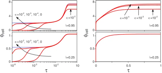
to the choice of equal values for kRand jOat both electrodes an initial DL on either electrode is absent, i.e., at = 0 the concentration, c, equals unity across the complete electrolyte phase. As a result the open cell potential equals zero. In Fig. 2 we show results for the values of the parameters discussed above and for values of⑀ranging from 0 to 10−2.
Interestingly, in case of the thin-DL limit the applied cur-rent, i, is purely Faradaic at the reaction plane during the complete transient response. For any nonzero value of⑀the applied current is initially of a purely capacitive nature in the outer共bulk兲 region, while later the capacitive nature, repre-sented by the Maxwell current, is sustained by the formation of the DLs. The Maxwell current will result in an increasing electrical field at the electrodes and thus subsequently in an increasing Faradaic current via the increasing potential drop
across the Stern layer. As a result the electrical field strength will increase until the Faradaic current reaches the value of the applied current. Consequently, for⑀⬎0 we have initially a zero cell potential which increases due to the Maxwell current, while for the thin-DL limit the cell potential is im-mediately nonzero and constant until the ions start to redis-tribute across the outer region, which is at the diffusion time scale. The initial rise time for the cell potential in case of⑀ ⬎0 is approximately=⑀as shown in Fig.2. This is in line with calculations for cells without Faradaic reactions at their electrodes, namely, for these cells it was shown that the re-laxation time scale, i.e., r=/⑀, is the characteristic time
scale关18兴. Consequently, the rise time will decrease for
de-creasing values of ⑀, such that the thin-DL limit becomes more accurate when⑀decreases. As a result, the model based on the thin-DL limit, which consists of a small set of alge-braic equations for each time, is exactly equivalent to the full PNP-gFBV theory in the limit of⑀→0.
Considering the evolution of the cell potential共Fig.2兲, we
observe that from its initial plateau, the cell potential further increases while the ions redistribute across the cell at the longer diffusion time scale. At and beyond this time scale a perfect match is observed between the thin-DL limit and full PNP model calculations when sufficiently small values of ⑀
τ
∈=10-2 , 10-3 , 10-4 , 0 ∈=10-2 , 10-3 , 10-4 , 0φ
cell 10-8 10-5 10-2 10 i=0.95 i=0.25 ∈=10-2τ
0 0.5 1 0 0.5 1 0 4 8 ∈=10-2φ
cell i=0.95 i=0.25 0 0.5 1 0 4 8 ∈=10-3 ∈=10-4FIG. 2. 共Color online兲 Cell potential as function of time for i=0.25 and 0.95,⑀=0¯10−2, k
R= jO= 10, and␦= 1共the arrows indicate
increasing values of⑀兲. ∈=10-3 , kR=jO=100
τ
φ
ce ll 10-8 10-5 10-2 10 ∈=0, kR=jO=0.1 ∈=10-3 , kR=jO=0.1 ∈=10-3 , kR=jO=0.3 ∈=0, kR=jO=0.3 ∈=0, kR=jO=100 i=0.75 0 4 8 12FIG. 3. 共Color online兲 Cell potential as function of time for
i = 0.75,⑀=0 and 10−3, k
are used. For i = 0.95, the steady-state potential decreases for increasing values of⑀. This corresponds to results presented in earlier work关31兴 where it was shown that the steady-state
cell potential at low currents coincides for all values of ⑀, while it diverges for relatively large values of ⑀ when proaching the diffusion-limiting current, i.e., for currents ap-proaching i =⫾1 关31兴. As a result, the accuracy of the
thin-DL limit does not only depend on the value of⑀but also on the value of the applied current. However, here we find that ⑀equal to 10−4 results in a near perfect match with the thin-DL limit at the diffusion time scale for currents up to
i = 0.95.
Next, we show results for three values of the kinetic con-stants, namely, kRand jOequal to 0.1, 0.3, and 100, see Fig.
3. These constants represent relatively slow共kR= jO= 0.1 and
0.3兲 and fast 共kR= jO= 100兲 reaction kinetics at the
elec-trodes. Again the results for both models, as shown in Fig.3, coincide for the times at and beyond the diffusion time scale. The results for⑀= 10−3共red lines兲 show that for low values of the kinetic constants an additional plateau value for the cell potential will appear earlier and below the plateaus as dis-cussed above. The presence of these three plateau values can be explained as follows. The applied current will first result in an increase in the potential drop across the outer region, 关60兴 as indicated in Fig. 4共a兲, leading to the first plateau value. Next, the potential drop across the outer region results in an ion flux across this region and consequently in the formation of the DLs, indicated by the increase in the poten-tial drop across the Stern layer 关Fig. 4共b兲兴, leading to the second plateau value关60兴. Finally, the potential drop across
the Stern layer results in the increase in Faradaic current at the reaction planes关Fig.4共c兲兴 and consequently in a
redistri-bution of ions across the outer region, which leads to the third and final plateau value. For high kinetic constants the first and second plateau value are indistinguishable as the potential drop across the electrochemical double layer re-mains small. For fast reaction kinetics this potential drop can remain small since only a small variation in the potential drop across the Stern layer is required for the Faradaic cur-rent to achieve the applied curcur-rent.
Furthermore, we can observe in Fig.4共c兲that the Faradaic current at x = 1 starts to increase before the Faradaic current at x = 0, with the result that when the steady-state is reached we have a slight decrease in the total number of cations in the cell, i.e., the electrolyte contains less cations than anions, a situation different from classical treatments where electro-neutrality is assumed a priori in the entire cell.
B. GC- and H-limits
The analytical expressions for the GC- and H-limits, i.e., Eqs.共26兲 and 共27兲, are based on the first-order approximation
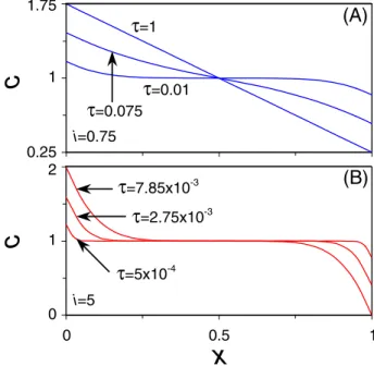
of the diffusion equation, and are thus only a good approxi-mation if the ion concentration is nearly linear across the outer region. In Fig.5共a兲we show the ion concentration dis-tribution in the outer region for different times for the thin-DL limit below the diffusion-limiting current. Figure
5共a兲shows that initially the applied current influences the ion concentration near the edges of the cell only, while the con-centration profile becomes linear when the steady-state is approached. We are already close to linear behavior at
= 0.075, which indicates that the analytical Eqs. 共26兲 and
共27兲 are a good approximation for the GC- and H-limits,
respectively. For currents above the diffusion-limiting cur-rent we do not have a linear behavior of the ion concentra-tion as indicated in Fig. 5共b兲 since we reach the transition time at ⬃7.85⫻10−3, as we will discuss in Sec. III C. In
τ
∆φ
out e r 0 1 2 (A) 0 10-8 10-5 10-2 10j
F 0.4 0.8 (C) x=0 x=1|∆φ
s|
0 1 2 (B) x=1 x=0FIG. 4. 共Color online兲 Time evolution of 共a兲 the potential drop across the outer region,共b兲 the potential drop across the Stern layer, and共c兲 the Faradaic current; i=0.75, kR= jO= 0.3, and␦= 1.
x
c
c
τ
=0.01τ
=1τ
=0.075τ
=2.75x10⁻³τ
=7.85x10⁻³τ
=5x10⁻⁴ 0 0.5 1 0 1 2 0.25 1 1.75 i=0.75 i=5(A)
(B)
FIG. 5. 共Color online兲 Concentration profiles in the outer region for the thin-DL limit for共a兲 i=0.75,=0.01, 0.075, and 1, and for 共b兲 i=5,=5⫻10−4, 2.75⫻10−3, and 7.85⫻10−3.
Fig.6 we present results for Eqs. 共26兲 and 共27兲 and for the
thin-DL limit with varying values for the Stern layer thick-ness.
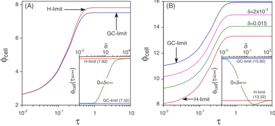
In Fig.6共a兲we present results for an electrolytic cell, i.e., the cell has a zero open cell potential and can thus not auto-generate current, which is the result of the equal kinetic pa-rameters 共kR= jO= 10兲 at both electrodes. The results show that initially the GC- and H-limits coincide, while at the steady-state there is a small difference in cell potential be-tween both these limits. The reason for the initial overlap of both curves is the relatively high value of the kinetic con-stants, which result in a relatively small potential drop across either the diffuse 共GC-limit兲 or Stern 共H-limit兲 layer. At longer times the ions will redistribute across the outer region, such that the potential drop across the Stern or DL will in-crease, which results in a difference in cell potential for both limits. This can also be seen mathematically from the discus-sion below Eqs.共26兲 and 共27兲 in the theory section. There it
was shown that the second term of Eq. 共26兲 vanishes for
large values of the kinetic constants, while the second and third term of Eq.共27兲 vanish as function of time for the same
condition. Thus, it is possible that at short times the two limits give the same results, while a difference only develops when the steady-state is reached. The inset of Fig.6共a兲shows the steady-state cell potential as function of the Stern layer thickness. It shows that for ␦= 10−2 and␦= 104the cell
po-tential for the GC- and H-limits is closely approached, while for a more realistic value of ␦ in the order of unity neither limit is exact.
In Fig.6共b兲we present results for a galvanic cell, i.e., the cell has a nonzero open cell potential and can thus autoge-nerate current. The kinetic constants for this cell are kR,A
= 300, jO,A= 1, kR,C= 10, and jO,C= 8 such that the open cell
potential equals 0= 5.48. The time-dependent behavior of
the cell potential for this case is very different compared to the previously described electrolytic cell. This is due to the fact that the applied current共i=0.95兲 is large compared to the oxidation rate constant at the anode共jO,A= 1兲, which results
in a large potential drop across the DL there. The increase in cell potential in this case follows mathematically from the
second term of Eq. 共26兲, as discussed in the theory section.
The inset of Fig.6共b兲shows that the transition from the GC-to the H-limits for increasing values of the Stern layer thick-ness differs from the behavior for the electrolytic cell plotted in the inset of Fig. 6共a兲. Here, in Fig. 6共b兲, the curve for increasing value of the Stern layer thickness shows a non-monotonic behavior, which can even break the “limiting” value of the H-limit, as already mentioned in Ref.关23兴. Still
at sufficiently small or large values of the Stern layer thick-ness the steady-state cell potential will converge to the GC- and H-limits, respectively.
C. Transition time
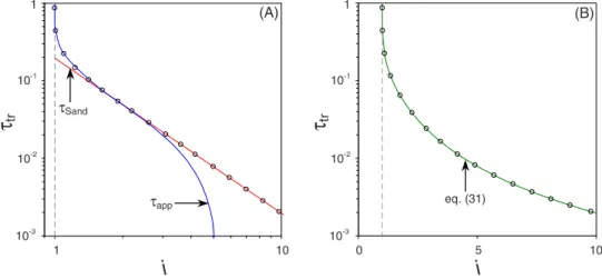
Next we show results for a cell with an applied current above the diffusion-limiting current. If we consider the thin-DL limit, the cell potential at these currents will diverge if the transition time is reached. In the previous section we showed that the implicit relation given by Eq. 共28兲 can be
used to determine the exact solution for the transition time. The explicit relation for the transition time, Eq. 共31兲, was
obtained by combining the solutions using a first-order ap-proximation for the diffusion equation, app, and the Sand
equation,Sand. The results for bothappandSand, presented
in Fig.7共a兲, coincide with the results for Eq.共28兲 in the low
and high applied current regime, respectively, while they in-tersect at i equal to ⬃2. The reason for the perfect match of
appandSandin their corresponding regime can be explained
as follows. In the low current regime the ion concentration profile across the outer region is nearly linear for longer times关Fig.5共a兲兴, a profile that is well described by the
first-order approximation of Eq. 共15兲. As a result app coincides
with the exact solution given by Eq. 共28兲 in the low current
regime. In the high current regime we can distinguish two separate diffusion layers near the electrode 关Fig.5共b兲兴, such that the similarity solution given by Eq. 共16兲 results in an
accurate description of the ion concentration. Consequently, the Sand equation, Sand, accurately describes the transition
time in the high current regime. 关Note that in Fig. 5共b兲 tr
equals ⬃7.85⫻10−3.兴 In Fig. 7共b兲 we show the results for
τ
10-1 1 10 2 4 6 8φ
ce ll 10-2 104 10 H-limit (7.82) GC-limit (7.52) 0<δ<∞ φce ll (τ =∞ )τ
10-1 1 10 8 10 12 16φ
ce ll 14 GC-limit 10-5 103 10-1 H-limit (13.32) GC-limit (15.92) 0<δ<∞ φce ll (τ =∞ ) H-limit δ=0.015 δ=2x10⁻³ (A) (B) δ δ 10-2 10-2 GC-limit H-limitFIG. 6. 共Color online兲 Cell potential as function of time for the thin-DL limit, for arbitrary␦and in the GC- and H-limits; i = 0.95;共a兲 an electrolytic cell with identical electrodes, kR= jO= 10;共b兲 a galvanic cell with different electrodes and a nonzero open circuit voltage, kR,A= 300, jO,A= 1, kR,C= 10, and jO,C= 8; insets: steady-state current as function of the Stern layer thickness.
the combined equation, Eq. 共31兲. These results show that
Eqs.共28兲 and 共31兲 coincide in the low as well as in the high
current regime. As a result we can use Eq.共31兲 as very
ac-curate analytical equation in place of the exact, implicit re-lation, Eq.共28兲.
In Fig. 8 we show results for the increase in cell potential in case of the thin-DL limit as function of time for various values of the applied current. The increase in cell potential is defined as the difference between the actual cell potential and the initial plateau value, i.e., ⌬cell=cell共兲−cell共= 0兲. Again we assume fast reaction
kinetics, i.e., kR= jO= 10, and set ␦ equal to 1. We can see
from Fig. 8 that for i = 0.5 and i = 0.9 the cell potential reaches a plateau value at the steady-state just as in Fig. 2. However, for an applied current equal to the diffusion-limiting current, i.e., i = 1, the cell potential will increase un-bounded and it will not reach a vertical asymptote as will occur for currents above the diffusion-limiting current. This behavior at the diffusion-limiting current is due to fact that at the diffusion-limiting current the concentration of reactive
ions will only reach zero concentration for tending to in-finity as explained in the theory section. At higher currents the reactive ions will reach zero concentration in finite time as indicated in Fig.8for i = 2 and i = 4 by the dashed lines.
In previous work关31,32,57兴 it was shown that the
steady-state current can break the diffusion-limiting current if a fi-nite ratio of Debye length, D, to electrode spacing, L, is
assumed, i.e., ⑀⬎0. In Fig.9 we present results for the cell potential as function of time for a system operating at i = 2 for the thin-DL limit and⑀equal 10−3and 10−2. These results show that a system with a finite value for ⑀ can break the vertical asymptote at the transition time due to the expansion of the DL at the cathode 共x=1兲 into the bulk region 关31,32,57兴.
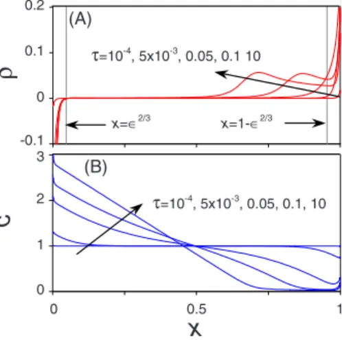
In Fig. 10共a兲 we show the space-charge density profiles across the system for various time steps. Figure10共a兲shows that below the transition time the thickness of the DL is smaller than the theoretical thickness of ⑀2/3 关31,32兴.
How-ever, for longer time the space-charge region at the cathode expands into the bulk solution, such that a charge-free outer region can no longer be assumed. The DL at the anode,
how-i
1 10 10-3 10-2 10-1 1τ
tr τSand τapp 3i
0 10 10-3 10-2 10-1 1τ
tr 5 eq. (31) (A) (B)FIG. 7.共Color online兲 Transition time as function of the applied current according to 共a兲 the two approximate solutionsSandandapp, and 共b兲 the combined solution according to Eq. 共31兲, the open circles in both panels indicate the exact solution according to Eq. 共28兲.
τ
10-3 10-2 10-1 1 i=4 0 2.5 5 10∆φ
ce ll 7.5 i=2 i=1 i=0.9 i=0.5 τtr =0 .04 9 2 τtr =0 .0 12 3FIG. 8. 共Color online兲 Increase in cell potential as function of time for currents below and above the diffusion-limiting current 共full lines兲 including the corresponding transition time 共dashed lines兲 for the thin-DL limit; i=0.5,0.9,1,2,4, kR= jO= 10, and
␦= 1.
τ
10-3 10-2 10-1 ∈=0 4 8 12 16φ
cel l τtr = 0 .0492 ∈=10-3 ∈=10-2FIG. 9. 共Color online兲 Cell potential as function of time for a current above the diffusion-limiting current for both the thin-DL limit and full model; the dashed line is the transition time; ⑀=0,10−3, 10−2, i = 2, k
ever, remains within its theoretical boundary, i.e., does not expand to macroscopic dimensions.
To summarize, we have presented results for the evolution in time of the cell potential of electrochemical cells for vari-ous parameter settings. For all the parameters that we have investigated we have obtained a good fit between the thin-DL limit and the full PNP model for sufficiently small values of⑀, except for a very brief initial period. These initial deviations can be contributed to the influence of the Maxwell current, which is included in the full PNP model but ne-glected in the simplified model. Because the Maxwell current effectively vanishes beyond a characteristic time of=⑀, the simplified model becomes more accurate at short times when
⑀decreases共i.e., for larger system dimensions relative to the Debye length兲. Furthermore, we have shown that during the start up of an electrochemical we can distinguish three pla-teau values for the cell potential, namely, a first plapla-teau value due to an increasing potential drop across the bulk region, a second plateau due to the formation of the DLs and finally a third plateau value due to the redistribution of ions across the bulk region. Next, we have shown the influence of the Stern layer thickness on the cell potential by considering the GC-and H-limits. We have shown that for an electrolytic cell with high kinetic constants the influence of the Stern layer thickness on the evolution of the cell potential is small. How-ever, for a galvanic cell with the value of one of the kinetic constant close to the applied current there is a clear distinc-tion in evoludistinc-tion of the cell potential between the GC- and H-limits, showing that in this case the influence of the Stern layer thickness is significant. Finally, we have shown that the cell potential for the thin-DL limit reaches a vertical asymptote at the transition time if the applied current is larger than the diffusion-limiting current, a limit than can be broken due to the expansion of the DL near the cathode for models where⑀⬎0.
IV. CONCLUSIONS
We have presented a mathematically simplified model for the transient 共dynamic, time dependent兲 voltage of an elec-trochemical cell in response to a current step, including dif-fuse charge effects, for a one dimensional and planar geom-etry in the limit of a negligibly thin Debye length compared to the electrode spacing. The simplified model couples a dif-fusion equation for the interior of the cell to analytic bound-ary equations that describe the diffuse layers 共space-charge region near the electrodes兲 and the Faradaic reaction kinetics. As a result, the simplified model significantly reduces the numerical complexity of the full model, which is based on the generalized Frumkin-Butler-Volmer equation for the electrochemical reaction at the electrodes and the Poisson-Nernst-Planck equation for the transport of ions throughout the electrolyte. Further, we have presented analytical equa-tions for the evolution of the cell potential in time based on a first-order approximation of the diffusion equation and the additional assumption of either a zero or infinite reaction plane to electrode spacing compared to the Debye length. The first order approximation for the diffusion equation was also used to extend Sand’s equation to the domain of large transition time 共or equivalently, currents just above the diffusion-limiting current兲.
We have shown that for applied currents below the diffusion-limiting current the simplified model is accurate at and beyond the diffusion time scale when the Debye length is small compared to the electrode spacing. For superlimiting currents the simplified model is valid up to the transition time at which the cell voltage blows up due to ion depletion in the electroneutral bulk electrolyte. In the full model we can have superlimiting currents beyond the transition time as the diffuse layer expands to a non-equilibrium structure re-sulting in charging of the bulk electrolyte. Consequently, the simplified model can be very beneficial in modeling the tran-sient response of electrochemical cells up to the steady-state for currents below the diffusion-limiting current, or up to the transition time for superlimiting currents, if the Debye length is small compared to the feature size of the cell, an assump-tion which is generally valid since the Debye length is typi-cally on the order of 1–100 nm.
In conclusion, taking into account diffuse charge effects, and thus not assuming electroneutrality in the entire cell, leads to a more insightful and comprehensive model, while the mathematical complexity of the model does not increase significantly compared to the classical models based on elec-troneutrality in the entire cell.
ACKNOWLEDGMENTS
This research was carried out under Project No. MC3.05236 in the framework of the Research Program of the Materials Innovation Institute M2i共www.m2i.nl兲. M.Z.B. also acknowledges support from U.S. National Science Foundation under Contracts No. DMS-0842504 and No. DMS-0855011.
c
ρ
x
0 0.5 1 0 1 2 τ=10-4 , 5x10⁻³ , 0.05, 0.1, 10 3 -0.1 0 0.1 0.2 τ=10-4 , 5x10⁻³ , 0.05, 0.1 10 x=∈2/3 x=1-∈2/3 (A) (B)FIG. 10. 共Color online兲 Time evolution of 共a兲 the space-charge density distribution and共b兲 the concentration profiles, vertical lines in 共a兲 indicate the theoretical inner-outer region interfaces; ⑀=10−2, i = 2, k
R= jO= 10, and␦= 1共the arrows indicate increasing