Dynamic analysis and control of a roll bending process

DYNAMIC ANALYSIS AND CONTROL OF A

ROLL BENDING PROCESS

by

MICHAEL BRUCE HALE

'B.S., Oklahoma State University

(1983)

SUBMITTED TO THE DEPARTMENT OF

MECHANICAL ENGINEERING

IN PARTIAL FULFILLMENT OF THE

REQUIREMENTS OF THE DEGREE OF

MASTER OF SCIENCE IN

MECHANICAL ENGINEERING

at the

MASSACHUSETTS INSTITUTE OF TECHNOLOGY

June 1985

(E Massachusetts Institute of Technology 1985

The author hereby grants to M.I.T. permission to reproduce and

distribute copies of

this thesis document in whole or in part.

Signature of Author

, , _-I %,v , I , v

-Department of Mechanical Engineering

June 3, 1985 Certified by

David E. Hardt

Thesis Supervisor

Accepted by

Ain A. Sonin

M~A4A

TI&partment Graduate Committee

OF TECHNOLOGY

DYNAMIC ANALYSIS AND CONTROL OF A

ROLL BENDING PROCESS

by

MICHAEL BRUCE HALE

Submitted to the Department of Mechanical Engineering

on June 3, 1985 in partial fulfillment of the requirements for the Degree of Master of Science in

Mechanical Engineering

ABSTRACT

Recent research has shown that the roll bending process can be automated by the addition of a closed-loop control

system that continuously measures the springback of the metal

workpiece. In the present work the components of a roll bending system, controlled by such a closed-loop scheme, are

analyzed to determine important dynamic characteristics of

the roll bending process. Dynamic models are developed for the individual components and for the roll bending process as

a whole.

These models are verified using an experimental

roll bending apparatus.

A linear control analysis and a

nonlinear simulation are performed, using the system model,

to determine the limits of the roll bending system response. The analysis shows that very good system response is possible

using a simple proportional controller and

proportional-plus-derivative feedback. The analysis also indicates that the derivative feedback, which for roll bending is the rate of change of unloaded curvature, can be approximated by the rate

of change of the control variable, roll velocity.

Experi-ments were performed which verified the control analysis.

The experiments also show that workpiece vibration is a major

problem as the roll bending system bandwidth is increased

because the control system is unable to distinguish between

workpiece vibration and curvature disturbances. Because the

workpiece dynamics change as the workpiece moves through the

roll bending apparatus, the control system must be designed

for the worst case. Workpiece vibration is the major factor

which limits the roll bending system response. Nevertheless,

the proposed control scheme represents a major improvement in the control of the roll bending system because of the

increased bandwidth and stability possible.

Thesis Supervisor: Dr. David E. Hardt

ACKNOWLEDGMENTS

I would like to thank Professor David Hardt for his guidance and support throughout this research. The time spent in discussion with Professor Hardt resulted in many

valuable insights.

I would also like to thank the Aluminum Company of

America for their financial support and technical

assis-tance.

Thanks also to James Owen who generously consented to examine the first draft of this document. His careful review and helpful suggestions have made the final version a much

more readable and incisive manuscript.

Finally, a special thanks to my family for their love

and support and prayers. Thanks especially to Patti whose

companionship remains a comfort and an inspiration.

TABLE OF CONTENTS

Title Page

Abstract

Acknowledgments

Table of Contents

List of Figures

Chapter 1

INTRODUCTION

Motivation

Previous Research

Thesis Overview

Chapter 2

STATIC ANALYSIS OF BENDING MECHANICS

Moment-Curvature Relationship

Straightening

Unsymmetrical Sections

Bidirectional Bending

Chapter 3

DYNAMIC ANALYSIS AND MODELING

Experimental Apparatus

Workpiece Model

Servo Model

Measurement and Filter Model

Disturbance Model

Controller Model

Chapter 4

CONTROL

Control Objectives

Linear Control Analysis

Page No. 1 2 3 4 6 10 10 11 15 17 17 23 26 32 34 35 38 45 49 49 53 55 56 60 I

Chapter 5

Nonlinear Control Analysis

EXPERIMENTATION

Experimental Objectives

Experiments

Step Tests

Disturbance Tests

Chapter 6

CONCLUSIONS

Future Research

Bibliography

Appendix 1 EXPERIMENTAL BENDING APPARATUS

Appendix 2 MEASUREMENT ALTERNATIVES

Loaded Curvature Measurement

Moment Measurement

Bending Stiffness Measurement

Appendix 3 ERROR ANALYSIS

Appendix 4 COMPUTER PROGRAMS

Bending Control Program

Modeling Program

Step and Frequency Response Program

73 79 79 83 84 109 115 118 122 125 141 142 149 152 155 159 159 169 174

LIST OF FIGURES

No.

Pyramid 3-Roll Bender Configuration

Stress State in a Loaded Beam

Moment-Curvature Relationship

Momient vs. Workpiece Position

Roll Bender Configuration

Closed-Loop Control Block Diagram

Shifted Moment-Curvature Diagram

Triangular Rod

K vs. Center Roll Position

u

Experimental Roll Bending Apparatus

Roll Bending System Block Diagram

Elastic-Perfectly-Plastic Stress-Strain

1/8" X 1" Aluminum Workpiece Model

1/4" X 1" Aluminum Workpiece Model

Workpiece Hysteresis

Hysteresis Test

Velocity Servo Step Response

Velocity Servo Bode Diagram

Position Servo Step Response

Position Servo Bode Diagram

Filter Bode Diagram

Disturbance Model Block Diagram

Disturbance Detection

Page No. 12 18 18 20 20 24 24 27 33 36 36 38 41 41 43 43 47 47 48 48 50 51 51

Figure

1 2 3 4 5 6 7 8 9 10 21 12 13 14 15 16 17 18 19 20 21 22 23

24

Discretized Control Output

54

25 Disturbance Block Diagram 62

26 Position-Servo Based Block Diagram 65 27 Velocity-Servo Based Block Diagram 65

28 Position-Servo Based Root Locus 66

29 Velocity-Servo Based Root Locus 66

30 Velocity-Servo Based Z-Plane Root Locus 69

31 Z-Plane Root Locus with a Zero 69

32 Simulated System Step Response 77

33 Simulated System Step Response 78

34

Simulated System Disturbance Response

78

35 Test #1 Plot #1 85 36 Test #1 Plot #2 85 37 Test #1 Plot #3 86 38 Test #1 Plot #4 86 39 Test #2 90 40 Test #3 92 41 Test #4 92 42 Test #5 96 43 Test #6 96 44 Test #7 98 45 Test #8 98 46 Test #9 Plot #1 99 47 Test #9 Plot #2 99 48 Test #10 100 49 Test #11 103

50 Test #12 Plot #1 103 51 Test #12 Plot #2 104 52 Test #13 107 53 Test #14 107 54 Test #15 Plot #1 108 55 Test #15 Plot #2 108 56 Test #16 Plot #1 112 57 Test #16 Plot #2 112 58 Test #17 Plot #1 113 59 Test #17 Plot #2 113 60 Test #18 Plot #1 114 61 Test #18 Plot #2 114

62

Roll Bender Hardware Relationships

127

63

Outer Roll-Pair Rotation

128

64 Center-Roll Housing 129

65

LVDT Curvature Measurement Device

131

66 LVDT Noise 132

67 Potentiometer Noise 132

68 Force Transducer and Potentiometer 134

69 F Noise 135

x

70 F Noise 135

y

71 Roll Bender Geometry 136

72

Curvature Measurement Scheme

137

73

Translated Moment-Curvature Origin

143

74 LVDT Configurations 143

76 Measurement Errors 157

Chapter 1

INTRODUCTION

Motivation

In an effort to increase productivity and remain competitive in the world market, many companies are

consid-ering production process automation.

In the metal forming

industry much interest has been generated by the introduction

of automation for traditionally manual operations such as

brakeforming and roll bending.

The first generation of

automation for these processes was the addition of a simple position servomechanism and controller. On a brakepress, for

example, a position servomechanism (servo) enabled the

operator to program a series of movements which could be

repeated very quickly and precisely.

This did not

signi-ficantly improve productivity, however, because of the

extensive reworking needed to achieve the necessary shape

accuracy.

Even though the brakepress position could be

controlled very closely, final part shape varied because of material property variations. More recent work by Hardt [1], Allison and Gossard [2], and Stelson [3] has shown that a

material adaptive control scheme can be developed for the

brakeforming

process

which

will

significantly

improve

productivity by explicitly accounting for material properties

in-process.

bending process, is used in many metal forming situations

that fit within the particular hardware restraints. The roll bending process, where applicable, is much faster than the

brakeforming process because rather than forming the material

in discrete steps, as in brakeforming, the workpiece is

formed continuously as the material is rolled through the

machine.

The advantages of the continuous forming provide

the motivation for the research presented in this thesis. The roll bending operation has great potential as an effi-cient and versatile metal forming process. The goal of this research was to develop an automatic control scheme for the roll bending process that would take advantage of the inher-ent speed of the roll bender while incorporating a

closed-loop control scheme.

Previous Research

The three-roll pyramid roll bender shown in Figure 1 is a typical configuration that consists of a pair of fixed outer rolls and a movable center roll. One or more of the rolls is driven, and friction between the rolls and the work-piece permits the material to be rolled through the machine. As the workpiece moves, the center roll is adjusted to pro-duce a variable bend along the length of the workpiece. This process is used to form long flat workpieces such as heavy plate used in boilers and reactor vessels. Roll bending is also used extensively to form long thin workpieces such as

Final

Shape Workpiece Movable

Center

Roller

4

Fixed

Outfeed

Roller

Fixed

Rollnfeed

Roller

Figure 1. Pyramid 3-Roll Bender Configuration

aluminum extrusions. In the aluminum industry roll bending

is also used for final straightening and contour correction of extrusions. This operation is entirely manual and the accuracy of the final product shape is dependent on the skill of the operator.

In recent years some effort has been directed toward

automating the roll bending process.

The major obstacle

confronting researchers has been material springback.

In

roll bending, the metal workpiece is plastically deformed as

the workpiece moves through the machine.

As the workpiece

exits the bending apparatus the elastic stresses in the metal

are relaxed and the metal "springs back". Thus the metal

does not obtain its final shape until the workpiece has exited the machine. Some of the earliest attempts to deal with the material springback problem (Sachs [4] and Shanley [5]) used empirical data to characterize springback for

certain materials and workpiece shapes. Other researchers

([6] to [14]) used various analytical methods in an attempt

to predict stress and strain conditions as well as springback

for various materials.

Later, Hansen and Jannerup [15]

developed a more complex model for elastic-plastic bending of

beams that could be used to obtain a more nearly accurate

estimate of the workpiece springback.

Cook, Hansen, and

Trostmann, [16] 'ised the beam model in [15] to design an

open-loop controller for a roll bending machine and

demon-strated that good control of the final part shape is possible

if the material properties, including springback, are known

beforehand.

The condition of prior knowledge of material

properties is very restrictive, though, and seriously limits

the usefulness of the controller. Foster [17] developed a machine which measures the final part shape as the workpiece

exits the bending apparatus.

This measurement can be

incorporated into a closed-loop curvature controller.

The

advantage of this type of control scheme is that no prior

knowledge of material properties is required for controller

implementation. The curvature measurement, though, is taken

after the workpiece has exited from the bending apparatus.

At this point the workpiece already has been formed to its

final shape so the information cannot be used to correct the current error, but only to maintain a relatively constant

final curvature. More recent research by Hardt, Roberts, and

Stelson [18], in the area of roll bending, and similar research by Gossard and Stelson [19], in the area of brake-forming, has shown that it is possible to measure the

important material properties, including springback, during

forming and thus design a closed-loop controller for these processes. Hale and Hardt [20], and Lee and Stelson [21] have extended the approach in [18] to include the roll

straightening process and have conducted experiments that

show that with a closed-loop controller, straightening is

nothing more than bending to zero curvature.

Although the

control scheme presented in [18] works well in theory, the

productivity gains possible with this closed-loop curvature

controller are limited by the assumption that workpiece

feedrate will be very slow. This assumption was necessary to

avoid unwanted oscillation and instability. In [18] and [20] the feedrates are kept below 0.7 in/sec. In [21] the

work-piece was actually stepped through the bending device and the

forming was performed while the workpiece was stationary.

This closed-loop control method enhances the versatility of

the roll bending process by making one-pass forming of

arbi-trary shapes possible, but it does not exploit the inherent speed advantages of the roll bending process. Thus much of the possible productivity gains are lost.

Thesis Overview

The work described in this thesis presents a new control

method

that greatly improves the

roll bending system

response. In Chapter 2, a complete static analysis of the roll bending process is presented. In addition, three

bending cases that merit special attention: straightening,

forming unsymmetrical sections, and bidirectional bending,

are examined in some detail to determine how the control approach presented in [18] must be modified to apply to these cases. In Chapter 3 the roll bending system is broken down into five primary components. Models of each of these five

components are developed to determine their individual

influence on system dynamics and response. These models are

verified using an experimental bending apparatus that is

described briefly in Chapter 3 and in more detail in Appendix 1 and [22]. In Chapter 4 the dynamic models are used to

develop a digital controller that satisfies specific control

objectives.

The relative importance of the control

objec-tives listed in Chapter 4 varies according to the type of bending, so the control analysis is presented first in gene-ral terms and then examined using the experimental apparatus

for specific types of bending. This analysis indicates that

the roll bending system bandwidth can be greatly increased by

a simple modification to the control system presented in

[18]. Using a proportional-plus-integral controller with a

velocity servo results in a much simplified dynamic system

with good stability and improved bandwidth. The new control

method presented allows the same system response to be

maintained at much greater feedrates, resulting in large

productivity gains for very little cost. The experimental procedures and results are presented in Chapter 5. The results verify the models developed in Chapter 3 as well as the new control method proposed in Chapter 4. Chapter 6

contains the conclusions and also some suggestions for future

research. The major conclusion is that there is a rather

severe limitation imposed on maximum system bandwidth because

of workpiece vibration. More research is needed to

charac-terize completely the effect of the workpiece vibration on

the final curvature of the workpiece. In addition, a more detailed study of the mechanics of bending could yield some insight into the problems and possibilities of one-pass

two-dimensional and three-dimensional bending.

The

appen-dices contain more detailed information on the experimental

hardware and software as well as an error analysis and

hard-ware concerns and measurement alternatives.

Chapter 2

STATIC ANALYSIS OF BENDING MECHANICS

The closed-loop curvature control scheme for both the roll bending process and the brakeforming process is based on

real-time measurement of the material springback. The

devel-opment of this control scheme is repeated below.

Moment-Curvature Relationship

A work?iece in a three-roll bending machine can be modeled as a beam under three-point loading as shown in Figure 2. As the beam is loaded, the material is initially stressed elastically. If the beam is loaded so that the stress in the beam is always below the yield stress, then when the beam is unloaded, the material will "spring back" and regain its original shape. If, however, the beam is loaded so that some of the fibers are loaded past the elastic limit, then the beam is plastically deformed and will be

permanently deformed when unloaded.

Figure 2 shows the

stress state in a beam that is loaded past the yield point. The final workpiece shape depends on the initial shape, the initial stress state, and the stress distribution, all as a

function of position along the workpiece. The relationship

between the stress state of a workpiece and the resulting curvature can be seen in the moment-curvature relationship, which can be derived from the stress-strain relationship.

zone

Figure 2. Stress State in a Loaded Beam

C B dM dK D KL

Curvature

Figure 3. Moment-Curvature Relationship

M

c

E 0 A _ · _

Figure 3 is a general moment-curvature diagram for an ini-tially flat workpiece. This diagram is drawn for a single point along the length of the workpiece. A similar diagram is needed for every point on the workpiece to characterize completely the workpiece curvature. The situation can be greatly simplified by considering the geometry of the

three-roll bending process.

For a workpiece that is loaded in a roll bending

appara-tus, the exact moment distribution along the sheet is complex

but can be approximated as a linear function of arc length assuming that no moment is generated between the drive rolls and the workpiece (Figure 4). As indicated for three-point

bending, the bending moment applied to the workpiece

increas-es from zero at the input roll to a maximum at the center-roll contact point and then decreases to zero at the output roll. This loading sequence can be traced on the

moment-curvature diagram (Figure 3), the moment-position diagram

(Figure 4), and on a machine diagram (Figure 5). At the input roll the workpiece has zero moment and, assuming an initially flat workpiece, zero curvature (Point A). The moment and

curvature increase and the workpiece deforms elastically

until the yield point is reached (Point B). The slope of the

elastic loading line in Figure 3 is the effective bending

stiffness. As the moment increases from Point B to a maximum at Point C the sheet deforms plastically. The moment and

curvature decrease linearly as the sheet moves from maximum

d2

C

B

Position

Figure 4. Moment vs. Workpiece Position

Workpiece

Movemenf

_inch

Roller

Figure 5. Roll Bender Configuration

,,4-c

E

o

loading (Point C) to the output roll (Point D) where the moment is again zero but the curvature is not because the workpiece has been plastically deformed. The slope of the unloading line in Figure 3 is the same as the elastic loading line. The workpiece springback as a function of distance, s,

along the workpiece is the difference between the maximum

loaded curvature and the final unloaded curvature and is found from Figure 3 to be:

AK(s) = KL(s) - K (s) (1)

U

where KL is the maximum loaded curvature and K is the

L ~~~~~~~~u

unloaded curvature. The springback can also be expressed in terms of the moment. As shown in Figure 3 the unloading path is a linear function of the moment and so the springback can be expressed:

AK(s) = M(s)/(dM/dK) (2)

where M(s) is the moment distribution along the sheet and dM/dK is the slope of the elastic loading line. This equation points out one of the major advantages that the roll

bending process has over the brakeforming process.

For

brakeforming, where the workpiece is formed at discrete

loca-tions, it is necessary to obtain the full moment-curvature distribution along the workpiece in the forming region to

predict accurately the distributed springback.

For roll

forming, however, every point along the workpiece is loaded to the maximum moment as it passes under the center roll, and

by controlling the maximum moment, each point along the

workpiece can be formed individually.

As shown in [22], if the loaded curvature and the springback are known for a given point, then the unloaded curvature is found by rearranging Equation 1:

K = KL - AK (3)

u L O

This can be combined with Equation 2 to yield:

K

_u

= KL -

Mmax/(dM/dK)

(4)

where it is understood that these two equations apply to each point along the workpiece. Equation 4 shows that it is possible to calculate the unloaded curvature of the work-piece while the workwork-piece is in the loaded condition if the

moment and curvature at the contact point under the center

roller are known together with the bending stiffness of the

workpiece. In other words it is possible to measure the

material springback in real time. Because the measurement is made at the center roll where the forming occurs, there is no measurement lag as there is with post-forming measurements as presented in [17]. A closed-loop controller can be designed using the unloaded curvature as the loop feedback. A general block diagram of such a control scheme is presented in Figure 6. A control system based on the real-time measurement of springback has many advantages over systems based on delayed measurement or springback prediction, such as in [16]. The

primary advantage is that one-pass forming of arbitrary

shapes is possible because the controller can use the actual

system output, unloaded curvature, for feedback. Thus the

system shown in Figure 6 can be thought of as a closed-loop curvature servo. Changes in material properties such as yield point, which can differ from workpiece to workpiece and even along the same workpiece, are reflected in the moment

and curvature measurements and compensated for

automati-cally. This was demonstrated for the static case by Hardt, Roberts, and Stelson in [18] and Roberts in [22].

Straightening

Another significant advantage of real-time measurement

of unloaded curvature is evident in the straightening

application. Consider a workpiece that is initially curved.

The effect of the initial curvature on the moment-curvature diagram is shown in Figure 7, which is drawn for a single

Desired Error Rolls Workpiece

4 F t Controller iS ervo Roll Work piece

I I I I I

Ku Measured

KL Measured I

Moment Measured

Figure 6. Closed-Loop Control Block Diagram

Yield Point

r i U. y U Curvuture

Figure 7. Shifted Moment-Curvature Diagram

..-E 0

Initial

Curvature

I I I I I I

I

- . -±& ,& K I I d M/d K

point on the workpiece where the initial curvature is nega-tive. The initial curvature simply shifts the origin of the

curve. In the unloaded state (zero applied bending moment)

the loaded curvature is no longer zero and the curve shifts to reflect this initial condition. The actual shape of the

nonlinear portion of the curve depends on the initial stress

state in the workpiece. The slope of the loading and unload-ing lines does not change though, so the control scheme is

unaffected by initial stresses. In the closed-loop

control-ler, initial curvature can be described as a system distur-bance. A model of this disturbance is developed more fully in Chapter 3. The closed-loop control scheme will sense the

disturbance and react to eliminate it. Because the

distur-bance is measured under the center roll, the control system

can react while the workpiece is still loaded. Thus, with

the closed-loop controller, straightening is no different

than bending to zero curvature and can be accomplished in a

one-pass operation without prior knowledge of the

distur-bance. This is clearly not possible using predictive methods

of calculating the springback unless the disturbances are

fully known beforehand. Prior knowledge of the disturbances

requires a separate operation and additional instrumentation,

and even then, multiple passes may be required because a

controller based on predicted springback is open-loop and

cannot compensate for material property variations.

Unsymmetrical Sections

For a workpiece with a cross-sectional area that is symmetric about a given axis and material properties that are constant along the workpiece and symmetric about the axis, a pure moment acting in the plane of symmetry will produce a

deflection only,

in the plane of symmetry, These conditions

are very restrictive though, and apply only to a limited number of industrially relevant cases. The general case of

three-dimensional bending is much more complex.

For an

arbitrary cross-section with a bending moment applied in an

arbitrary direction, it is possible for the workpiece to

twist about the longitudinal axis and bend about two

orthog-onal transverse axes. In other words, the two-dimensional bending and the twisting are all coupled and may all occur

from a one-dimensional loading.

Consider a triangular rod (Figure 8) that is loaded about the two orthogonal transverse axes. The deflection in the xy plane is related to the loading by Equation 5 (see [23] and [24]):

a

MzI

+M T

YZ

(5)

as E(I I - I 2

yy zz yz

where _{is the local beam angle in the xy plane, s is the} distance along the beam, E is the modulus of elasticity, M

_M

Figure 8. Triangular Rod

and M are the moments applied about the z and y axes y

respectively, I and I are the area moments of inertia for

zz yy

the z and y axes respectively, and I is the area product of

yz

inertia for the y and z axes. The deflection in the xz plane

is:

a

-MzIY As E(I I

yy zz

- M I YY - I 2)

yz

where is the local beam angle in the xz plane. It is easy to see that a moment applied only in the z (or y) direction

(6)

will produce a deflection in two directions because of the coupling from the product of inertia term, Iy_{z .} This

multi-y z

dimensional bending is undesirable for the roll bending

process because three dimensions must be measured and

controlled in order to control the final shape for the general case. Therefore it is important to analyze the coupling effect to determine how it can be prevented or reduced.

From Equations 5 and 6 it is obvious that the bending is uncoupled when I = 0.0. This is the case if y and z are

yz

principal axes, such as the axes through the centroid and

parallel to the edges of a rectangular section. Thus bending

about a principal axis will result in an uncoupled deforma-tion. For many sections however, this restrictive condition cannot be met. Even if coupling is unavoidable, the effects

can be minimized.

Because permanent changes in curvature

involve plastic deformation, if a moment in one direction

produces plastic deformation in one direction and elastic

deformation in all other directions, the bending is

effec-tively uncoupled. Although bending occurs in more than one

direction, plastic deformation, and therefore permanent

curvature changes, will occur in one direction only. The

following analysis demonstrates the effect of coupling for a

two-dimensional case.

Suppose that the workpiece shown in Figure 8 is ini-tially flat and is loaded in a single direction (M = 0.0).

Rewriting Equation 6 gives:

-M I

as E(II - I

2)(7

Rewriting Equation 5 yields:

Da MzIzz

= "

2

(8)

as E(I _{yy zz} Izz - IZ _yz )

Substituting Equation 8 into Equation 7 yields:

(as

)(acz)

'1(9)

as \

as

From this equation it is easy to see that the coupling is governed by the ratio of the product of inertia to the moment of inertia. A similar development cn be used to show that the coupling that occurs when M = 0.0 is given by:

z

as

Iz

I

(10)

as

I

yy

Now let K be the maximum elastic loaded curvature in the xz xz

plane and K be the maximum elastic loaded curvature in the

xy

xy plane. Then the conditions that will ensure uncoupled bending are given by:

QCz)()

Kxz(l

as

(11)

z/

for bending in the xy plane and

(I)(

as)

2xy

Y Y

for bending in the xz plane. Consider, for example, the triangular cross section shown in Figure 8 where h = 1.75 in, b = 1.25 in, E = 10x106 psi and the proportional limit is

35x103 psi (Aluminum 6061-T6). If the maximum elastic loaded

curvature can be approximated by the loaded curvature of the

workpiece when the outermost fibers are stressed to the

proportional limit, then:

.4

I = 0.186 in zz

.4

I = 0.095 in Yy

.4

I = -0.066 in yz K = 0.004 in xz K = U.u03 in xy

Thus the largest curvatures that can be formed in each

direction without affecting the unloaded curvature in the

other direction are:

S -- (0.004) = 0.011 in (13)

as

\

yz

-

--

(0.003)

0.0043 in

1

(14)

as

For straightening the triangular beam, it might be possible to keep the curvature below the indicated values because curvature magnitudes are very small. For bending, though, coupling is sure to occur. But the coupling effect can be

minimized by careful application of the analysis shown

above. By bending first in the direction which is least

affected by bending in the opposite direction, the required

number of passes will be minimized if an iterative control method is used. Better yet, it might be possible to calculate, using Equations 9 and 10, the overbend or

underbend needed to compensate for the coupling.

This

defeats the purpose of the closed-loop control scheme

however, because the coupling is estimated and not measured

explicitly.

If the closed-loop curvature control scheme

could be applied to two or three dimensions then the coupling effects would be measured and compensated for automatically,

much like initial curvature disturbances are handled in

straightening. The work presented here will be restricted to

one-dimensional uncoupled bending to simplify the

eperi-mental apparatus.

Bidirectional Bending

To form arbitrary workpiece shapes in a single pass the

bending apparatus must be capable of forming both positive

and negative (bidirectional) curvatures.

This means that

more complex hardware, such as opposing roll pairs, is needed

(see Appendix 1). The closed-loop control scheme can be

applied to bidirectional bending with no changes. The major

difference between unidirectional and bidirectional bending

is due to the effect of the elastic deadband region. Equa-tion 4 together with Figure 3 show that there is no change in

the unloaded curvature while the workpiece is loaded

elasti-cally. Thus for a certain range of center-roll movement the system output does not change. This range of movement is

called the deadband region. Figure 9 shows the relationship

between center-roll displacement and unloaded curvature for a

workpiece that is stationary in the bending apparatus. The

points noted in Figure 9 correspond to the loading conditions

shown in Figure 3 for the special case of a stationary work-piece. Notice that a large portion of the loading path and the complete unloading path shown in Figure 3 are in the

deadband region. For unidirectional bending with no

over-shoot, the system passes through the deadband region only

once at the start of bending and the effect on the system response is very small. For bidirectional bending, and

especially for straightening where curvature levels are very

small, most of the center-roll movement may be in the dead-band region. Thus it is possible for the deadband region to

dominate the system response. This is of little importance

for static bending but becomes very important for the dynamic

case where the workpiece moves through the roll bending

appa-ratus. The deadband region has a large effect on system

stability and error, especially as the feedrate becomes

large. The effect of the deadband region on the system

dynamics will be explored in more detail in the next

chapter.

Ku _-mm~ D

/

=

/~~~~~~~~~~~~

/F

/ Deadband -o T I C~~~~

B

Center Roll

-. NPosition

'Deadband

P

Figure 9. K vs. Center-Roll Position U

Chapter 3

DYNAMIC ANALYSIS AND MODELING

The research presented in [18], [20], [21], and [22]

demonstrated that the closed-loop control scheme described in

Chapter 2 works very well for bending and straightening if the workpiece is rolled through the apparatus very slowly. The assumption of very low feedrate allowed the authors to ignore any dynamics associated with the servo system or workpiece. In this chapter a model of the roll bending

system that includes dynamic effects will be developed. This

model will be used to analyze the dynamic performance of the roll bending operation and predict the performance limits. Then the dynamic model will be used to develop a control algorithm. The system dynamics for any roll bending appara-tus will depend on the particular roll bending configuration and hardware under consideration. A general roll bending

system must contain several key components to implement the

closed-loop controller. The dynamic models of these

compo-nents are presented in general terms later in this chapter. These models are used to analyze a particular roll bending configuration that was used to perform the experiments in Chapter 5. The experimental roll bending apparatus is used to examine the validity of the dynamic models and also to

develop and evaluate different controllers. A short

descrip-tion of the experimental apparatus is given below. More

detailed information about the experimental hardware is

presented in Appendix 1 and [22].

Experimental Apparatus

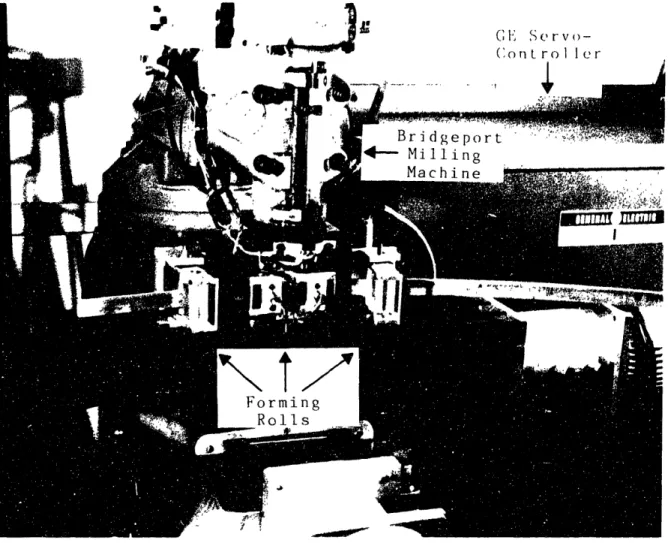
The experimental bending apparatus (Figure 10) consists

of two outer roll-pairs and a center roll-pair mounted on a Bridgeport milling machine. All of the roll-pairs have a fixed roll and an adjustable opposing roll. Thus the appa-ratus is capable of bidirectional bending of various sized

workpieces. The outer roll-pairs are fixed to the milling

machine bed which is driven by DC motors through a

ball-screw. The movement of the outer rolls with respect to the

center roll provides the forming action needed. The center

roll is mounted in and driven by the milling spindle. The workpiece is clamped between the driven center roll and the opposing center roll. Friction between the rolls and the

workpiece causes the workpiece to move through the

appara-tus. Feedrate can be varied by adjusting the spindle speed. As shown in Equation 4, the loaded curvature and the maximum

moment must be measured to implement the closed-loop control

scheme.

Loaded curvature is measured on the experimental

apparatus by two linear variable differential transformers

(LVDT's) which are mounted next to the center roll. The

distance between the LVDT's is adjustable.

The maximum

moment is measured with a strain-gage force transducer.

Figure 10. Experimental Roll Bending Apparatus

Ku

Figure 11. Roll Bending System Block Diagram

+

Notice that all the roll-pair housings are free to rotate so that no moment is generated between the rolls and the work-piece. The rotation of the roll housings changes the moment arm used to calculate the maximum moment and therefore the

rotation must be measured.

Rotation of the center-roll

housing is measured with a potentiometer. The outer-roll

rotations are negligible for the bending experiments reported

in Chapter 5 and are not measured. Appendix 3 contains a complete error analysis which shows the effect of neglecting

various measurements. Appendix 2 presents some alternatives

to the moment and curvature measurements.

Analog signals

from all transducers are amplified and filtered before being sent to a computer where they are digitized. The computer then uses this information to generate an error signal which is sent to a General Electric servo-controller. The servo-controller is connected to the DC motor that adjusts the roll position and the loop is completed.

Analysis of the machine description and the bending

process reveals five system components that appear to

contribute significantly to the system dynamics. These five

components are the workpiece, the servo system, measurements and filters, disturbances, and the system controller. A

block diagram of the roll bending system which includes all

these components is shown in Figure 11. A model for each of

these components is developed below and verified using the

experimental apparatus described.

Workpiece Model

As shown in Chapter 2 it is not necessary to know

anything about the plastic deformation of the workpiece as it is being loaded to measure the unloaded curvature. It is only necessary to know the maximum moment and curvature at each point along the workpiece and the slope of the unloading path. For modeling purposes however, it is necessary to know how the workpiece deforms, both elastically and plastically as a function of the center-roll position. For the workpiece model we will assume that the workpiece material is

elastic-perfectly-plastic, which means that the stress-strain

rela-tionship is as shown in Figure 12. In the elastic region the

0

I.

-C')

Strain

moment and curvature are linearly related by the bending

stiffness. If we further assume that the workpiece has a

rectangular cross section that is constant along the length,

then the relationship between moment and curvature for the entire loading path can be described as shown in [23] by:

M = K(dM/dK) K < K

Y

(15) M = 1.5M (1 - (K /K)2/3) K K

y y y

where M and K are the moment and curvature at yield.

Y Y

The curvature of the workpiece can also be expressed as

a linear function of roll position using the deflection

equation of a beam under three-point loading,

K = 3z/(L ) (16)

where z is center-roll displacement and L is the distance

between the center and outer roll.

This relationship is

based on linear beam theory, but is a very good approxima-tion well beyond yield as shown in Figures 13 and 14. This equation is not dependent on material properties such as bending stiffness or yield point and is therefore very useful for a general model.

following relationship between unloaded curvature and

center-roll displacement (assuming an initially flat workpiece):

K = 0.0 z < z u =°° y (17) 3z 9zz 3 K - - Y + a u L2 2 L2z2 y

where zy is the center-roll position at the yield point of

the workpiece.

Equation 17 is the desired workpiece model

that relates the input (center-roll position) to the output

(unloaded curvature). This equation applies to the point on

the workpiece that is in contact with the center roller (Point C in Figure 5). As shown in Chapter 2, this point

corresponds to the maximum moment and curvature which means

that the final curvature of the workpiece is set at this point. Applying Equation 17 to each point on the workpiece as it is rolled through the apparatus provides a model of the workpiece as a function of the distance along the workpiece.

Figures 13 and 14 are plots of measured moment scaled by

the bending stiffness, loaded curvature, and unloaded

curva-ture versus roll position for a 1/8" X 1" 2024 aluminum strip and a 1/4" X 1" 2024 aluminum strip, respectively. Equations 15, 16, and 17 are also plotted using the bending stiffness

and yield point obtained by experimentation.

These plots

0 2 4 6 8 10 12 14 16 1 E CENTER ROLL POITION INDO

Figure 13. 1/8" X 1" Aluminum Workpiece Model

E-03 o"n ____ ____ __ __ _ Ou 70 60 x 50 U z - 40 w 30 20 10 to0 _inl 20 E-01 0 1 2 3 4 5 6 7 8 9 10 E-o01

CENTER ROLL POSITION (INCH)

Figure 14. 1/4" X 1" Aluminum Workpiece Model

E-02 I0 14 12 :r 10 :z to U

z

N 8 w cr, M 6 I-n3 4 U 2 0 -2 IU I

show that the workpiece model developed above is a reasonable

approximation of the actual workpiece.

There are three important features to note from the workpiece model. First, there is a deadband region while the workpiece is elastically loaded. The significance of the deadband region depends on the type of bending and the bend-ing stiffness of the workpiece. For very stiff workpieces the elastic region, and therefore the deadband region, is very small. Flexible workpieces have a much larger deadband

region. Forming circular shapes or bending workpieces with

curvatures in only one direction involves passing through the

deadband region only once. For bidirectional bending or for

straightening, the deadband region may dominate the operating

region for a particular workpiece.

The second important feature of the workpiece response

is that the response has two different forms depending on

whether the workpiece is stationary or moving through the

rolls. For a stationary or very slow moving workpiece, there is hysteresis in the model as shown in Figure 15. This is

because the unloaded curvature does not change while the

workpiece is in the elastic loading state or during unload-ing. If the workpiece is stationary, then the same portion of the workpiece is formed during a forming cycle. For a

moving workpiece, each point along the workpiece is formed

only once since new material is continually fed into the

bending apparatus. Figure 15 shows that a moving workpiece

Stationary Workpiece Moving Workpiece Ku Position

Figure 15. Workpiece Hysteresis

E-02

cl

0 1 2 3 4 5

TIME (SEC)

Figure 16. Hysteresis Test

7 8 x -.J 1y m xy 5 4 3 2 1 0 -1 -2 E*00 a

does not have hysteresis but still has a deadband region.

Figure 16 shows the dramatic effects of the workpiece

hyster-esis. This figure shows the loaded and unloaded curvatures

and the scaled moment for a stationary 1/4" X 1" aluminum workpiece such as the ne described in Figure 14 in response

-1

to a step curvature command of 0.01 in . The deadband region is apparent in the first 0.25 sec, but then the

unloaded curvature responds quickly to move to the commanded

value. The system has a very small overshoot and the roll position decreases in an attempt to eliminate the error. But

even though the moment and loaded curvature decrease, the

workpiece is unloading elastically as indicated in Figure 3

and the unloaded curvature does not decrease. When the workpiece is loaded past the negative elastic limit the

unloaded curvature will decrease and the error will be

eliminated. This occurs at about 3.75 sec in Figure 16. This response is exactly the response indicated by the hysteresis shown in Figure 15. The results n Figure 16 can be compared to the results of Test 10 shown in Chapter 5, which is the same test with a moving workpiece.

The third important feature to note about the workpiece model is that time is not a variable in the model. The

unloaded curvature is a function of center-roll position

only. This means that the workpiece can be thought of as a

nonlinear gain. This is, of course, an approximation because

the workpiece does actually have mass, compliance, and

damp-ing, which will all affect the system dynamics. In the

workpiece model these effects are assumed to be negligible.

This assumption turns out to be a critical feature of the model, which is valid only under certain conditions as shown

in Chapter 5.

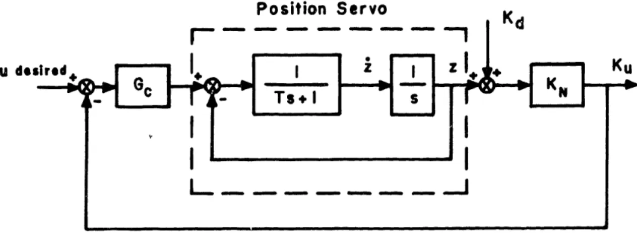
Servo Model

The roll bending apparatus works by adjusting the

center-roll position to change the loading in the

work-piece. Closed-loop control of the roll bender requires

auto-matic control of the center-roll position by a servo system.

There are several different roll positioning alternatives

available on commercial roll bending machines. Actuation can

be achieved using a hydraulic servo system or a DC motor and

leadscrew, for example. At low frequencies the servo systems

can all be modeled as a standard position servo or velocity servo. The equation for a position servo, expressed in

Laplace transform notation, is:

2 z w n = 2 (18)

z

s + 2w

+ w

C n n

where z is the position command, wn is the natural frequency, and is the damping ratio. The equation for a

velocity servo is:

-z K

T (19)

zc Ts + 1

C

where z is the center-roll velocity, zc is the velocity command, K is the servo gain constant, and T is the system time constant.

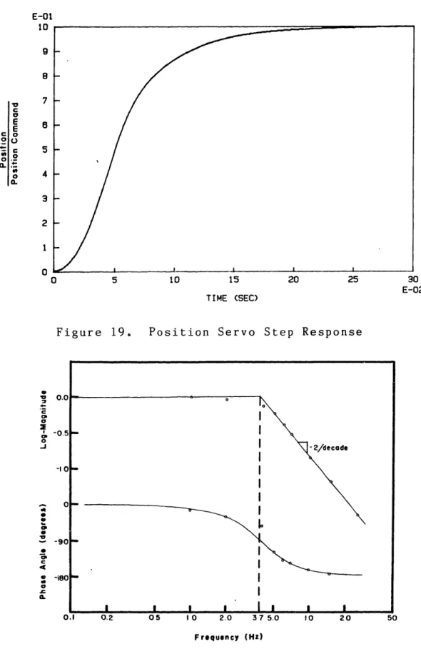
The GE servo-control system on the experimental bending apparatus can be configured as either a velocity servo or a position servo. Figure 17 is a plot of the center-roll velocity in response to a step input to the velocity servo. Figure 18 is a Bode diagram which shows the frequency response of the velocity servo. The forcing function used to drivre the servo and determine frequency response was gener-ated from the control computer. This was done to ensure that all the electronics are included in the dynamic response. The program used to determine the step and frequency response is listed in Appendix 4. Figures 17 and 18 indicate that the

velocity servo is a first-order system with a time constant

of 0.042 sec. Thus the servo model given by Equation 19 is a very good approximation to the actual system if T = 0.042. The servo gain constant, K, is adjustable on the GE servo-control system. For modeling purposes the servo gain con-stant is assumed to be 1.0 so that all of the system gains are represented by the controller gain. Figures 19 and 20

5 10 12.6 15 20 25

TIME (SEC)

Figure 17. Velocity Servo Step Response

Frequency (Hz)

Figure 18. Velocity Servo Bode Diagram

E-O1 o10 9.5 9 a C E E 0

0

>

3. U 0 0 t 7 6 5 4 U oa 3 2 I 0 0 30 E-02 a 0

-i

. .

5 10 15 20 25

TIME (SEC)

Figure 19. Position Servo Step Response

0.2 05 10 2.0 37 5.0 10 20

30

E-02

50 Frequency (Hz)

Figure 20.

Position Servo Bode Diagram

E-01 'U 9 8 7 C E E .oo 03. 0 a. 6 5 4 3 2 I 0 0 C 41 J . 0. -0.5 -I 0 0 -90 -180 0 0 a o I d I 9/dc de I I I I I I I I I 0. ___ I n__ Of- - I ---.v

\

_,

I I I

are the step response and frequency response of the position servo. These plots show that the position servo is a criti-cally damped second-order system with a bandwidth of 3.7 Hz. Thus the model for the position servo given by Equation 18 is a very good approximation if = 1.0 and w = 23.2 rad/sec.

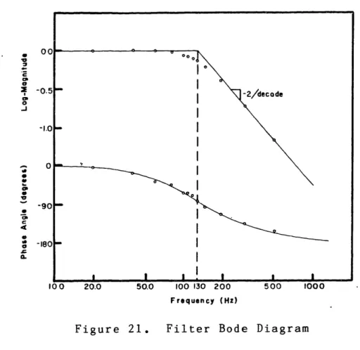
Measurement and 'Filter Model

The transducers needed to measure maximum moment and

loaded curvature will have a very large bandwidth compared to the servo system, so the dynamics of the measurements can be

ignored.

The signals must be filtered to eliminate

high-frequency noise from the transducer signals and reduce signal

aliasing. The amount of filtering necessary and the break

frequency of the filters will vary depending on the quality of the transducers, the required accuracy, the type of bending, and the sampling frequency In any case the filters can be modeled as a combination of first- and second-order differential equations. The filters used on all of the

experimental transducers are second-order Butterworth filters

with a break frequency of 130 Hz. Figure 21 shows the

fre-quency response of the filters.

The response is

second-order and can be modeled using Equation 12 with C = 0.707 and

w = 820 rad/sec.

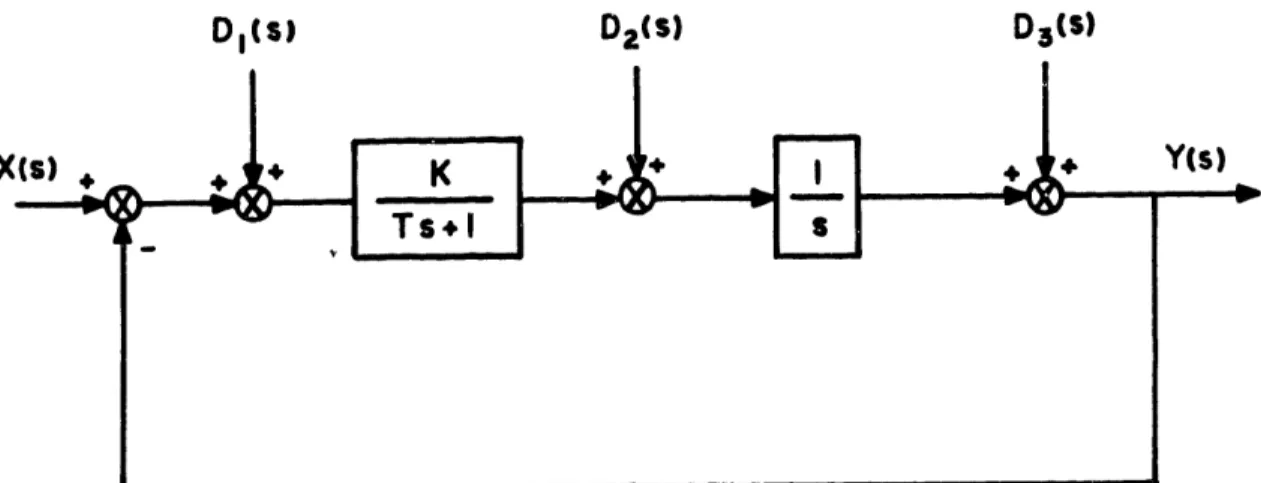
Disturbance Model

Disturbances in the system such as initial curvatures in

the workpiece can be modeled as a shift of the

moment-z .0CO a 0 0 -j I. 0 C 4 U1 Ca Frequency (Hz)

Figure 21. Filter Bode Diagram

curvature curve, as shown in Figure 7. This shift is incor-porated into the workpiece model by changing the yield point as shown in Figure 22. The disturbance curvature causes a change in the unloaded curvature which is exactly equal to the disturbance curvature. This is shown as a direct addi-tion in Figure 22. The shift in the yield point is deter-mined by applying Equation 16. This is modeled as an addi-tive term in Figure 22 which affects the input to the work-piece model. Equation 28 is the combined model for the

workpiece and curvature disturbance. This is the method used

in the simulation program listed in Appendix 4. Figure 23 is a plot of scaled moment, loaded curvature, and unloaded

Disturbance

I

Kd

+

Ku

Figure 22.

Disturbance Model Block Diagram

0 1 2 3 4 5 8 7 8 9 10

E-01

TIME (SEC)

Figure 23. Disturbance Detection

Zy

z

+

E-03 60 45

z

-i 30 15 0 -15

curvature as a workpiece which has an initial bend is

straightened by the experimental bending apparatus.

This

figure shows how the initial curvature disturbance is

detected by the closed-loop control scheme. Detection of the disturbance indicates that the disturbance is within the

control loop, which means that the disturbance can possibly

be eliminated with an appropriate controller. Notice that

there is an apparent shift between the moment and the loaded curvature in Figure 23. From Figure 3 it would seem that such a shift is impossible because any change in the moment requires a corresponding change in the curvature. But this is true only if the workpiece has a constant initial curva-ture, which means that the origin of the moment-curvature

relationship

is stationary.

If the initial curvature

changes, then the moment-curvature curve shifts as in Figure

7. This shift can be described as a change in curvature (from zero to some initial curvature) without a change in moment (unloaded in both cases), thus the apparent shift.

Figure 23 indicates a change in moment without a change in

curvature. This is because of the geometry of the roll

bending apparatus which causes the apparatus to sense the

disturbance in the moment measurement rather than the

curva-ture measurement. As stated earlier, the curvature is a very

strong function of center-roll position. In fact the loaded

curvature measurement in Figure 23 is actually proportional

to center roll position as given in Equation 16. When a flat

workpiece which contains a kink is rolled through the bending

apparatus, the following is observed. As the kink reaches the input roll and begins to enter the system, the workpiece tends to straighten because the rolls are initially stationary, and the curvature of the workpiece tends to

remain constant. The moment however, changes to reflect the

occurrence of the disturbance. This situation corresponds to

Point A in Figure 7 and to the first 0.1 sec in Figure 23. As the moment increases more than the curvature, the system

responds to eliminate the disturbance. This corresponds to

the response shown in Figure 23 up to 0.6 sec, where the

system has nearly reached steady state. This example

demon-strates that the closed-loop roll bending system will always

detect curvature disturbances with the moment measurement.

Controller Model

A specific controller model will be developed in the

next chapter, but the general form of the controller is given here. One important feature of the controller that must be taken into account if the controller is to be implemented by a digital computer, is the discrete nature of the control

signal. Even though the mechanical system is a continuous

system, the control signal from the computer will change only

at discrete intervals. This discretization can be modeled by

a zero-order hold equivalence. This model assumes that the

control signal is held constant over each interval until

updated at the next sampling time as shown in Figure 24.

Using Laplace transform notation the zero-order hold (ZOH)

can be described by:

-TS e

ZOH = 5

(20)

where T is the time in seconds of the interval between control signals and s is a complex variable defined in the

Laplace operator. For the computer and controllers used with

the experimental apparatus,

T

varied from 0.009 to 0.012

depending on the amount of computation required by the

controller.

-O 0. -

0

c

40-C

0

0

sO O

screte

T

2

3

4

5

6

7

8

9t

Time

Chapter 4

CONTROL

The models developed in Chapter 3 indicate that the roll

bending system is very much like a standard servo system.

The servo is the major component of the system and contains most of the significant dynamics. If the non-zero portion of Equation 17 is a perfect description of the relationship between servo movement and unloaded curvature, and if all the

parameters are known exactly, then the roll bending control

design nearly reduces to a standard servo controller.

But

the details of the servo/workpiece interaction introduce

unique dynamic effects which require more detailed analysis

than the standard servo control problem. In particular, the

deadband region represented by the zero portion of Equation

17 and the presence of disturbances in the form of initial

curvature are unique properties of the roll bending system.

Although the workpiece model is nonlinear, there is some

insight to be gained from a linear control analysis. If the workpiece can be described as a variable gain, then a linear

analysis should indicate the general form of the system

response to a specific controller. For this reason the roll

bending system will first be analyzed using linear control

techniques. These techniques are well known and will be used

without derivation (see for instance [25] or [26]). The control schemes suggested by this analysis will then be

eval-uated by using a computer simulation of the roll bending

system which includes the nonlinear workpiece model and the

discrete controller. This nonlinear control analysis should

produce a more realistic simulation of the actual system

response.

Control Objecti'es

The feasibility of closed-loop control of the roll

bending operation has been demonstrated using rudimentary

control in [18], [20], and [21]. The purpose of the control analysis in this chapter and the experiments described in Chapter 5 is to determine, if possible, the ultimate limits

of the roll bending system response and the practical factors

unique to the roll bending process that limit the response.

The control objective is to determine what control scheme or

schemes can be used to attain this ultimate response. The

problem is defining "ultimate response", because on a

practi-cal level the required system response will vary depending on the type of bending, part shape, feedrate, and error toler-ance. The control objective can be stated in general terms,

however, with individual objectives taking on more or less

importance for a specific application. To compare the

vari-ous control schemes the following control criteria will be

used to evaluate system response.

1) Stable system

roll bending system is always stable.

There are several

areas of particular concern. First, the nonlinearities cause

stability problems. Because the workpiece is a variable gain

dependent on bending stiffness and servo position, a control

scheme that is stable for a particular workpiece and bending

condition might not be stable for different workpieces and

conditions. Second, unmodeled dynamics can cause instability

if the system bandwidth is large enough. There are unmodeled

dynamics in all components, but particularly in the servo

system and workpiece. The servo system has unmodeled

dynam-ics associated with friction, backlash, and compliance in the

coupling between the DC motor and the ballscrew. The work-piece is modeled as a variable gain, but actually contains

mass, compliance, and damping.

These unmodeled workpiece

dynamics are especially troublesome as shown in Chapter 5.

2) Zero steady-state error

This objective is very important for straightening

applications or for other types of bending where a high

degree of accuracy is required.

Steady-state error is

generally associated with a particular input. The

steady-state error properties of the control schemes developed in

this chapter will be evaluated in response to a step input. Linear control theory shows that a free integrator in the

open-loop transfer function (Type I system) is enough to

guarantee zero steady-state error to a step input. Note that

a free integrator does not necessarily guarantee zero

steady-state error in response to system disturbances, depending on where the disturbances enter the system in relation to the

integrator.

This becomes important for the straightening

operation, since initial curvature is a disturbance to the

closed-loop roll bending system.

3) High bandwidth

The high bandwidth criterion is really a measure of how well the system can follow a command. The required bandwidth of the system is determined largely by the frequency content of the input command and the disturbances. For the roll bending system the input command and the disturbances are in the form of curvature as a function of the distance along the

workpiece.

In other words the input commands and

distur-bances have a constant spatial frequency, but the time fre-quency is variable depending on the feedrate. For example,

consider a workpiece that contains an initial curvature that

is a sine wave of unit amplitude and 1.0 cycle/ft of length

frequency along the workpiece.

If the workpiece is rolled

through the bending apparatus using a feedrate of 1.0 ft/sec,

then the controller will measure a disturbance which has a frequency of 1.0 cycle/sec. If the same workpiece is rolled through the apparatus using a feedrate of 2.0 ft/sec, then the disturbance seen by the controller is at a frequency of

2.0 cycle/sec. This shows that the feedrate actually