A methodology for physically based rockfall hazard assessment

HAL Id: hal-00301598

https://hal.archives-ouvertes.fr/hal-00301598

Submitted on 1 Jan 2003

HAL is a multi-disciplinary open access

archive for the deposit and dissemination of

sci-entific research documents, whether they are

pub-lished or not. The documents may come from

teaching and research institutions in France or

abroad, or from public or private research centers.

L’archive ouverte pluridisciplinaire HAL, est

destinée au dépôt et à la diffusion de documents

scientifiques de niveau recherche, publiés ou non,

émanant des établissements d’enseignement et de

recherche français ou étrangers, des laboratoires

publics ou privés.

assessment

G. B. Crosta, F. Agliardi

To cite this version:

G. B. Crosta, F. Agliardi. A methodology for physically based rockfall hazard assessment. Natural

Hazards and Earth System Science, Copernicus Publications on behalf of the European Geosciences

Union, 2003, 3 (5), pp.407-422. �hal-00301598�

c

European Geosciences Union 2003

and Earth

System Sciences

A methodology for physically based rockfall hazard assessment

Universit`a degli Studi di Milano-Bicocca, Piazza della Scienza, 4, I-20126 Milano, Italy Received: 9 September 2002 – Accepted: 21 November 2002

Abstract. Rockfall hazard assessment is not simple to achieve in practice and sound, physically based assessment methodologies are still missing. The mobility of rockfalls implies a more difficult hazard definition with respect to other slope instabilities with minimal runout. Rockfall haz-ard assessment involves complex definitions for “occurrence probability” and “intensity”. This paper is an attempt to eval-uate rockfall hazard using the results of 3-D numerical mod-elling on a topography described by a DEM. Maps portray-ing the maximum frequency of passages, velocity and height of blocks at each model cell, are easily combined in a GIS in order to produce physically based rockfall hazard maps. Different methods are suggested and discussed for rockfall hazard mapping at a regional and local scale both along lin-ear features or within exposed areas. An objective approach based on three-dimensional matrixes providing both a posi-tional “Rockfall Hazard Index” and a “Rockfall Hazard Vec-tor” is presented. The opportunity of combining different parameters in the 3-D matrixes has been evaluated to bet-ter express the relative increase in hazard. Furthermore, the sensitivity of the hazard index with respect to the included variables and their combinations is preliminarily discussed in order to constrain as objective as possible assessment cri-teria.

1 Introduction

Rockfalls are the among the most common landslide types in mountain areas. Despite usually involving limited vol-umes (Rochet, 1987), rockfalls are characterised by high en-ergy and mobility, making them a major cause of landslide fatalities (Guzzetti, 2000). Rockfalls can be triggered by earthquakes (Kobayashi et al., 1990), rainfall or freeze-and-thaw cycles (Matsuoka and Sakai, 1999) or the progressive weathering of rock material and discontinuities in suitable Correspondence to: G. B. Crosta

(giovannib.crosta@unimib.it)

climatic conditions. They originate from cliffs of different sizes (from few metres to hundreds of metres high) and na-tures (lithologic, structural, etc.), and involve a wide range of volumes (Rochet, 1987; Hungr and Evans, 1988). Rock-falls are among the most destructive mass movements, and pose a severe threat to humans, properties and utilities where they occur (Cancelli and Crosta, 1993; Bunce et al., 1997). For these reasons rockfall hazard and risk assessment are of major interest to technicians, administrators and local plan-ners (Cancelli and Crosta, 1993; Fell, 1994; Fell and Hart-ford, 1997; Crosta and Locatelli, 1999; Guzzetti et al., 1999). Rockfall hazard assessment is not simple to achieve in prac-tice and sound, physically based assessment methodologies are still missing.

Despite the fact that rockfalls are common, few attempts have been made to evaluate the related hazard, and the as-sociated risk, in a spatially distributed way (Van Dijke and Van Westen, 1990; Cancelli and Crosta, 1993; Crosta and Locatelli, 1999; Wieczorek et al., 1999), or along transporta-tion or utility corridors (Evans and Hungr, 1993; Bunce et al., 1997; Hungr at al., 1999). Most of the available haz-ard assessment methods are empirical (Pierson et al., 1990; Dussauge-Peisser et al., 2002) or semi-empirical (Cancelli and Crosta, 1993; Rouiller and Marro, 1997; Crosta and Lo-catelli, 1999). They often consider only the onset (or trigger-ing) probability of rockfalls, without any characterisation or modelling of rockfall trajectories in 2-D or 3-D. This leads to a subjective definition and zonation of rockfall hazard, mak-ing the validation and comparison of different methodologies difficult (Mazzoccola and Sciesa, 2000; Interreg IIC, 2001).

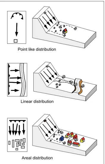
This paper presents a physically-based procedure to eval-uate rockfall hazard using the results of 3-D numerical mod-elling, performed through an original simulation code. Com-puting rockfall trajectories is mandatory to achieve objec-tive rockfall hazard assessment. In addition, the use of 3-D modelling is fundamental to face different classes of haz-ard problems (Crosta and Locatelli, 1999), namely Fig. 1: point-like (single elements, small areas), linear or corridor-like (lifelines, routes) and areal (urban areas, areas subjected

Point like distribution

Linear distribution

Areal distribution

Fig. 1. Different categories of rockfall hazard problems.

to planning). These problems are characterised by increas-ingly difficult hazard assessment. In this study, the results of 3-D rockfall models performed at both regional and local scales, have been used to test the method on areal and linear problems. The use of 3-D matrixes providing a positional “Rockfall Hazard Index” and a “Rockfall Hazard Vector” is presented and discussed. Furthermore, the sensitivity of haz-ard maps to the included variables and their combination is discussed in order to constrain the assessment criteria as ob-jectively as possible.

2 Numerical modelling of rockfalls

Rockfall phenomena start by the detachment of blocks from their original position. This phase is followed by free falling, bouncing, rolling or sliding (Broili, 1973; Varnes, 1978; Boz-zolo and Pamini, 1986), with falling blocks losing energy at impact points or by friction. Kinematic, dynamic or empir-ical equations (Falcetta, 1985; Bozzolo and Pamini, 1986; Descouedres and Zimmerman, 1987; Rochet, 1987; Bozzolo et al., 1988; Pfeiffer and Bowen, 1989; Evans and Hungr,

1993; Wieczorek et al., 1999) can be used to model rockfall processes and define regions subjected to this hazard.

Rockfall dynamics is a complex function of the location of the detachment point and the geometry and mechanical prop-erties of both the block and the slope. Theoretically, knowing the initial conditions, the slope geometry, and the relation-ships describing the energy loss at impact or by rolling, it should be possible to compute the position and velocity of a block at any time. Nevertheless, relevant parameters are diffi-cult to ascertain both in space and time, even for an observed event. Usually, the geometrical and geomechanical proper-ties of the blocks (size, shape, strength, fracturing) and of the slope (gradient, length and roughness, longitudinal and transversal concavities and convexities, grain size distribu-tion, elastic moduli, water content, etc.), and the exact loca-tion of the source areas are unknown. The same can be said for the variability of the controlling parameters. In addition, the energy lost at each impact or during rolling depends on a variety of factors including the velocity of the block and the impact angle, the block to slope contact type (block cor-ner, edge or face), and the presence and density of vegetation (Bozzolo and Pamini, 1986; Cancelli and Crosta, 1993; Az-zoni and De Freitas, 1995; Jones et al., 2000). These param-eters are difficult to quantify both precisely and accurately at any spatial scale. Thus, “contact functions” relating the block kinematics (in terms of velocity) or dynamics (in terms of en-ergy) before and after the impact, are introduced to model the energy loss at each impact point. Such functions are usually expressed as restitution and friction coefficients and regarded as material constants even if, as already mentioned, they in-clude the effects of many different controlling factors (type and thickness, texture and structure of slope deposits, block size and geometry, angle and velocity of impact, geometry of the impact, vegetation, soil moisture content, etc.).

When rockfall trajectories are computed along a limited number of 2-D slope profiles defined a priori, the interpre-tation of the results and its extension to neighbouring areas may not be straightforward (or unique), and require exten-sive engineering judgment in order to be used for hazard as-sessment purposes (Crosta and Locatelli, 1999). In fact, the three-dimensional nature of actual slope geometry (e.g. the presence of chutes and channels, convexities and longitudi-nal ridges), strongly affect the trajectories and the partition of kinetic energy into translational and rotational components (Chau et al., 2002). Different computer codes and algorithms have been proposed (Bozzolo and Pamini, 1986; Descoue-dres and Zimmermann, 1987; Bozzolo et al., 1988; Evans and Hungr, 1988; Pfeiffer and Bowen, 1989; Azzoni et al., 1995; Stevens, 1998; Jones et al., 2000), but few 3-D models have been developed (Descouedres and Zimmermann, 1987; Guzzetti et al., 2002). Available software performs 2-D or 3-D simulations using a kinematic (i.e. lumped-mass), a dy-namic, or a “hybrid” (i.e. kinematic for free fall and dynamic for impact and/or for rolling) approach (Crosta and Agliardi, 2000). Tools are also provided to cope with the variabil-ity of input data (Bozzolo and Pamini, 1986; Descouedres and Zimmermann, 1987; Pfeiffer and Bowen, 1989; Scioldo,

1 2 3 1 2 3 1 2 3 RHI = (232) ½RHV = 4.123½ c h k 333 232 1 2 3 1 2 3 1 2 3 a) b) c) h h c c k k

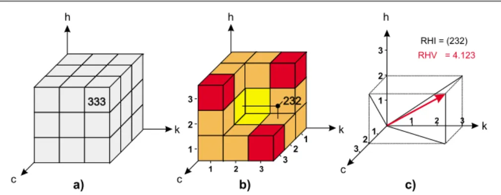
Fig. 2. The three-dimensional matrix ckh, used for rockfall hazard assessment. (a) General definition of the positional Rockfall Hazard

Index, RHI; (b) splitted matrix cube with ranked RHI values; (c) Rockfall Hazard Vector (RH V ) concept.

1991; Azzoni et al., 1995; Stevens, 1998; Jones et al., 2000). Keeping in mind the aforementioned problems, we de-signed and developed an original rockfall simulation pro-gram, named STONE (Agliardi et al., 2001; Agliardi and Crosta, 2002; Guzzetti et al., 2002; Agliardi and Crosta, 2003). The program computes rockfall trajectories in 3-D, and allows one to prepare spatially distributed maps of the frequency and kinematics of rockfalls. The code has some specific characteristics concerning the modelling approach and the preparation of input data, namely:

– a lumped mass algorithm allows modelling free fall,

im-pact and rolling motions in a 3-D framework;

– topography is provided as a Digital Elevation Model

(DEM), without resolution restrictions, and a vector to-pography is recalculated starting from the DEM;

– spatially distributed input data are provided, without

limitations to the number of land units introduced to de-scribe surface lithology and land use;

– rockfall sources can be defined as points, lines or

poly-gons; a different number of blocks can be launched from each source cell, allowing simulating different on-set probabilities of rockfalls;

– stochastic modelling through a “pseudo-random”

ap-proach can be performed and repeated;

– air drag and block fracturing are not taken in account

for simplicity;

– the program accepts input data and produces outputs in

a raster EsriTM GridAscii format, allowing for integra-tion with GIS environments for pre- and post-processing of input data and model results.

STONE requires the following input data:

– a raster grid containing elevation data (DEM);

– a grid of the source cells and of the number of boulders

to be launched from each cell;

– three grids containing the values for the normal and

tan-gential restitution coefficients and the rolling friction coefficient;

– a parameter file specifying the input filenames and the

main controlling parameters and variability.

The following 2-D-raster and 3-D-vector outputs are pro-vided:

– raster maps which portray at each cell: the cumulative

count of rockfall transits; the maximum computed ve-locity; and the largest flying height;

– vector outputs which provide instantaneous velocity and

fly height at each sampled point of the computed fall paths.

As above mentioned, STONE allows for the inherent nat-ural variability of the input data to be taken in account by launching a variable number of blocks from each detachment cell. This can simulate both a different zone-by-zone onset probability of rockfalls and the stochastic nature of the rock-fall process. The initial projection angle, the dynamic rolling friction coefficient, and the normal and tangential restitu-tion coefficients can be varied randomly within pre-defined ranges for each of the multiple launched blocks. In order to consider the dependence of the restitution coefficients on block mass and velocity, a couple of semi-empirical relation-ships (Pfeiffer and Bowen, 1989; Stevens, 1998) have been implemented in the code. Consequently, the normal and tan-gential restitution coefficients can be scaled according to the imposed block mass or the computed impact velocity. No de-pendence of the normal restitution coefficient on the impact angle has been introduced in the code at this moment.

3 Physically-based rockfall hazard assessment

3.1 Suitable strategies

Rockfall modelling aims to define, for a specified “design block”, the fall path, the maximum runout distance, the en-velope of trajectories and the velocity and energy distribution

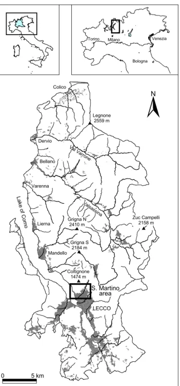
S. Martino area Val Varrone Valsassina Colico Dervio Bellano Varenna Lierna Mandello LECCO Lake of Como Legnone 2559 m Grigna N 2410 m Grigna S 2184 m Coltignone 1474 m Zuc Campelli 2158 m $ $ $ # $ $ Milano Torino Venezia Bologna N 5 km 0

Fig. 3. Location map of the study areas in the Lombardy re-gion (northern Italy): the Lecco Province and the Mt. S. Martino-Coltignone area.

along them. This information results in rockfall hazard and risk assessment, and in the design and planning of counter-measures (Spang, 1987; Cancelli and Crosta, 1993; Crosta and Locatelli, 1999). In engineering practice, these studies are usually performed along specific 2-D slope profiles.

Landslide hazard has been usually defined in the litera-ture as the probability of occurrence of a landslide of given magnitude, in a pre-defined period of time, and within a given area (Varnes et al., 1984; Fell, 1994; Fell and Hartford,

1997; Guzzetti et al., 1999; Crosta et al., 2001). This defini-tion incorporates the concepts of spatial locadefini-tion, magnitude and frequency of occurrence of a landslide. Spatial location refers to the ability to forecast where a landslide will occur; magnitude refers to the prediction of the geometrical and me-chanical intensity (i.e. the amount of energy involved), and frequency refers to the forecasting of the temporal recurrence of the landslide event (Varnes, 1984; Einstein, 1988). Thus, the simplest rockfall hazard map should portray the prob-ability of occurrence of rockfalls of pre-defined magnitude within a given area.

The high mobility of rockfalls (as is the case with debris flows and rock avalanches) implies a major difference in haz-ard assessment with respect to other slope instability phe-nomena characterised by minimal expansion. The local re-currence probability for high mobility phenomena must de-rive from the detachment and the transit components (Can-celli and Crosta, 1993; Crosta and Locatelli, 1999; Interreg IIC, 2001), both of which vary in space, along the same tra-jectory and moving laterally to another one. Furthermore, rockfall intensity must be evaluated along each rockfall path. As a consequence, rockfall hazard can be better defined as the probability of occurrence (including detachment and transit) of a rockfall of given magnitude, in a pre-defined pe-riod of time and at any location along a slope susceptible to its transit.

The definition of hazard introduced above involves an in-creased level of information needed for objective hazard as-sessment. In fact, it is not enough to know the total runout length and the associated probability to reach this maximum distance. Elements at risk can be located at different dis-tances along the rockfall path. Thus, the intensity and prob-ability of rockfall occurrence at a given location must be defined along the entire falling path. Since probability and intensity vary along the slope as complex functions of the mechanical and geometrical characteristics of both the slope and the falling blocks, this definition calls for a physically sound modelling of rockfall motion along a slope. The local occurrence probability derives from the combination of the onset probability (related to the geomechanical susceptibility of rock masses to fail) and the transit or impact probability at a given location (related to the motion of falling blocks). Rockfall intensity is a complex function of mass, velocity or energy and fly height of blocks. Thus, the intensity can be defined in different ways depending on the adopted physical description and destructiveness criterion.

The raster or vector maps prepared by STONE outline the areas where rockfalls are expected to occur and their kine-matic features. Thus, they are likely to be combined to pro-vide a spatial assessment of rockfall hazard (Agliardi et al., 2002). The count of rockfall trajectories is a proxy for the probability of occurrence of rockfalls. At any cell, the map portrays the chance of being crossed by a rockfall trajectory, resulting from the number of launched blocks, the variability of the controlling parameters, the local morphology and the DEM detail. The maximum computed rockfall velocity and fly height provide separate information on rockfall intensity

to be associated with the block design mass. A distributed set of block mass values can be inserted in the model for a translational kinetic energy-based computation of the inten-sity.

Two main questions arise. First, what is the best way to compute and represent hazard? Second, how can different hazard levels be ranked? According to our approach, rock-fall hazard can be derived by the combination of different in-dependent components, depending on the adopted definition of intensity. For example, hazard could be function of three, equally important components, one probabilistic (count, c) and two kinematic (velocity, v, and fly height, h). One more option consists in the use of the rockfall count (c), the com-puted translational kinetic energy (k) and the fly height (h). In this way, rockfall dynamics is introduced by means of k. The fly height could be eventually considered as a weak in-dicator of hazard level. This is because it is relevant only for prediction of impact on elements of different vertical size or on the influence on down-slope located points. As a conse-quence, hazard could be a function of the count (c) velocity (v) and the mass (m).

We have introduced a “dynamic” component in rockfall hazard assessment by considering hazard as a function of the computed rockfall count (c), kinetic energy (k) and fly height (h). The three components are conveniently represented in a 3-D space, by defining a 3-D matrix which portrays hazard as a function of the adopted parameters (Fig. 2).

The rockfall hazard conditions defined by the 3-D matrixes can be expressed using a “Rockfall Hazard Index” (Fig. 2) defined as RHI = (ckh). The digits of the RHI are reclassi-fied values of the adopted variables. The RHI has a positional meaning, i.e. hazard is identified by a specific position in the hazard parameter space. The approach is affected by some conceptual problems. Are all the possible values of RHI re-alistic? How can RHI values be ranked to define the hazard level and perform zonation? As to the first question, if the values of the controlling parameters (for example c, k, and

h) are ranked into n classes (0 to n, in order to allow for combination into a 3-digit index), RHI = (000) will corre-spond to the origin of the 3-D hazard space, representing a condition where rockfalls are not expected. In a similar way, any RHI value including a zero digit is unrealistic since it indicates no rockfall occurrence, and the lowest acceptable RHI digit value is 1. As to hazard ranking (Fig. 2), rockfall hazard increases at a maximum rate along the diagonal line that trisects the hazard space. Other RHI values represent intermediate hazard conditions. From a purely geometrical point of view, all the points lying on planes perpendicular to the diagonal line should exhibit the same hazard level. Actu-ally, since the input parameters are reclassified into discrete classes, the hazard index is also discrete. In addition, many different real situations could be outlined on a “constant haz-ard” plane, involving different occurrence probabilities and different amount of kinetic energy and, thus, requiring differ-ent mitigation approaches. The use of a positional index al-lows one to keep track of the contribution of each variable to the hazard and, thus, to outline “why” a location on the slope

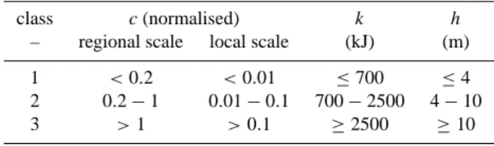
Table 1. Parameter reclassification scheme used in the Rockfall

Hazard Index/vector procedure. Note that the values of c are nor-malised according to different approaches depending on the mod-elling scale. See text for explanation

class c(normalised) k h

– regional scale local scale (kJ) (m)

1 <0.2 <0.01 ≤700 ≤4

2 0.2 − 1 0.01 − 0.1 700 − 2500 4 − 10

3 >1 >0.1 ≥2500 ≥10

is characterised by a given hazard level. Nevertheless, the po-sitional nature of the RHI index hampers the direct ranking of hazard. For example (Fig. 2), it will be difficult to decide if RHI = (113) portrays a higher hazard than RHI = (311) or RHI = (121). Thus, the RHI index needs to be translated into a sequential one. Thus, we will introduce the concept of Rockfall Hazard Vector (RH V ), its magnitude to be used as hazard ranking criterion (Fig. 2). The hazard vector approach can be figured as an “onion skin” approach, with increasing hazard level moving outward.

3.2 Rockfall Hazard Index/Vector procedure

The effectiveness of a hazard map relies on different ele-ments. First, a physically based modelling approach is con-sidered fundamental, because it allows for an accurate de-scription of rockfall phenomena and decreases the amount of engineering judgement required. Accuracy of the input data is another major element controlling the quality of the hazard maps. Finally, practical efficacy of hazard maps also depends on their clarity, i.e. on the fragmentation of the in-formation provided. In fact, a useful hazard map should por-tray as many as possible different areas homogeneous with respect to hazard, allowing decision makers to optimise land planning. Nevertheless, excessive fragmentation of the in-formation provided by the map could be misleading when planning urban development. For example, small “safe” iso-lated areas in a generally “unsafe” area could be not suitable for developing in practice.

Starting from the aforementioned considerations, we de-veloped a new rockfall hazard assessment procedure: this is conceived to take in account as many physical aspects of rockfall as possible, to be easy to use and to provide mean-ingful hazard maps, to be translated into planning tools with little further effort. The method considers three main param-eters which are computed directly or indirectly by STONE, namely: the rockfall count c, the translational kinetic energy

k =0.5 m v2, and the fly height h. According to the method, rockfall hazard is expressed by a “Rockfall Hazard Index” RHI = (ckh).

Since the three parameters are characterised by different physical meanings and orders of magnitude, their values are conveniently reclassified in three classes. The choice of a

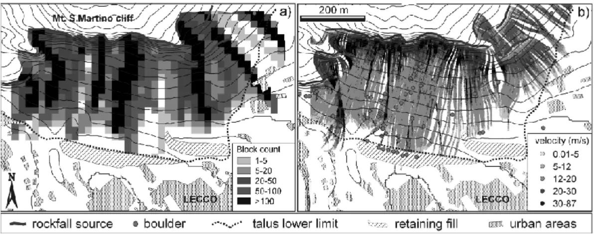
Fig. 4. Close up of the Mt. S. Martino cliff area (north of Lecco urban area). Model results obtained at different scale and data format are

shown: (a) raster map of the rockfall count, obtained from the regional scale model of the Lecco Province (20 m ground resolution DEM); (b) vector trajectories, classified by velocity, obtained from the local-scale model of the Mt. S. -Coltignone area (5 m ground resolution DEM).

small number of classes allows us to simplify the classifica-tion and ranking of the computed RHI values (i.e. a 3 class subdivision results in 27 RHI values) and to obtain clearer hazard maps. The classification and ranking of the factors contributing to hazard is an intrinsically uncertain task, usu-ally performed on a subjective basis. In order to overcome this problem at least partially, the three controlling parame-ters are classified according to standard criteria, established through the objective evaluation of the “potential destructive-ness” of simulated rockfalls. Hazard assessment is usually performed for planning or mitigation purposes. From this point of view, an increasing kinetic energy implies higher ca-pability of a falling rock of damaging structures (i.e. build-ings, infrastructure, etc.) and passive countermeasures (e.g. barriers). In addition, higher maximum fly height results in higher probability for barriers to be overcome or for higher structures to be hit. According to these considerations, we decided to reclassify the parameters c, k and h according to a scheme (Table 1) directly related with the possible final use of hazard maps for mitigation purposes.

The range of computed values of translational kinetic en-ergy k is reclassified in three classes. Class intervals corre-spond to the maximum energy absorption capacity of com-mon types of rockfall barriers, namely: elastic catch nets sorbable energy up to 700 kJ) and elasto-plastic barriers (ab-sorbable energy up to 2500 kJ). The basic idea is that more hazardous rockfalls are able to damage more effective bar-rier typologies. This also conveys in the final hazard map useful information for hazard reduction through countermea-sure design. Thus, classes 1, 2 and 3 will be defined for 0 < k ≤ 700 kJ, 700 < k ≤ 2500 kJ and > 2500 kJ, re-spectively. In the last ten years, advances in material science and barrier technology has brought new barrier types, char-acterised by higher capacity. Nevertheless, we found that the proposed values are representative of the most used passive countermeasures in the Italian alpine area. In a similar way, rockfall fly height h is reclassified according to the ability of

a rockfall to overcome specific types of passive countermea-sures, namely: catch nets (h = 4 m) and retaining fills (h up to 10 m). In this case classes 1, 2 and 3 will be defined for 0 < h ≤ 4 m, 4 < h ≤ 10 m and h > 10 m, respectively. The zero value for the parameter h is included in the class 1, differently from the kinetic energy. In fact, a value of 0 kJ means no rockfall occurrence (or a stopped rockfall), while a fly height of zero means that the block is impacting or rolling. Eventually, class limits for k and h can be redefined by users involved in rockfall analysis in different geomorphological or engineering settings and practice standard, if information concerning the existing structures (heights of buildings) and countermeasures (heights and capacities of barriers; Gerber, 2001) are available. Nevertheless, the reclassification criteria should be retained if this method is used.

The reclassification of the rockfall count is more diffi-cult, since unique meaningful class boundaries in the rock-fall count do not exist. In fact, the number of blocks pass-ing through a model cell depends on the topography and the number of launched blocks, and strongly varies on a case-by-case basis. Thus, we propose to reclassify count values normalised according to two different approaches, depend-ing on whether the modelldepend-ing is performed at a regional or at a local scale (Table 1).

For regional scale models, characterised by a very large number of launched blocks (e.g. up to 1 million or more), the rockfall count is normalised by a specific approach. We know that most hazardous areas are associated to the max-imum probability of rockfall occurrence, and that rockfall frequency on a channelled topography is significantly higher than that on simple planar slopes. Thus, rockfall count values can be normalised with respect to standard values represent-ing the transition from planar to channelled morphologies. We assume that at least 5 “contributing” cells, located in a C-shaped pattern, are needed to initiate a channel effect on a given cell. This corresponds to the transition from a pla-nar to a channelled morphology. A number of 5 contributing

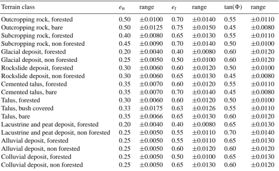
Table 2. Calibrated average values and variability ranges of the restitution and friction coefficients for the Lecco Province rockfall model.

The different terrain classes have been obtained by “unique condition” combination of surface lithology and land use

Terrain class en range et range tan(8) range

Outcropping rock, forested 0.50 ±0.0100 0.70 ±0.0140 0.55 ±0.0110

Outcropping rock, bare 0.50 ±0.0125 0.75 ±0.0150 0.45 ±0.0080

Subcropping rock, forested 0.40 ±0.0080 0.65 ±0.0130 0.55 ±0.0110

Subcropping rock, non forested 0.45 ±0.0090 0.70 ±0.0140 0.50 ±0.0100

Glacial deposit, forested 0.20 ±0.0040 0.40 ±0.0080 0.60 ±0.0120

Glacial deposit, non forested 0.25 ±0.0050 0.50 ±0.0100 0.60 ±0.0120

Rockslide deposit, forested 0.30 ±0.0060 0.60 ±0.0120 0.50 ±0.0100

Rockslide deposit, non forested 0.30 ±0.0060 0.65 ±0.0130 0.45 ±0.0080

Cemented talus, forested 0.35 ±0.0070 0.60 ±0.0120 0.55 ±0.0110

Cemented talus, bare 0.35 ±0.0070 0.70 ±0.0140 0.45 ±0.0080

Talus, forested 0.30 ±0.0060 0.60 ±0.0120 0.50 ±0.0100

Talus, bush covered 0.33 ±0.0175 0.63 ±0.0126 0.55 ±0.0110

Talus, bare 0.35 ±0.0066 0.65 ±0.0130 0.60 ±0.0120

Lacustrine and peat deposit, forested 0.20 ±0.0040 0.40 ±0.0080 0.65 ±0.0130

Lacustrine and peat deposit, non forested 0.25 ±0.0050 0.55 ±0.0110 0.70 ±0.0140

Alluvial deposit, forested 0.25 ±0.0050 0.55 ±0.0110 0.65 ±0.0130

Alluvial deposit, non forested 0.25 ±0.0050 0.60 ±0.0120 0.60 ±0.0120

Colluvial deposit, forested 0.25 ±0.0050 0.50 ±0.0100 0.65 ±0.0130

Colluvial deposit, non forested 0.25 ±0.0050 0.65 ±0.0130 0.60 ±0.0120

cells is a lower bound value for channelling, assuming that other contributing cells (e.g. from rockfall sources placed above on the slope) are ignored. According to this approach, the rockfall count (c) at any given transit cell is normalised with respect to the number (5 ∗ n) of launched blocks from each group of 5 contributing source cells (n is the number of blocks launched from each cell). Thus, for the transition from planar to channelled slopes (5 contributing cells) and, for example, for n = 1, the count is c = 5 and the nor-malised count value will be c/(5 ∗ n) = 1. On the opposite, for a rectilinear source area corresponding to a planar slope (1 contributing cell), for n = 1 the count is c = 1 and the normalised count will be c/(5 ∗ n) = 0.2. This approach allows to normalise the count by describing implicitly also the relative size of the contributing area. Normalised count values less than 0.2 will denote low rockfall frequency in un-channelled areas. Values ranging from 0.2 to 1 will denote increasing rockfall frequency on relatively simple slopes. Fi-nally, values higher than 1 will identify the most hazardous areas with respect to rockfall frequency (e.g. areas charac-terised by convergence of trajectories or very high rockfall frequency on planar slopes). The approach provides a way to reclassify the count independent on the actual count value, which can be a weak indicator itself.

For local scale models, where the geomechanical features of localised source areas are better known, we normalised the rockfall count with respect to the total number of launched blocks from a single homogeneous area (i.e. characterised by uniform size, mass and frequency of launched blocks). The two main reasons for this different approach are, namely: the need to compare the different hazard deriving from blocks

falling from homogeneous areas; the importance of main-taining separate the contributions given by blocks coming from different source areas but converging on the same in-vasion area. When homogeneous sub-areas are not defined, the rockfall count can be normalised according to the same criterion used at regional scale. For the local scale models, we propose to reclassify the normalised count values accord-ing to the followaccord-ing intervals: < 0.01, 0.01−0.1, > 0.1. We stress in any case the fact that different intervals can be cho-sen according to model outputs and the number of launched blocks.

Once the input parameters have been reclassified (Table 1), they are combined to obtain a value of the 3-digit positional Rockfall Hazard Index (RHI), portraying on the map a spe-cific level of hazard and retaining in each digit the informa-tion about the contribuinforma-tion of each parameter. The resulting 27 classes (Fig. 2a and b) are considered sufficient to rep-resent hazard but they are not easily reprep-resented in a map. Then, further regrouping is performed to result in 3 hazard classes (low, intermediate and high). This requires a ranking criterion allowing us to translate the positional index value into a sequential value. Such a criterion is provided by the magnitude of a Rockfall Hazard Vector (RH V ) (Fig. 2c), defined as: RH V =   c k h  , (1)

where c, k and h are the reclassified values of the input pa-rameters (i.e. RHI digits). The RH V magnitude is simply

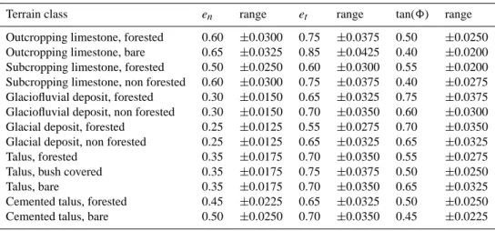
Table 3. Calibrated average values and variability ranges of the restitution and friction coefficients for the Mt. S. Martino-Coltignone area

rockfall model. The different terrain classes have been obtained by “unique condition” combination of surface lithology and land use

Terrain class en range et range tan(8) range

Outcropping limestone, forested 0.60 ±0.0300 0.75 ±0.0375 0.50 ±0.0250

Outcropping limestone, bare 0.65 ±0.0325 0.85 ±0.0425 0.40 ±0.0200

Subcropping limestone, forested 0.50 ±0.0250 0.60 ±0.0300 0.55 ±0.0200

Subcropping limestone, non forested 0.60 ±0.0300 0.75 ±0.0375 0.40 ±0.0275

Glaciofluvial deposit, forested 0.30 ±0.0150 0.65 ±0.0325 0.75 ±0.0375

Glaciofluvial deposit, non forested 0.30 ±0.0150 0.70 ±0.0350 0.60 ±0.0300

Glacial deposit, forested 0.25 ±0.0125 0.55 ±0.0275 0.70 ±0.0350

Glacial deposit, non forested 0.25 ±0.0125 0.65 ±0.0325 0.65 ±0.0325

Talus, forested 0.35 ±0.0175 0.70 ±0.0350 0.55 ±0.0275

Talus, bush covered 0.35 ±0.0175 0.75 ±0.0375 0.50 ±0.0250

Talus, bare 0.35 ±0.0175 0.70 ±0.0350 0.65 ±0.0325

Cemented talus, forested 0.45 ±0.0225 0.65 ±0.0325 0.50 ±0.0250

Cemented talus, bare 0.50 ±0.0250 0.70 ±0.0350 0.45 ±0.0225

given by:

|RH V | =pc2_+k2_+h2_{. (2)}

Since c, k and h are discrete, the vector magnitude is dis-crete, too. Nevertheless, the magnitude of the RH V vector allows us to rank the hazard level in classes and to obtain an objective and clear hazard map.

4 Example applications

The Rockfall Hazard Index/Vector method has been tested at different scales in two study areas in the Central Italian Alps (Lombardy, Northern Italy), namely: the Lecco Province and the Mt. S. Martino-Coltignone area (Fig. 3). For the former we performed a regional hazard assessment, whereas for the latter we ascertained rockfall hazard at the local scale. 4.1 Regional scale modelling: the Lecco Province

(Lom-bardia Region, Northern Italy)

The Lecco Province covers about 570 km2, mainly along the eastern shore of Como Lake (Fig. 3). Thinly bedded and massive limestone, dolostone, marl, sandstone and metamor-phic rocks (Crosta, et al., 2001) crop out. In this area, high and very steep rock slopes are frequent especially in lime-stone and dololime-stone. Rockfalls are also frequent, posing a severe threat to some urban areas and along roads and the railway running along Como Lake. Fatalities caused by rockfalls (Cancelli and Crosta, 1993; Crosta and Locatelli, 1999; Agostoni et al., 1999) have occurred in the area of Mt. S. Martino-Coltignone (February 1969, 8 casualties), at Valmadrera (July 1981, 1 casualty), at Onno Lario (1984, 1 casualty) and at Varenna (May 1997, 5 casualties).

A DEM with a ground resolution of 20 m was available for the entire area, obtained by interpolation of a subset of con-tour lines from the 1:10 000 scale topographic maps of the

Regione Lombardia. The source areas of rockfalls were as-certained from a landslide inventory map prepared by the Re-gione Lombardia and the Province of Lecco (Agostoni et al., 1999). About 57 km2of the whole territory (10% of the total area) have been mapped as a possible “source area of rock-falls”. These areas include rocky cliffs identified on 1:10 000 topographic maps and from stereoscopic aerial photos. Mi-nor unstable rock outcrops have been mapped through field surveys and historical rockfall reports, and 141 385 source cells were identified at the same ground resolution of the DEM. Since the experimental determination of the restitu-tion (normal and tangential) and dynamic rolling fricrestitu-tion co-efficients across large areas is impossible both for logistic and budget limitations, initial values for such coefficients were attributed by reclassifying a “unique condition map” obtained by overlaying information about surface lithology, slope deposits, landslides, and vegetation, in order to obtain homogeneous “land units” with respect to the restitution and friction characteristics. As a consequence, unique condition areas are sectors of the study area where different features (i.e. lithology, slope deposits, landslides, vegetation, land use, etc.) are present with the same attribute (e.g. limestone, blocks, no landslide, grass, pasture, etc.).

Table 2 shows the classes adopted in the unique condi-tion map, and the relative average calibrated values for the normal, tangential and rolling friction coefficients. Initial se-lection of the coefficients was based on data available in the literature (Crosta and Agliardi, 2000) for the same type of simulation approach. The range of values for each unique condition class has been calibrated according to the exten-sion of scree slopes, to historic rockfall events and to the lo-cation of major boulders along the slopes. This was the most time demanding phase of the whole study because of its sig-nificance on the final results (Agliardi and Crosta, 2002).

Rockfall modelling has been performed using a probabilis-tic approach, by throwing 10 blocks from each source cell (for a total of 1 413 850 launched blocks) and allowing for the

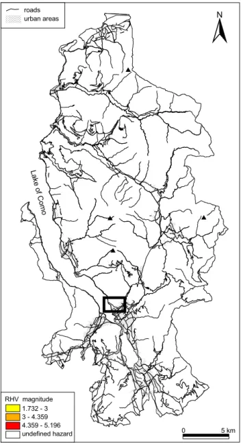
Lake of Como N $ $ # $ $ undefined hazard 4.359 - 5.196 3 - 4.359 1.732 - 3 RHV magnitude urban areas roads 0 5 km

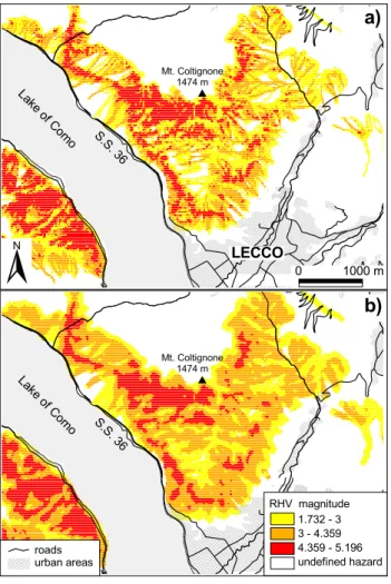
Fig. 5. Regional rockfall hazard map for the Lecco Province

(570 km2). The low resolution of the rockfall model allows for a

preliminary recognition of hazard.

variability of restitution and friction coefficients into speci-fied ranges. Cells exhibiting a very large rockfall count are located mostly along channels or in areas where the topogra-phy concentrates the falling blocks. The maximum computed velocities and heights reach 100 m/s and 500 m, respectively. A map of the translational kinetic energy, to be reclassified for hazard assessment, has been computed by considering a constant block size of 3 m3, corresponding to about 8000 kg, i.e. a representative size for damaging blocks in the area. Model results indicate that 328 342 cells, corresponding to about 131 km2, (23% of the study area), are prone to rock-falls. Figure 4a shows a close-up of the computed rockfall count in the Mt. S. Martino cliff area (northern part of the Lecco urban area). The regional scale model is useful for

large-scale, recognition rockfall analysis and hazard assess-ment, but not suitable for site-specific engineering purposes (Agliardi and Crosta, 2002).

4.2 Local-scale assessment: the Mt. S. Martino-Coltignone area

The Mt. S.-Coltignone area is located north of the city of Lecco and south of the Grigne Massif (Fig. 3). In this area, limestone cliffs up to 400 m high impend directly on some suburbs of Lecco and on the State Road 36, an important transportation corridor connecting the southern Lombardia to Switzerland and Valtellina. The area has been historically prone to rockfalls (e.g. 1931, 2 casualties; 1935; 1950; 1952; 1955, a house destroyed; 1962; 1965; 1969; 1970; 1983, about 4000 m3involved; 1994; 1995; 1996). The most severe event occurred on 22 February 1969 when a 15 000 m3 rock-fall destroyed 2 houses and killed 7 people. After the 1969 rockfall, extensive defensive countermeasures were built, in-cluding several orders of large elastic fences (total length of about 8 km) and a retaining wall 10 m high (Broili, 1973).

A detailed DEM has been specifically prepared for the Mt. S. Martino area at a ground resolution of 5 m by digi-tising and interpolating contour lines at 5 m intervals from a 1:5000 scale raster topographic map. The analysis of large scale multi-temporal aerial stereo-photos (1954, 1962 and 1974 b/w, 1981 color) and ortho-photos (1994 b/w, 2000 color) allowed us to identify the main geomorphological and structural features, the active rocky cliffs and rockfall sources, the land use and vegetation. Field surveys allowed us to validate these data, to collect detailed information for modelling and to assess the geomechanical characteristics of the rock mass. Four joint sets and bedding have been recog-nised, separating blocks ranging in volume between 0.35 m3 and 3.2 m3_{, with an average value of about 1 m}3_{. Plane and}

wedge failure, block toppling and tensile failure proved to be kinematically feasible processes.

A total of 717, 5 × 5 m source cells were identified, corre-sponding to about 0.9% of the study area). As for the regional scale study, the restitution and friction coefficients were ob-tained by merging and reclassifying in a GIS geology, sur-face geology and land use maps, specifically prepared by the authors for this study at the same scale as the topographic data. Table 3 shows the 13 classes in the unique condition map, and the calibrated average values the relevant coeffi-cients. Since detailed geomechanical information was avail-able, the source areas have been subdivided in homogeneous domains with respect to their geomechanical susceptibility to failure. Six major domains have been outlined, depend-ing on the block size (minimum, average, maximum) and the frequency of detachment. This subdivision has been funda-mental to give a hazard zonation in terms of block mass or energy and to include in the analysis the relative susceptibil-ity to rockfalls, a proxy for the onset probabilsusceptibil-ity.

Several simulations have been run using DEMs at differ-ent ground resolutions. The original 5 m DEM has been resampled at 10 m and 20 m, respectively, in order to

eval-undefined hazard 4.359 - 5.196 3 - 4.359 1.732 - 3 RHV magnitude LECCO $ Mt. Coltignone 1474 m S.S. 36 Lake of Como Lake of Como S.S. 36 Mt. Coltignone 1474 m $

a)

b)

Fig. 6. Close-up of the regional scale Lecco Province model (20 m

ground resolution): (a) raw hazard map obtained by the appli-cation of the procedure, classified by the RH V magnitude; (b) “smoothed” hazard map obtained by averaging neighbouring cells through spatial statistics techniques. See text for explanation.

uate the effect of spatial resolution on the resulting hazard maps. Models have been run with a probabilistic approach, by launching a different number of blocks from each homo-geneous source areas. Model calibration has been performed by comparing the results to the extent of talus slopes, the lo-cation of observed blocks, and the runout recorded for the reported historical events (from a few to some hundreds of cubic metres). Different maps of the translational kinetic en-ergy have been computed using fixed block masses for the entire model, namely: 1000 kg, 2700 kg and 8600 kg, corre-sponding to the minimum, average and maximum block size detected in the entire area, respectively. In addition, a set of kinetic energy maps has been calculated using the max-imum, average and minimum block mass value typical of each recognised homogeneous area.

According to the model, the total area exposed to rock-fall hazard amounts to about 33% (681 150 m2) of the model area (2 043 125 m2). Areas exposed to the transit of more than 1 and 5 blocks amount to about the 30% (624 650 m2) and 18% (372 225 m2), respectively. Calibration of the

Table 4. Percentage of elements at risk, belonging to a given

cate-gory, potentially affected by rockfalls in the Lecco Province

element at risk dimension extent damaged

– – %

urban areas [L2] 73 km2 0.7

Roads [L] 667 km 8.5

railway tracks [L] 5 km 10.0

model has been performed through the above mentioned ap-proach. 72% of the mapped large blocks and 67% of the total talus areas are located within sectors affected by com-puted rockfall trajectories. Figure 4b details the local scale model outputs. Rockfall trajectories in vector (point) format are portrayed, showing the high degree of detail of the simu-lation performed at 5 m ground resolution.

4.3 Implementation and evaluation of hazard models The Rockfall Hazard Index/Vector procedure has been ap-plied to the Lecco Province area and the Mt. S. Martino-Coltignone area to obtain different sets of physically-based hazard maps for local end-users and to evaluate their effec-tiveness.

For the Lecco Province area, the results of low resolu-tion modelling have been employed to obtain a prelimi-nary recognition hazard map. Model results provided by STONE in raster format provide a conservative “worst case scenario” of hazard across an area of 570 km2. The final map (Fig. 5) has been classified according to the computed magnitude of the Rockfall Hazard Vector (RH V ) into three classes, namely: 1.732 ≤ |RH V | ≤ 3 (low rockfall hazard), 3 < |RH V | ≤ 4.359 (intermediate rockfall hazard) and 4.359 < |RH V | ≤ 5.196 (high rockfall hazard). A fourth class has been defined representing “undefined hazard” in ar-eas where the rockfalls are not likely to occur according to the results of numerical modelling. It must be noted that, whereas the reclassification of the parameters contributing to hazard is performed according to objective criteria, a unique way to classify the level of hazard portrayed in the final map cannot be identified, since an objective definition of “low”, “moderate” or “high” hazard by means of the RH V mag-nitude doesn’t exist. Thus, the final classification of hazard has been calibrated using available information about docu-mented rockfall events causing fatalities and damage to in-frastructures and lifelines (S. Martino, 1969; Valmadrera, 1981; Onno Lario, 1984; Varenna, 1997, etc.) and geomor-phological data. In addition, hazard classification should be calibrated according to the aim of the hazard assessments (landplaning, regulation or mitigation), the spatial scale of analysis and the frequency and worth of the elements at risk. The hazard map obtained at a regional scale (Fig. 5) is useful to outline the areas more prone to rockfall. These ar-eas are then selected for further local scale analyses taking

N LECCO S. Stefano Como Lake 198 m a.s.l. Rancio Mt. S.Martino 1046 m $ $ Corno Medale 994 m urban area elastic barriers retaining fill rockfall source main roads undefined hazard 4.123 - 5.196 3 - 4.123 1.732 - 3 RHV magnitude a) b) c) d) 0 200 m LECCO S. Stefano Como Lake 198 m a.s.l. Rancio Mt. S.Martino 1046 m $ $ Corno Medale 994 m LECCO S. Stefano Como Lake 198 m a.s.l. Rancio Mt. S.Martino 1046 m $ $ Corno Medale 994 m LECCO S. Stefano Como Lake 198 m a.s.l. Rancio Mt. S.Martino 1046 m $ $ Corno Medale 994 m N N N 0 200 m 0 200 m 0 200 m

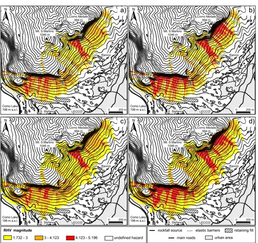
Fig. 7. Hazard maps obtained from the local-scale Mt. S. Martino-Coltignone model (at 5 m resolution). Hazard scenarios obtained by

raster outputs using: (a) mean block mass, (b) maximum block mass. Smoothed maps by averaging RH V values through a 15 m radius neighbourhood analysis for: (c) mean block mass, (d) maximum block mass. Hazard is classified according to the RH V magnitude.

in account the distribution and types of different elements at risk. Due to the scale of analysis, the “raw” hazard map resulting from the application of the assessment procedure (Fig. 5) can be excessively fragmented for practical applica-tions. Thus, spatially distributed statistical techniques have been employed in order to obtain a smoother hazard zona-tion. The “raw” hazard map has been smoothed by averag-ing the RH V magnitude value at each cell with respect to the neighbouring cells within a radius of 20 m. Figure 6 is a close-up of the regional scale hazard model for the area north of Lecco. It clearly shows that the smoothed hazard map is much less fragmented than the “raw” one, resulting in a more effective zonation.

The regional scale hazard model also allows for the pre-liminary evaluation of rockfall risk in the entire Lecco Province, with respect to different involved elements. A rig-orous risk analysis, including the assessment of the vulner-ability, worth and exposure of the elements at risk (Crosta et al., 2001) is beyond the scope of this paper. We simply evaluated the percentage of elements at risk, belonging to a given category, potentially affected by rockfalls, by assuming a unit (maximum) value for exposure. As shown in Table 4, only 0.7% of urbanised areas can be affected by rockfalls, whereas 10% of the roads and 8.5% of the railway tracks are

0.000 0.100 0.200 0.300 0.400 0.500 raw computed

mean RHV (15 m radius neighbourhood) max RHV (15 m radius neighbourhood)

Normalised frequency RHV magnitude range 1.732 - 2.449 _2.449 - 3 3 -3.317 3.317 - 3.464 3.464 - 3.742 3.742 - 4.123 4.123 - 5.196

Fig. 8. Plot of the normalised areal frequency of RH V classes for

different source hazard maps: raw RH V values, smoothed mean and maximum RH V values.

prone to be damage, especially along the main transportation corridor (State Road 36 and the Lecco-Sondrio railway track) to the northern Lombardia. This evaluation is not exhaustive for risk assessment purposes, but provides a first estimate of the most prone elements at risk and their location.

Fig. 9. Example of distributed hazard assessment along linear features: (a) 3-D representation of the hazard map for the Mt. S.

Martino-Coltignone area with the analysed road path, (b) plot of the computed RH V values (smoothed by the mean and the maximum values in the neighbourhood) along the road profile.

rockfall models performed at a ground resolution of 5 m on a small area (about 3 km2) allowed us to obtain hazard maps suitable for planning and mitigation at the Lecco munici-pality scale. Geomechanical characterisation of the involved rock masses (not presented here in detail) allowed us to con-sider different onset probabilities and block masses for each outlined homogeneous domain. By considering the statistical distribution of block masses detected in different areas, dif-ferent hazard maps have been produced, including in the haz-ard assessment kinetic energies corresponding to the mean and maximum block masses.

Also for the Mt. S. Martino-Coltignone area, the hazard maps have been classified according to the computed magni-tude of the Rockfall Hazard Vector (RH V ). In this case, the three hazard classes have been defined as: 1.732 ≤

|_{RH V | ≤ 3 (low hazard), 3 < |RH V | ≤ 4.123}

(inter-mediate hazard) and 4.123 < |RH V | ≤ 5.196 (high haz-ard). Class boundaries have been calibrated in detail using the record of historical events affecting the area in the last four decades. The resulting maps have been smoothed using a similar approach to that used for the regional scale hazard model to produce a more readable, less fragmented hazard map (Figs. 7c and d). Smoothing was done by neighbour-hood analysis within a radius of 15 m.

Smoothing the computed hazard maps through neighbour-hood statistics techniques could eventually lead to unrealis-tic hazard scenarios, i.e. smoothing operations could result in too conservative or optimistic hazard maps, depending on the employed statistics. In Fig. 8, we plot the areal frequency (normalised by the total area prone to rockfalls) of different

RH V values for the “raw” computed hazard map and the

smoothed hazard maps. The smoothing has been performed by computing the mean or maximum values in the neighbour-hood analysis (radius of 15 m). The use of mean values from the neighbourhood analysis results in a more conservative hazard map. Largest deviations of the smoothed RH V val-ues from the raw computed ones occur for the “Flow hazard” cells (Fig. 8), whereas the number of “high hazard” cells

re-mains substantially unchanged. In addition, a redistribution of “high hazard” cells can be observed: areas characterised by high hazard become more continuous, while meaningless isolated “high hazard” pixels disappear. Thus, hazard maps smoothed by the mean RH V values are regarded to be rep-resentative of the computed hazard scenario and suitable as planning tools. On the contrary, hazard maps smoothed by using the maximum RH V in the neighbourhood result in unacceptably high hazard ratings, that are not feasible for practical assessment purposes.

Maps obtained through the proposed procedure can be em-ployed for hazard assessment along linear features (trans-portation corridors, lifelines, etc.). We report an example of rockfall hazard assessment for a road running along the toe of the Mt. S. Martino-Corno Medale slopes (Fig. 9a). The RH V magnitude values have been sampled from the smoothed hazard maps along the the road (Fig. 9a). The val-ues are plotted versus the progressive distance (Fig. 9b), from the lower to the maximum elevation. RH V values sampled every 5 m from previously smoothed hazard maps have been used for the evaluation of the most hazardous sectors along the road. This results could be useful to optimise mainte-nance and remediation works.

The highly detailed analysis at local scale allowed us to evaluate the sensitivity of hazard maps to the input parame-ters, their format (raster/vector) and spatial resolution. This leads to a more objective choice of the “best” hazard map with respect to the quality of the data and to the modelling approach. Different hazard maps has been obtained by using raster modelling outputs and by employing different masses, namely: 1000 kg (fixed for the entire model), and the mean and maximum masses for each of the homogeneous geome-chanical domains (Fig. 7). The same analysis has been per-formed at different spatial resolution, namely: 5 m, 10 m and 20 m, using resampled DEMs (Fig. 10). The resulting hazard maps have been compared by means of diagrams portraying the areal frequency (normalised by the total area prone to rockfalls) of the different RH V magnitude values (Fig. 11).

N b) LECCO S. Stefano Como Lake 198 m a.s.l. Rancio Mt. S.Martino 1046 m $ $ Corno Medale 994 m LECCO S. Stefano Como Lake 198 m a.s.l. Rancio Mt. S.Martino 1046 m $ $ Corno Medale 994 m a) 0 200 m c) LECCO S. Stefano Como Lake 198 m a.s.l. Rancio Mt. S.Martino 1046 m $ $ Corno Medale 994 m 0 200 m RHV magnitude undefined hazard 4.123 - 5.196 3 - 4.123 1.732 - 3 main roads

rockfall source elastic barriers retaining fill urban area

0 200 m 0 200 m

Fig. 10. Comparison of the hazard maps obtained for the Mt. S. Martino-Coltignone area at different spatial resolution (5 m, 10 m and 20 m, respectively). Model raster outputs and a constant block mass have been employed.

We observe that:

– at any spatial resolution (Figs. 11a, b and c), an

in-crease of the block mass results in increasingly haz-ardous maps. This effect is more important when the maximum mass is used. This is obvious, since an

in-crease of the input mass results in inin-creased computed kinetic energy;

– the number of high hazard cells increases (Figs. 11d,

e and f) for decreasing model resolution. This can be related to the higher velocities computed for low reso-lution models, which increase the computed kinetic en-ergy (Agliardi and Crosta, 2002; Agliardi and Crosta, 2003);

– the shift toward higher hazard levels, as block mass

increases, is more relevant for lower resolution mod-els. This results from the combination of two factors contributing to hazard by increasing the kinetic energy, namely: larger mass (input) and higher velocity (com-puted for lower resolutions).

The aforementioned observations stress the importance of collecting accurate geomechanical and topographic data. The frequency distribution of block size for a homogeneous source area is required in order to introduce onset probability and to choose among different modelling approaches. The mean observed mass can be used to represent the most com-mon hazard scenario. The maximum mass can be used if more conservative results are needed when highly populated areas or extremely valuable elements at risk are involved. It is worthwhile to recall that the raster outputs of the program STONE are themselves conservative, since they represent the worst kinematic conditions. Thus, they are suitable for re-gional scale analyses, whereas, at local scales, vector out-puts should be used. In fact, they provide local kinematic information allowing for more accurate hazard assessment (Fig. 12) and for a better compromise between safety and ur-ban development.

5 Concluding remarks

Spatially distributed assessment of rockfall hazard is a diffi-cult, intrinsically uncertain operation. The proposed method-ology is based on the numerical modelling of rockfall trajectories, performed with a spatially distributed, three-dimensional rockfall simulation program (Agliardi et al., 2001; Guzzetti et al., 2002). The Rockfall Hazard In-dex/Vector assessment procedure is mainly focused on the propagation phase of rockfalls, which is responsible of most of the uncertainty affecting the analysis. The onset (or trig-gering) probability is to be independently evaluated prior to the modelling phase, by geomechanical and/or probabilistic analyses, whose discussion is beyond the aim of this pa-per. The onset probability is introduced in the simulations through the number of launched blocks from different source areas, affecting the rockfall occurrence probability at a given location to which simulated rockfalls propagate.

The proposed hazard assessment procedure minimizes subjectivity in the choice of the criteria used to reclassify the involved parameters. We propose the Rockfall Hazard Vector to overcome the ambiguity in hazard ranking allow-ing a direct and objective hazard zonation. If this is accepted,

20m, 1 ton block 20m, mean mass 20m, max mass 5m, max mass 10m, max mass 20m, max mass 5m, 1 ton block 5m, mean mass 5m, max mass 5m, 1 ton block 10m, 1 ton block 20m, 1 ton block 1.5 2 2.5 3 3.5 4 4.5 5 5.5 RHV magnitude Normalised frequency 0.000 0.100 0.200 0.300 0.400 0.500 10m, 1 ton block 10m, mean mass 10m, max mass 5m, mean mass 10m, mean mass 20m, mean mass 1.5 2 2.5 3 3.5 4 4.5 5 5.5 RHV magnitude Normalised frequency 0.000 0.100 0.200 0.300 0.400 0.500 1.5 2 2.5 3 3.5 4 4.5 5 5.5 RHV magnitude Normalised frequency 0.000 0.100 0.200 0.300 0.400 0.500 1.5 2 2.5 3 3.5 4 4.5 5 5.5 RHV magnitude Normalised frequency 0.000 0.100 0.200 0.300 0.400 0.500 1.5 2 2.5 3 3.5 4 4.5 5 5.5 RHV magnitude Normalised frequency 0.000 0.100 0.200 0.300 0.400 0.500 1.5 2 2.5 3 3.5 4 4.5 5 5.5 RHV magnitude Normalised frequency 0.000 0.100 0.200 0.300 0.400 0.500

a)

b)

c)

d)

e)

f)

Fig. 11. Quantitative comparison of the different hazard maps obtained for the Mt. S. Martino-Coltignone area with different combinations

of block mass and spatial resolution. Diagrams portray the areal frequency of the different values of RH V magnitude.

1.5 2 2.5 3 3.5 4 4.5 5 5.5 RHV magnitude Normalised frequency 0.000 0.100 0.200 0.300 0.400 0.500

5m, 1 ton block, vector 5m, 1 ton block, raster

Fig. 12. Comparison between hazard models with same resolution

(5 m) and block mass (1 ton), but employing vector and raster model outputs.

the users only need to concentrate their attention on the con-struction of reliable rockfall numerical models. Neverthe-less, different types of hazard problems (i.e. point-like, lin-ear and areal problems) require different definitions for the occurrence probability and intensity. Thus, different

ver-sions of the method could be implemented and modified to be suitably applied to different problems. To improve the method and to refine existing empirical and semi-empirical approaches, the results obtained by using the method will be compared to existing hazard assessment methodologies (Cancelli and Crosta, 1993; Rouiller and Marro, 1997; Crosta and Locatelli, 1999). Applications of the modelling approach to the planning and design of countermeasures by including hazard values is currently under development.

The method will be further developed to be used in dif-ferent “rockfall settings” and to provide guidelines for the evaluation of hazard map quality to be adopted by regional and local administrations in charge of the public safety and land planning.

Acknowledgements. The authors are grateful to R. Detti for

com-puter programming, and to M. Marian for his invaluable help in the preparation of the DEM of the Mt. S. Martino and in the test-ing of the hazard assessment procedure. F. Guzzetti is thanked for the continuous and clarifying discussions on the hazard assessment techniques. D. Fossati and M. Ceriani are thanked for providing useful criticisms. The research was carried in the framework of the EC DAMOCLES project (UE EVG1-CT-1999-00007 grant).

References

Agliardi, F., and Crosta, G. B.: 3-D numerical modelling of rock-falls in the Lecco urban area (Lombardia Region, Italy), in: Proc. EUROCK 2002, I.S.R.M. International Symposium on Rock En-gineering for Mountainous Regions, Madeira, edited by Dinis de Gama, C. and Ribeiro e Sous, L., Sociedade Portuguesa de Geotecnica, 79–86, 2002.

Agliardi, F. and Crosta, G. B.: High resolution three-dimensional numerical modelling of rock falls, Int. J. Rock Mech. Min. Sci., 40/4, 455–471, 2003.

Agliardi, F., Crosta, G. B., Guzzetti, F., and Marian, M.: Method-ologies for a physically-based rockfall hazard assessment, Geo-physical Research Abstracts, 4, EGS02-A-04594, 2002. Agliardi, F., Cardinali, M., Crosta, G. B., Guzzetti, F., Detti, R., and

Reichenbach, P.: A computer program to evaluate rockfall haz-ard and risk at the regional scale, Examples from the Lombhaz-ardy Region, Geophysical Research abstract, 3, 8617, 2001.

Agostoni, S., Laffi, R., Dell’Orsina, F., Pasotti, J., and Sganga, F.: Carta inventario delle frane e dei dissesti della Provincia di Lecco, Regione Lombardia – Provincia di Lecco – Universit`a degli Studi di Milano, GNDCI publication no. 1942, 182 (in Ital-ian), 1999.

Azzoni, A., La Barbera, G., and Zaninetti, A.: Analysis and predic-tion of rockfalls using a mathematical model, Int. J. Rock Mech. Min. Sci. & Geomech. Abstr., 32 7, 709–724, 1995.

Bozzolo, D. and Pamini, R.: Simulation of rockfalls down a valley site, Acta Mechanica, 63, 113–130, 1986.

Bozzolo, D., Pamini, R., and Hutter, K.: Rockfall analysis – a math-ematical model and its test with field data, Proc. 5th Int. Sympo-sium on Landslides, Lausanne, Switzerland, 1, 555–563, 1988. Broili, L.: In situ tests for the study of rock fall, Geologia Applicata

e Idrogeologia, 8, 1, 105–111 (in Italian), 1973.

Bunce, C. M., Cruden, D. M., and Morgenstern, N. R.: Assessment of the hazard from rockfall on a highway, Can. Geotech. J., 34, 344–356, 1997.

Cancelli, A. and Crosta, G. B.: Hazard and risk assessment in rock-fall prone areas, in: Risk Reliability in Ground Engineering, edited by Skipp B.O., Inst. Civ. Eng., Thomas Telford, 177–190, 1993.

Chau, K. T, Wong, R. H. C., and Wu, J. J.: Coefficient of restitution and rotational motions of rockfall impacts, Int. J. Rock Mech. Min. Sci., 39, 69–77, 2002.

Crosta, G. B. and Locatelli, C.: Approccio alla valutazione del ris-chio da frane per crollo, Proc. Studi geografici e geologici in onore di Severino Belloni, Glauco Brigatti Publisher, Genova, 259–286 (in Italian), 1999.

Crosta, G. B. and Agliardi, F.: Frane di crollo e caduta massi: aspetti geomorfologici, modelli teorici e simulazione numerica, Report EU programme Interreg IIC – Falaises, 119 (in italian), 2000.

Crosta, G. B., Frattini, P., and Sterlacchini, S.: Valutazione e ges-tione del rischio da frana: principi e metodi, Regione Lombardia Publication, Milano, 169 (in Italian), 2001.

Descouedres, F. and Zimmermann, Th.: Three-dimensional dy-namic calculation of rockfalls, Proc. 6th Int. Congress of Rock Mechanics, Montreal, Canada, 337–342, 1987.

Dussauge-Peisser, C., Helmstetter, A., Grasso, J. R., Hantz, D., Desvarreux, P., Jeannin, M., and Giraud, A.: Probabilistic ap-proach to rock fall hazard assessment: potential of historical data analysis, Natural Hazard and Earth System Sciences, 2, 1/2, 15– 26, 2002.

Einstein, H. H.: Special lecture: Landslide risk assessment proce-dure, Proc. 5th Int. Symp. on Landslides, Lausanne, 2, 1075– 1090, 1988.

Evans, S. G. and Hungr, O.: The assessment of rockfall hazard at the base of talus slopes, Can. Geotech. J., 30, 620–636, 1993. Falcetta, J. L.: Un nouveau modle de calcul de trajectoires de

blocs rocheux, Revue Francaise de Geotechnique, 30, 11–17 (in French), 1985.

Fell, R.: Landslide risk assessment and acceptable risk, Can. Geotech. J., 31, 2, 261–272, 1994.

Fell, R. and Hartford, D.: Landslide risk management, in: Landslide risk assessment, edited by: Cruden, D., and Fell, R., Balkema, Rotterdam, 51–109, 1997.

Gerber, W.: Direttiva per l’omologazione delle reti paramassi, Ufficio Federale dell’ambiente, delle foreste e del paesaggio (UFAFP), Istituto federale di ricerca WSL, Berna, 39 (in Italian), 2001.

Guzzetti, F.: Landslide fatalities and the evaluation of landslide risk in Italy. Eng. Geol., 58, 89–107, 2000.

Guzzetti, F., Carrara, A., Cardinali, M., and Reichenbach, P.: Land-slide hazard evaluation: a review of current techniques and their application in a multi-scale study, Central Italy, Geomorphology, 31, 181–216, 1999.

Guzzetti, F., Crosta, G. B., Detti, R., and Agliardi, F.: STONE: a computer program for the three-dimensional simulatation of rock-falls, Computers and Geosciences, 28, 9, 1081–1095, 2002. Hungr, O. and Evans, S. G.: Engineering evaluation of fragmental rockfall hazards. Proceedings 5th International Symposium on Landslides, Lausanne, 1, 685–690, 1988.

Hungr, O., Evans, S. G., and Hazzard J.: Magnitude and frequency of rockfalls and rock slides along the main transportation cor-ridors of south-western British Columbia, Can. Geotech. J., 36, 224–238, 1999.

Interreg IIC: Prevenzione dei fenomeni di instabilit delle pareti roc-ciose. Confronto dei metodi di studio dei crolli nell’arco alpino, Final Report EU Programme Interreg IIC – Falaises, 239 (in French/Italian), 2001.

Jones, C. L., Higgins, J. D., and Andrew, R. D: Colorado Rockfall Simulation Program Version 4.0, Colorado Department of Trans-portation, Colorado Geological Survey, 127, 2000.

Kobayashi, Y., Harp, E. L., and Kagawa, T.: Simulation of rock-falls triggered by earthquakes, Rock Mech. Rock Eng., 23, 1–20, 1990.

Matsuoka, N. and Sakai, H.: Rockfall activity from an alpine cliff during thawing periods, Geomorphology, 28, 309–328, 1999. Mazzoccola, D. and Sciesa, E.: Implementation and comparison

of different methods for rockfall hazard assessment in the Ital-ian Alps, Proc. 8th Int. Symp. On Landslides, Cardiff, Balkema, Rotterdam, 2, 1035–1040, 2000.

Pfeiffer, T. and Bowen, T.: Computer simulation of rockfalls, Bull. Ass. Eng. Geol., 26, 1, 135–146, 1989.

Pierson, L. A., Davis, S. A., and Van Vickle, R.: Rockfall Haz-ard Rating System Implementation Manual, Federal Highway Administration (FHWA), Report FHWA-OR-EG-90-01, FHWA, U.S. Department of Transportation, 1990.

Ritchie, A. M.: Evaluation of rockfall and its control, Highway Re-search Board, Highway Res. Rec., 17, 13–28, 1963.

Rochet, L.: Application des modles num´eriques de

propaga-tion a l’´etude des ´eboulements rocheux, Bulletin Liaison Pont Chauss´ee, 150/151, 84–95 (in French), 1987.

Rouiller, J. D. and Marro, C.: Application de la methodologie Mat-terock a l’evaluation du danger li`e aux falaises, Eclogae Geol.

Helv., 90, 393–399 (in French), 1997.

Scioldo, G.: Rotomap: analisi statistica del rotolamento dei massi. Guida Informatica Ambientale, P`atron, Milano, 81-84 (in Ital-ian), 1991.

Spang, R. M.: Protection against rockfall – stepchild in the design of rock slopes, Proc. 6th Int. Congress on Rock Mechanics, Mon-treal, Canada, 551–557, 1987.

Stevens, W.: RocFall: a tool for probabilistic analysis, design of remedial measures and prediction of rockfalls, M.A.Sc. Thesis, Department of Civil Engineering, University of Toronto, Ontario, Canada, 105, 1998.

Van Dijke, J. J. and Van Westen, C. J.: Rockfall hazard: a geomor-phologic application of neighbourhood analysis with Ilwis, ITC Journal, 1990–1, 40–44, 1990.

Varnes, D. J.: Slope movements: types and processes, in: Landslide analysis and control, edited by: Schuster, R. L., and Krizek, R. J., Transportation Research Board, Special Report 176, Washing-ton, DC, 11–33, 1978.

Varnes, D. J. and IAEG Commission on Landslides and other Mass Movements: Landslide hazard zonation: a review of principles and practice, UNESCO Press, Paris, 63, 1984.

Wieczorek, F. G., Morrissey, M. M., Iovine, G., and Godt, J.: Rock-fall Potential in the Yosemite Valley, California, U.S. Geological Survey Open-File Report 99–578, 10, 1999.

Wu, S. S.: Rockfall evaluation by computer simulation: Transporta-tion Research Record, TransportaTransporta-tion Research Board, Washing-ton, DC, 1031, 1–5, 1985.