HAL Id: insu-02183026
https://hal-insu.archives-ouvertes.fr/insu-02183026
Submitted on 8 Dec 2020
HAL is a multi-disciplinary open access
archive for the deposit and dissemination of sci-entific research documents, whether they are pub-lished or not. The documents may come from teaching and research institutions in France or abroad, or from public or private research centers.
L’archive ouverte pluridisciplinaire HAL, est destinée au dépôt et à la diffusion de documents scientifiques de niveau recherche, publiés ou non, émanant des établissements d’enseignement et de recherche français ou étrangers, des laboratoires publics ou privés.
Improved ozone DIAL retrievals in the upper
troposphere and lower stratosphere using an optimal
estimation method
Ghazal Farhani, Robert J. Sica, Sophie Godin-Beekmann, Gérard Ancellet,
Alexander Haefele
To cite this version:
Ghazal Farhani, Robert J. Sica, Sophie Godin-Beekmann, Gérard Ancellet, Alexander Haefele. Improved ozone DIAL retrievals in the upper troposphere and lower stratosphere using an opti-mal estimation method. Applied optics, Optical Society of America, 2019, 58 (6), pp.1374-1385. �10.1364/AO.58.001374�. �insu-02183026�
Improved ozone DIAL retrievals in the upper
troposphere and lower stratosphere using an optimal
estimation method
GHAZALFARHANI1,*, ROBERTJ. SICA1, SOPHIEGODIN-BEEKMANN2, GÈRARDANCELLET2,AND
ALEXANDERHAEFELE3
1Department of Physics and Astronomy, The University of Western Ontario, 1151 Richmond St., London, ON, N6A 3K7 2Observatoire de Versailles Saint-Quentin-en-Yvelines, Guyancourt, France 78280
3Federal Office of Meteorology and Climatology MeteoSwiss, Payerne, Switzerland 1530 *Corresponding author: [email protected]
Compiled October 31, 2018
We have implemented a first-principle Optimal Estimation Method to retrieve ozone density profiles us-ing simultaneously tropospheric and stratospheric Differential Absorption Lidar (DIAL) measurements. Our retrieval extends from 2.5 km to about 42 km in altitude, and in the upper troposphere and the lower stratosphere (UTLS) it shows a significant improvement in the overlapping region, where the OEM can retrieve a single ozone profile consistent with the measurements from both lidars. Here stratospheric and the tropospheric measurements from the Observatoire de Haute Provence are used, and the OEM retrievals in the UTLS region compared with coincident ozonesonde measurements. The retrieved ozone profile have a small statistical uncertainty in the UTLS region relative to individual determinations of ozone from each lidar, and the maximum statistical uncertainty does not exceed a maximum of 7%. © 2018 Optical Society of America
http://dx.doi.org/10.1364/ao.XX.XXXXXX
1. INTRODUCTION
The upper troposphere and lower stratosphere (UTLS) extends from about 6 km to 25 km in height and plays a significant role in the atmospheric climate system. In this region of the atmosphere, even small changes in temperature and in the distribution and concentration of greenhouse gases can result in large changes in atmospheric radiative forcing, which can trigger climate change [1,2].
Ozone in the upper troposphere acts as the third largest greenhouse gas contributing to the radiative forcing of climate change [1,3]. The ozone distribution in the UTLS is the result of transport mechanisms and photochemical reactions. Because of stratospheric tropospheric exchange, large spatial and temporal variability can be observed in the UTLS [4].
In many studies on the UTLS ozone, satellite-borne instruments are used. In limb-viewing instruments, the elevation angle of the line-of-sight varies during the measurements. As a result, limb sounders can provide good vertical resolution (about 2 km to 4 km). However, at lower altitudes (lower troposphere), the atmosphere becomes nearly opaque, and the limb-viewing instruments have difficulties measuring trace gases. Nadir-viewing instruments can provide measurements in the lower troposphere, but their vertical resolution is limited (about 6 km to 7 km). Occultation instruments use the Sun or other stars as the source of radiation, and they can obtain measurements with higher vertical resolution (about 1 km to 2 km). Solar occultation instruments are restricted by the number of sunsets and sunrises they encounter in one orbit, while
stellar occultation instruments are limited by the weakness of the stellar source compared to the Sun. The combination of measurements from different geometrical-based satellite instruments has been used to measure ozone density.
In the UTLS, large biases (differences) in ozone measurements are reported between instruments. Although the difference between the data sets is more significant in the tropics and high latitudes (about± 30%), significant bias exists at mid-latitudes (about±10%) [5]. Therefore, a continued detailed intercomparison between satellite instruments, as well as between satellites and other instruments, is needed, including both airborne measurements and ground-based measurements.
Differential Absorption Lidar (DIAL) systems provide ozone measurements with high vertical and temporal resolutions. For example, observatories such as the Canadian Network for the Detection of Atmospheric Change (CANDAC) Polar Environment Atmospheric Research Laboratory (PEARL) in Eureka, Maïdo ob-servatory in Reunion Island, the Observatoire de Haute Provence (OHP) in France, and the NASA Table Mountain Observatory (TMO) in the United States are equipped with both tropospheric and stratospheric lidars. At the Eureka observatory, the tropospheric lidar system makes measurements from 0.5 km to about 8 km in altitude and the stratospheric lidar system operates from about 4 km to 35 km [6,7]. At the Maïdo observatory, the tropopspheric DIAL makes measurements from 6 km to 16 km, and the stratospheric DIAL operates in the 13 km to 38 km region [8]. At the OHP observatory, the tropospheric DIAL system operates from 2.5 km to about 14.5 km, and the stratospheric DIAL operates from about 10 km to 45 km [9,10]. At the TMO, the tropospheric DIAL system obtains measurements from 3 km to 18 km, and the stratospheric DIAL system from 10 km to 40 km [11,12]. Although these systems can produce satisfactory ozone profiles in their overlapping region (from tropospheric lidar to stratospheric lidar), the uncertainty of merging is not well defined. Providing a single ozone profile with a full uncertainty budget using both sets of measurements can significantly improve our measurements of ozone in the UTLS [13–15].
Here we apply the Optimal Estimation Method (OEM) to tropospheric and stratospheric DIAL measure-ments. Measurements from these two systems are simultaneously used by the retrieval to obtain a single ozone profile. Using the OEM there is no need to “merge” or “glue” level 0 profiles. Moreover, the input measurements can be in different units with different measurement grids (for example a mix of analog and digital measurements). Additionally, a full uncertainty budget, including both the systematic and statistical uncertainties, is calculated for each individual profile. The OEM also provides averaging kernels of the re-trievals, which allows comparison of the profiles with other measurements which can account for differences in vertical resolution, such as when compared to space-based measurements. Other atmospheric and systematic parameters such as air density, the dead time of the system, and the background counts can be retrieved along with ozone profiles. The application of OEMs to aerosol lidar measurements, Rayleigh scatter temperatures, and Raman scatter water vapour retrievals has been studied and discussed in detail [16–18]. In addition, we have recently demonstrated an OEM for DIAL stratospheric ozone retrievals [19], which we will now expand to include measurements from tropospheric ozone DIAL systems.
In this paper, focusing on the UTLS region, we show a first principle OEM to retrieve a single ozone profile by using both tropospheric and stratospheric DIAL measurements directly from the raw (level 0) measurements using the lidar equation as the forward model. In Section2, pre-processing steps prior to applying the traditional DIAL algorithm, as well as the OEM, are discussed. Moreover, the state vectors and the b parameter quantities are defined and a brief overview of the lidar’s specifications is given. In Section3
results of the OEM retrieval, using both tropospheric and stratospheric lidar measurements, are discussed in detail. In this Section, we also show our results of comparison between the ozonesonde profiles and our retrievals. Section4is the summary of the paper, and in Section5we discuss our future plans. Details of how to apply our method to a standalone tropospheric DIAL are given in the Appendix.
2. METHODOLOGY
In the DIAL system, two wavelengths are simultaneously transmitted to the atmosphere. One of the emitted wavelengths is strongly absorbed by the constituent of interest (called the “on-line” wavelength) and the other is weakly absorbed (called the “off-line” wavelength). For ozone measurements, selecting a wavelength pair
depends on the altitude range of the measurements. For most studies, the ultraviolet (UV) spectrum is the most efficient spectral region. A pair of wavelengths with strong UV absorption is needed to detect the small amount of ozone which resides in the troposphere. However, for stratospheric ozone measurements, choosing a laser that can reach higher altitudes in the stratosphere is the main concern [11,20,21].
The traditional analysis method for ozone number density uses the derivative of the ratio between the “on-line” and “off-line” channels to calculate the ozone number density no3(z). A detailed discussion on the
tropospheric and stratospheric ozone retrievals can be found in [10,22–25]. In the traditional analysis, some corrections are applied to the raw lidar measurements, for example background counts should be removed. In many systems this requires including the effects of signal-induced-noise (SIN). Any corrections due to nonlinearity of the counting system (because of saturation) should also be applied to the raw counts. Finally, the signals from different channels need to be merged to form a single measurement profile. This “corrected” count profile is then used to calculate the ozone number density profiles. With the OEM, a forward model encapsulates the geophysical properties and instrumental characteristics of the system, and our OEM retrieval uses the raw (level 0) measurements from all available channels. A comprehensive explanation of the OEM can be found in [26]; a brief description of the OEM follows below.
In the OEM a forward model is defined as the relation between the measurements vector y = (y1, y2, ..., yn),
and the state vector x = (x1, x2, ..., xn). The forward model is:
y = F(x, b) + e (1)
where b are the forward model parameters, which are assumed to be known, and e is the measurement noise. We use the lidar equation as the forward model, where the raw counts are the measurements. The lidar equation for unsaturated counts, Ntrue, is:
Nobs(z, λi) = C(λi)O(z) z2 β(λi, z) exp[−2 Z ∞ 0 [σO3(λ, T(z))nO3(z) + α(λ, z) +
∑
e σe(λ)ne(z)]dz] + Nb(z, λi) (2)where Nobs(z, λi) is the number of backscattered photons. C(λi) is the lidar constant, which contains the area
of the receiving telescope, the total efficiency of the lidar system, and energy of the scattered photon. The geometrical overlap is O(z), and β(λi, z) are the atmospheric backscattering coefficients which includes both
molecular and aerosol terms. The first term inside the integral corresponds to ozone absorption in which
σO3(T(z), λi) is the ozone absorption cross section, which depends on atmospheric temperature, and nO3(z) is
the ozone number density. The second term of the integral, α(λ, z) contains the extinction coefficient which is the sum of the extinction due to molecules and particles, and the last term∑eσe(λ)ne(z) is the extinction
by other absorbers. For ozone studies, the most common interfering gases are SO2, NO2and O2. The effect
of O2is only considered when the selected “on-line” laser wavelength is shorter than 294 nm [12,27]. In the
case of heavy volcanic eruption, SO2and NO2can significantly affect ozone retrievals [28]. However, in most
cases, for both stratospheric and tropospheric ozone studies the effect of these gases in final ozone retrievals is negligible. Thus, the last term of integration is typically neglected [10].
The background counts are written as Nb(z). In the presence of SIN, the background is fitted to an exponential
function of the form:
Nb(z) = a exp(−bz) + c (3)
where a, b, and c are coefficients of the fit, which in the traditional method are determined analytically, but are retrieved in our OEM retrieval using the analytic values as a priori coefficients [29].
When the intensity of the backscattered signal is high, the counting system can be affected by saturation. This saturation can result in an observed count rate which is less than the true count rate. For a paralyzable detector, true counts are related to the observed counts Nobsas follows:
Nobs = Ntrueexp(−κ Ntrue) (4)
and, for non-paralyzable detectors, the following equation can be used: Nobs =
Ntrue
1 + κNtrue
where κ is the dead time of the detecting system. For the OEM retrieval the value of the dead time for each channel is retrieved.
A. Implementing the OEM for the OHP lidars
Knowing the measurements vector and its covariance matrix Se, and using an a priori profile and its associated
covariance matrix Sa, the OEM calculates an optimal a posteriori state by minimizing a cost function:
Cost = (y−Kx)TS−y1(y−Kx) + (x−bx)TS−a1(x−bx) (6)
As our forward model is nonlinear, an iterative numerical method is used. For our problem the Levenberg-Marquardt iteration is a suitable numerical method. Then, the optimized state vector x is given as:
xi+1= xi+ [(1 + γi)S−a1+ KTi SyKTi]−1([KTi S−y1(y−F(xi, b)]−S−a1(xi−xa)) (7)
where i is the iteration term, xa is the a priori profile, and K = dFdx is the linearisation term for our nonlinear forward model, called the Jacobian matrix. Finally, γiis a damping factor for the iteration, which is chosen at
each step to minimize the cost function. As suggested by [30] if the value of the cost function increases in a step, γiwill increase by a factor of 10, and if the value of the cost function decreases in a step, γi will decrease
by a factor of 2. The iteration stops when the cost function decreases to a value much smaller than the number of measurements. There are other criteria which result in ceasing the iteration. Further details can be found in [26].
To understand how measurements and a priori profiles contribute in the final retrievals, an averaging kernel can be used. The relation between the retrieved state and the true state is described by the averaging kernel of the retrieval. The averaging kernel is calculated as:
A= dbx
dx = [K
TS−1
y K+ S−a1]−1KTS−y1K (8)
The retrieved quantity (bx) can be written as follows: b
x = (I−A)xa+ Ax + er (9)
where eris the retrieval uncertainty and I is a unity matrix. A perfect retrieval, in the sense all the information
comes from the measurement with no effect from the a priori state, has averaging kernels equal to one, where the first term of the above equation becomes zero. The width of the averaging kernel gives the resolution of the retrieval at each height, here defined as the Full Width Half Maximum (FWHM) of each averaging kernel. In order to find the state vector (from Eq.7) the following quantities should be known: the measurements and their covariances, the a priori profiles, the a priori profile’s covariance, and the model (b) parameters. The b parameters are quantities in the forward model that are not being retrieved, because they are either well-known or retrieving them is not possible. The uncertainty associated with the retrieval due to the b parameters is calculated after the last iteration of the solution. The forward model and the Jacobians (K) for each of the state vectors are calculated, and the Qpack package is used to perform the retrieval. Details of the Qpack software are given in [31].
Here we retrieve the ozone density profile, relative air density, dead time values, and background counts. Overlap functions, ozone cross sections, and Rayleigh scattering cross sections are considered as b parameters in the forward model. Below, we discuss our choices of a priori profiles and b parameter values. The covariance matrices associated with the measurements and a priori profiles are discussed as well, and these values are summarized in Table1.
In photon counting mode, when the signal is linear, the measurements statistical uncertainty follows a Poisson distribution, and the number of counts at each altitude represents the measurement’s variance at that height. There is no correlation between the digital counts in different layers of the atmosphere, so the off-diagonal elements of the measurement’s covariance matrix are zero. However, for the OHP lidars, analog measurements do not follow Poisson distributions. Calculating the measurement variance for each
measurement point requires selecting n points before and after the specified point, and then fitting a straight line to these 2n + 1 points, which is then removed. Next, the residual variance is calculated. For our measurements, we tried different values for n, and n = 3 provided the best fit for our measurements.
In order to determine the background counts in both the tropospheric and stratospheric measurements, the mean of the counts above a specific height is calculated and used as the a priori for the “off-line” channels, since SIN is negligible in these channels. The variance of the background counts divided by the number of bins in the selected region is the uncertainty for the background a priori value. For “on-line” channels where SIN is present, an exponential function is fitted to the signal and the coefficients of the fit are used as a priori values. An uncertainty of 20% is assigned to these coefficient a priori values. The altitude above which the background counts are determined is different for tropospheric and stratospheric lidars. Also, as the laser power in the “online” channel is about 2 times stronger than the laser power in the “off-line” channel, the effect of SIN in the “on-line” channel is more pronounced. The values we chose for the OHP lidars measurements are shown in
Table1.
We retrieve the logarithm of ozone density profile. This choice is numerically more favourable to show small changes in large numbers. The U.S standard model is used as the a priori ozone profile [32]. An uncertainty of 20% is assigned to this profile.
We retrieve the air density for both tropospheric and stratospheric measurements. However, below 15 km the air density profile retrieved is in fact a convolution of air density and aerosol load. Mass Spectrometer Incoherent Scatter Radar (MSIS) total density profiles are used as a priori profiles, and an uncertainty of 20% is assigned to it [33]. To generate a full length a priori covariance matrix for both air and ozone density profiles at altitudes below 12 km, a tent function with a correlation length of 300 m was used. At altitudes above 12 km the correlation length was increased to 900 m. This choice of correlation length is because above 12 km, the stratospheric lidar measurements have the most weight and the retrieval grid for these measurements starts at 300 m. Using the forward model, the a priori of the lidar constants for both tropospheric and stratospheric lidars are estimated. We assign a 10% uncertainty to the a priori of the lidar constants to account for changes with time of laser power, atmospheric transmission, and system efficiency.
The overlap function, Rayleigh cross sections, and ozone absorption cross sections are assumed as b parameters. Although these parameters are not being retrieved, the uncertainty associated to them contributes to the final uncertainty budget. The assigned values for the overlap function, Rayleigh cross sections and ozone cross section along with their standard deviations are listed in Table (1).
B. Description of the Lidars
The OHP lidars’ station (44◦N, 6◦E) has made routine measurements of ozone in the free troposphere and stratosphere for the last three decades. The transmitter for the tropospheric system uses the fourth harmonic of a Continuum Nd:YAG laser (266 nm) frequency shifted by Raman Stimulated Scattering in a D2 high pressure cell [34]. The DIAL measurement makes use of the 1st and 2nd Raman Stokes lines at 289 nm (the “on-line” wavelength) and 316 nm (the “off-line” wavelength). Backscattered photons are collected by a Cassegrain telescope which is equipped with a 80 cm mirror. For the spectral separation of the two backscatter signals the collected signal is passed from the telescope to a spectrometer.The signals are detected by a photomultiplier tube (PMT). The system configuration is bi-axial, and the distance between the laser and the telescope axes is 0.5 m. The overlap, O(z), is significant from the surface to about 4 km [35].
The stratospheric lidar system uses an XeCl excimer laser at 308 nm, with a repetition rate of 100 Hz. This laser has an output energy of about 200 mJ for the “on-line” channel, while the “off-line” wavelength at 355 nm is generated by the third harmonic of a continuum Nd:YAG laser with an energy of 50 mJ at 50 Hz. The backscattered signal is collected by four Newtonian telescopes, each with diameter of 0.5 m. The collected signal is sent to a spectrometer which separates the signal into four wavelengths. Two of these correspond to the emitted Rayleigh signals at 308 nm and 353 nm. The other two correspond to the Nitrogen Raman shifted spectrum at 331.8 nm and 386.7 nm, respectively. The Rayleigh signals are separated further into high- and low-gain photomultiplier channels. Hence, in total 6 photocount profile measurements are obtained. Further details on the OHP tropospheric and stratospheric lidars can be found in [9,10,34].
Parameter Value Standard Deviation
Stratospheric lidar measurements measured Poisson statistics
Tropospheric lidar measurements (digital channels)
measured Poisson statistics
Tropospheric lidar measurements (analog channels)
measured 3-point running standard
de-viation Retrieved a priori values
Ozone density U.S standard model 20%
Air density MSIS 20%
Deadtime empirical fitting 20%
Background for stratospheric measure-ments (“off-line”)
mean above 80 km σabove 80 km
Coefficients of SIN for stratospheric mea-surements (“on-line”)
empirical fitting above 80 km 20%
Background for tropospheric measure-ments (“off-line”) digital channel
mean above 20 km σabove 20 km
Background for tropospheric measure-ments (“off-line and “on-line”) analog channel
mean above 12 km σabove 12 km
Coefficients of SIN for tropospheric mea-surements (“on-line”) digital channel
empirical fitting above 12 km 20%
Lidar constants estimate from FM 20%
Forward model parameters
Rayleigh-scatter cross section Nicolet (1984) 0.3%
Ozone absorption cross section BDM (1986) 2%
Overlap function available at Dataset CitationA 10%
Dates 12 July 2017 14 July 2017 26 July 2017
Tropospheric lidar 2049 – 2357 2350 – 0219 2140 – 2237
Stratospheric lidar 2106 – 0142 2151 – 0221 2007 – 0016
Ozone sonde 2153 2348 2133
Table 2. Measurements periods for the tropospheric and stratospheric lidars systems and launch times for
the ozonesondes.
3. OEM OZONE RETRIEVAL IN THE FREE TROPOSPHERE AND STRATOSPHERE
In this section we present the result of combining the two lidar measurements to retrieve a single ozone profile. We choose measurements from 12 July 2017 as this night has both clear skies and coincident measurements from the NDACC-LAVANDE intercomparison campaign. The results for the nights of 14 and 26 July 2017 are presented as well (see Table.2). Our first example retrieval will be from the night of 12 July 2012, where the tropospheric lidar operated from 2049 to 2357, and the stratospheric lidar operated from 2106 to 0142 (all local time). An ozonesonde was launched at 2153 from the OHP station and the tropopause height was at 14.7 km. For the tropospheric lidar system, the native resolution of measurements is 7.5 m for the analog channels and 30 m for the digital channels. For the stratospheric lidar system, the native resolution of measurements for all six channels is 150 m. Our retrieval starts at 2.6 km with a resolution grid of 150 m. At 11 km the retrieval grid changes to 500 m, and at 21 km it changes to 1500 m, and finally, at 25 km height, it becomes 1700 m. We chose these retrieval grids to be closer in vertical resolution to traditional retrieval grids.
The averaging kernels calculated for the retrieval are shown in Fig.1. The shape of the averaging kernels define the sensitivity of the retrieval to the true state. As shown in Eq.9, when the averaging kernel equals 1, the retrieval is sensitive only to the measurements. The vector area of the averaging kernels is defined as
Au, where u is a unity vector. When the area is close to 1, the retrieval is mostly independent of its a priori value. In our retrieval the averaging kernel has an area of about 1 up to 42.2 km, indicating the retrieval is mostly independent of the a priori profile. At about 11 km when the stratospheric measurements are added to the retrieval grids, a small spike is observed in the curve. This spike disappears at higher altitudes.
Fig. 1.Averaging kernels for tropospheric-stratospheric ozone measurements. The averaging kernels are
only shown every 450 m for lower altitude (from 2.5 km to 11 km height), and every 1500 m in higher alti-tudes for clarity. As is shown in the red curve, the area of the averaging kernel matrix has a small spike at 11 km, when the stratospheric ozone measurements are included.
The residual plots, which show the difference between the forward model and the actual measurements, for both the tropospheric and stratospheric lidar are shown in Fig.2. The four plots on top are the residuals for the stratospheric measurements, and the four plots at the bottom are residuals for the tropospheric measurements. As shown in the figure, for both low-altitude and high-altitude channels the forward model can successfully encapsulate the physics of the atmosphere and the characteristics of the lidars, and, up to 50 km, the difference
between the forward model and the actual measurements is less than 5%. The ozone profile for the night
Fig. 2.The percentage difference between the forward model and the actual measurements are shown in
blue. The statistical uncertainty is plotted in red. The four plots on top are the stratospheric forward model residuals, and the four plots at the bottom are the tropospheric forward model residuals. For digital count-ing systems, the Poisson distribution is appropriate and the variance of the measurements at each altitude is the number of photons at that altitude. However, the output signals of the analog channels do not fol-low a Poisson distribution and to find the variance a 3-point running filter is used. As a result the red line (which indicates the noise of measurements) for the analog channels is more structured then for the digital channels.
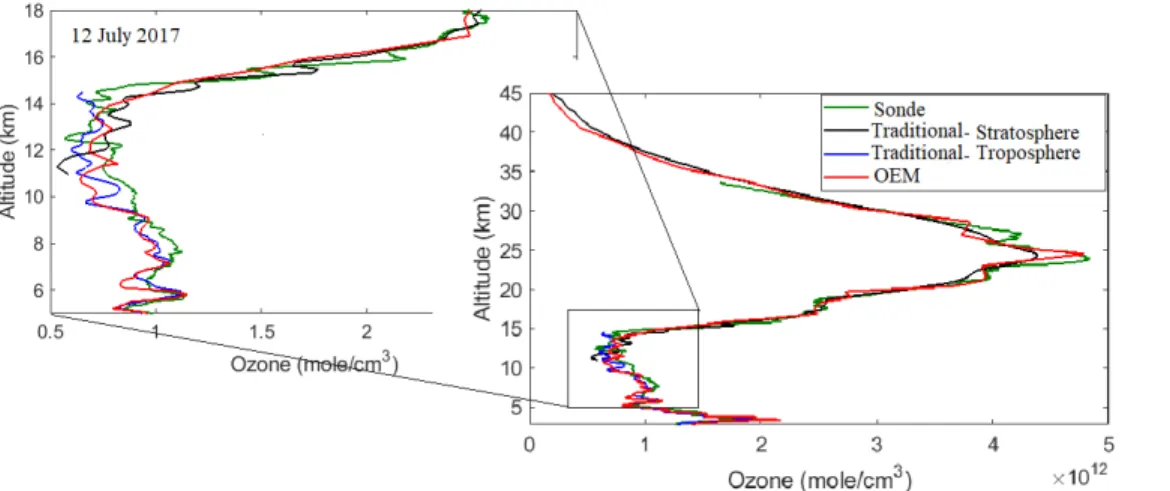
of 12 July 2017 is retrieved from 2.6 km to 42.2 km altitude. In Fig.3the OEM retrieval is plotted against the traditional stratospheric and tropospheric retrievals. The traditional ozone retrieval starts from 2.5 km and extends to 14.5 km, and the traditional stratospheric ozone retrieval starts at 11 km and extends to about 42.2 km. The tropopause height on this night is at 14.7 km. For comparison purposes the ozonesonde profile which starts from the ground and goes up to 33 km is shown as well. On this night of measurements, the ozonesonde balloon was released at 2153 from the station (44◦N, 5.8◦E). During the time of fly it drifted southeastward, such that 1.5 hours later, at the altitude of 33 km, its location was (43.6◦N, 6◦E).
To demonstrate how the OEM retrieval performs in the region where the tropospheric measurements are merged with the stratospheric measurements, we consider the retrievals in the region between 6 km to 17 km. As shown in Fig.3, until about 11 km the OEM retrieval is closer to the traditional tropospheric analysis. At 11 km where the stratospheric measurements are added, the OEM retrieval’s result becomes closer to the traditional stratospheric analysis, though the value of the number density in this region tends to be between the two traditional stratospheric and tropospheric retrieval values.
The vertical resolution of the OEM retrieval is calculated from the full width at half maximum (FWHM) of the averaging kernel at each altitude. The vertical resolutions as well as the statistical uncertainties of the OEM and the traditional retrievals are plotted in Fig.4. In the free troposphere, at an altitude of 2.5 km, the vertical resolution for the OEM retrieval is 150 m, increasing to 300 m at 11 km. The traditional vertical resolution starts at 150 m as well, but grows faster such that at 11 km the vertical resolution is 1000 m (Fig.4, right panel). The trade-off is that the uncertainty of the retrieval in the traditional method is smaller, so that at 11 km it is 4.5% as opposed to the OEM retrieval which has a larger uncertainty of 7.5%. At 11 km where the stratospheric measurements are added, the OEM vertical resolution is 300 m and gradually increases up to 600 m at 14.5 km, whereas, in the traditional tropospheric method, the retrieval resolution increases to 1900 m at the same height. At 21 km altitude, the vertical resolution is 1500 m, while at 25 km it is 1700 m. The vertical resolution does not change until 40 km, where due to the rapid drop in SNR it increases to 2000 m.
The percentage difference between the OEM retrieval and the ozonesonde measurements is shown in Fig.5. For most heights the difference between the OEM retrieval and the sonde measurements in within the uncertainty of the two profiles. At 10 km, the difference between the sonde and the OEM retrieval is almost 30%. Above this altitude, and in the UTLS, the difference between the two profiles is less than 10%
Fig. 3.The OEM retrieval (red curve) compared to the traditional calculation of ozone using the OHP lidar systems. The tropospheric lidar starts at 2.5 km and extends upward to 14.5 km (blue curve). The ozone profile measured by the stratospheric lidar system (black curve) overlaps with the profile retrieved from the tropospheric lidar system in the UTLS. In this region, the OEM retrievals smoothly transition from relying primarily on the tropospheric lidar measurements to the stratospheric measurements.
Fig. 4.Left panel: The statistical uncertainty of the OEM retrieval (red curve) is plotted against the statistical
uncertainty of the traditional retrievals. The uncertainty of the retrieval for the stratospheric and tropo-spheric lidar systems respectively are shown in black and blue. Right panel: The vertical resolution of the OEM retrieval is shown in red. The vertical resolution of the traditional calculation from the tropospheric lidar system is shown in blue, while the vertical resolution of the retrieved profile produced from the strato-spheric lidar system is shown in black.
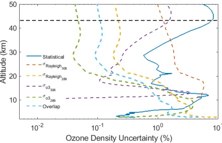
The systematic uncertainties due to Rayleigh cross sections, the ozone absorption cross sections, and the overlap function are the b parameters in the forward model which contribute to the uncertainty of the ozone retrieval. The Rayleigh-scatter cross section uncertainty for both tropospheric and stratospheric lidars has a significant contribution. At lower altitudes (below 5 km) the Rayleigh-scatter uncertainty (for tropospheric lidar measurements) has a value of about 10%. At higher altitudes (above 14 km), this value becomes less than 1%. In the stratosphere, the Rayleigh-scatter uncertainty is about 8% (at 15 km height) and this value drops to about 1% at altitudes above 20 km. These values for the tropospheric and stratospheric Rayleigh-scatter uncertainties agree with the calculated values in the Leblanc et al. NDACC Lidar Working group [36] uncertainty budget for the traditional calculation (respectively 8% and 10%). The ozone absorption cross section for the 289 nm channel is about 5% which is close to the 7% uncertainty calculated by [36]. For stratospheric measurements, the ozone uncertainty has its maximum of 4% at the bottom of retrievals, which is higher than the calculated uncertainty of 2% in [36] uncertainty budget. The uncertainties due to the overlap function at is 5% at the
Fig. 5.The percentage difference between the OEM retrieval and the ozonesonde measurements (blue curve) is plotted within the total statistical uncertainty of the OEM retrievals plus the ozonesonde mea-surement (red curves).
bottom of retrieval and, at 10 km it drops to about 1%. The uncertainty due to the ozone cross sections at 316 nm and 353 nm are negligible and are not shown in this plot. Also, the uncertainty on the retrieved ozone profile due to the temperature uncertainty of the ozone cross section is negligible as well.
Fig. 6.Uncertainty budget on the night of 12 July 2017. The statistical uncertainty of the retrieval (blue), the
Rayleigh-scatter cross section uncertainty at 308 nm (dashed line red), the Rayleigh-scatter cross section un-certainty at 289 nm (dashed line yellow), the ozone absorption cross section at 308 nm (dashed line purple), the ozone absorption cross section for the 289 nm channel (dashed line green), and the overlap function for the 289 nm channel (dashed line light blue) all contribute to the budget. The horizontal dashed line shows the height below which the retrieval is independent of the a priori profile.
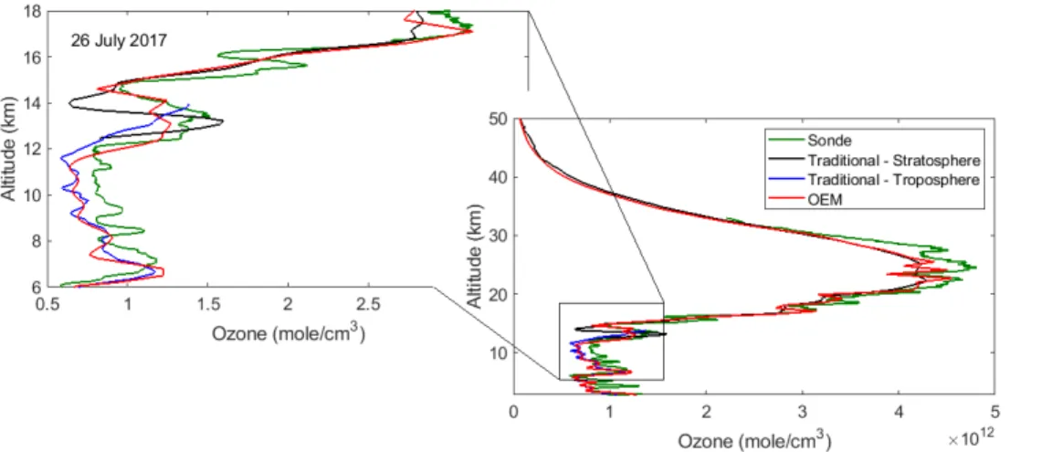
Ozone density profiles are also retrieved for the nights of 14 July 2017, and 26 July 2017, each of which also had coincident ozonesonde measurements. On July 14 2017 the tropopause height is 12.5 km. The traditional retrievals of tropospheric and stratospheric lidars, at altitudes between 10 km to 15 km, are not consistent with each other (Fig.7). The percentage difference between the traditional tropospheric and stratospheric ozone profiles in this region reaches its maximum of 33% at a height of 11.8 km. The OEM retrieval, similar to the night of 12th July, smoothly hands off from one lidar’s measurements to the other one, and in this case is closer to the traditional stratospheric DIAL measurement. Also, the statistical uncertainty of the OEM retrieval reaches its maximum at about 12 km. The figure also shows the OEM retrieval compared with the sonde measurements. The ozonesonde was released from the station (44◦N, 5.8◦E) and it flew to the southeast. At its maximum height, the ozonesonde was located at (43.5◦N, 6.3◦E), and was not more than 50 km away from the
OHP station. Similar to 12 July 2017, the percentage difference between the OEM and the sonde measurements is within the two profiles uncertainty.
On the night of 26 July 2017, the two ozone profiles calculated by the traditional method are inconsistent in the region from 12 km to 14 km are inconsistent with each other in the region of the tropopause (13.3 km). The OEM retrieval can smoothly transition from the tropospheric measurements to the stratospheric measurements (Fig. 8). Although, the OEM and the traditional analysis in the lower troposphere are match well (their difference is about 2%), the sonde profile is far from the two retrievals, and the difference between the sonde measurements and the lidar measurements (both the OEM and the traditional analysis) is greater than 60%. The ozonesonde, similar to the other nights, was released from the station, but comparing to the other nights it moved slightly farther toward the south, such that at its maximum height its location was (43.1◦N, 5.8◦E). Thus, the sonde was within approximately 100 km of its launch point.
Fig. 7.OEM ozone-profile retrieval on 14 July 2017 (red curve). The tropospheric traditional retrieval (blue
curve) extends from 2.5 km to 15 km, while the stratospheric traditional retrieval (black curve) extends from 10 km to 43 km. At the region where the tropospheric and stratospheric lidar measurements overlap, the OEM can smoothly makes a transition from one lidar system’s measurements to the other system’s measurements.
4. SUMMARY
We have introduced a first-principles OEM retrieval for tropospheric ozone profiles, as well as for a combination of tropospheric and stratospheric ozone profiles. Using the DIAL lidar measurements, we retrieved ozone profiles starting in the free troposphere and extending to the upper stratosphere. The results from our implementation of the OEM are summarized below.
1. The forward model uses the lidar equation and works directly with the raw measurements. The forward model provides a robust estimate of ozone profiles for clear nights.
2. The combined stratospheric-tropospheric DIAL OEM retrieval calculate a single ozone profile consistent with all the measurements.
3. A new retrieval method for tropospheric DIAL ozone lidars is given in the Appendix.
4. We used four different channels for tropospheric ozone retrievals, and eight different channels for the stratospheric-tropospheric ozone retrievals. The OEM has the advantage of using all these measurements at the raw (level 0) stage; thus, no gluing or merging of profiles is needed.
Fig. 8.OEM ozone-profile retrieval on 14 July 2017 (red curve). The tropospheric traditional retrieval (blue curve) extends from 2.5 km to 14 km, while the stratospheric traditional retrieval (black curve) extends from 12.5 km to 43 km. At the region where the tropospheric and stratospheric lidar measurements overlap, the OEM can smoothly makes a transition from one lidar system’s measurements to the other system’s measurements.
6. In the UTLS, the OEM retrieval smoothly transitions from one lidar system to the other system. The vertical resolution of the OEM retrievals in this region is about 600 m, and the retrieval uncertainty due to measurement noise does not exceed 7%.
7. Both tropospheric and tropospheric-stratospheric retrievals provide a full uncertainty budget which includes both statistical and systematic uncertainties.
5. CONCLUSIONS
We used simultaneous tropospheric and stratospheric lidar measurements with the OEM to retrieved ozone profile from 2.5 km to above 40 km. The OEM method has no need for “gluing” or “merging” the tropospheric and stratospheric measurements, as all measurements are simultaneously considered when retrieving a single ozone profile. Therefore, unlike the traditional method in which the two profiles can show considerable differences in the UTLS, our OEM retrieval provides a single ozone profile consistent from the measurements from both lidar systems, and includes the vertical resolution and a complete uncertainty budget. This result is a significant advantage of the OEM.
Our forward model has been tested under clear sky conditions. However, in the UTLS region, clouds and significant aerosol loads can exist. We are planning to augment our forward model to allow for inclusion of aerosols, as well as other trace gases. Furthermore, as our methods allows the calculation of averaging kernels for the retrieval, we are interested in comparing our retrievals with satellite measurements, as well as processing more of the OHP measurements.
6. APPENDIX 1: TROPOSPHERIC OZONE LIDAR RETRIEVALS
We have demonstrated a retrieval for stratospheric ozone profiles using the OEM and measurements from a stratospheric DIAL lidar [19]. In addition to the combined retrieval discussed here, the OEM retrieval presented in this work can be applied separately to tropospheric lidar systems. For tropospheric DIAL lidars, the overlap function must be added to the forward model, and this is the main difference between the two systems aside from including the different parameters associated with the different choice of wavelengths in a tropospheric DIAL system. Another difference is that for the OHP tropospheric lidar, the analog channel counts (as discussed in details inA) do not follow a Poisson distribution.
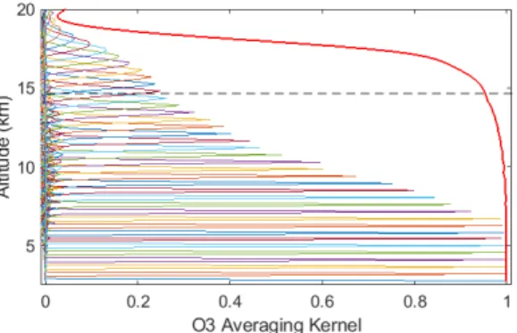
The averaging kernels for the tropospheric retrieval is shown in Fig.9. Below 14.2 km (where the horizontal dashed line is plotted), at least 90% of the ozone profile is retrieved from the measurements. Although, the retrieval extends to 16.5 km, we only consider the retrieved profile up to 14.2 km in height (above this altitude, the ozone profile starts falling into the a priori profile). In higher altitudes when the SNR drops, the averaging kernel becomes smaller and the retrieval falls back to its a priori value. The residual plots are similar to one shown in Fig.2.
Fig. 9.Averaging kernels for the ozone density for the measurements on 12 July 2017. The horizontal
dashed line is the height cut-off above which the sensitivity of the retrieval to measurements is less than 90%. The averaging kernels are only shown every 450 m in altitude. The summation of rows in the averag-ing kernel matrix, for each specific height, is shown by the red curve.
The retrieval starts from 2.5 km, with 150 m steps, and extends to 14.2 km. The ozone retrieval resulting from the OEM code is plotted against the sonde profile and the traditional profiles (see Fig.10). The OEM retrieval and the traditional method are within good agreement for most heights. Above 12 km the difference between the OEM and the traditional profile reaches to its maximum of 25%.
Fig. 10.Both the OEM retrieval (red curve) and the traditional retrieval (blue curve) extend from 2.5 km to
14.2 km. The ozonesonde profile is plotted in green. The black dashed line defines the cut-off altitude of the retrieval.
The statistical uncertainties and vertical resolution of the traditional and OEM retrievals are shown in Fig.11. The OEM retrieval has a better vertical resolution but higher uncertainty. The OEM retrieval resolution at 2.5 km is 150 m and at 14.2 km it becomes 600 m. As shown in the right panel of Fig.11, the vertical resolution in the OEM retrieval is 200 m until about 10 km altitude. At an altitude of 5.5 km, where the photon counting signals are added, a small spike is observed. The traditional vertical resolution starts at 150 m and reaches to 1500 m at 14.2 km. The uncertainty of the OEM and the traditional method are similar for the first few kilometers. At 5.5 km, where the digital measurements begin, both methods have an uncertainty smaller than 1%. Above 5.5 km, the uncertainty in the OEM retrieval grows larger, and at 14.2 km it becomes 10.2%. The
uncertainty of the traditional retrieval becomes larger as well, however at 14.2 km it is 7%. As shown in our stratospheric retrieval, the data and retrieval grids, as well as the correlation lengths, in the OEM method can be chosen to trade off larger vertical resolution for lower statistical uncertainty, like in the traditional method.
Fig. 11.Left panel: The statistical uncertainty of the OEM retrieval (red curve) as well as the statistical
uncer-tainty of the traditional retrieval (blue curve) for 12 July 2017. Right panel: Vertical resolution of the OEM retrieval is shown in red, while the vertical resolution of the traditional retrieval is shown in blue. The spike at 5.5 km in the OEM uncertainty is from the inclusion of the digital channels at this height.
OEM tropospheric ozone profile have also been retrieved for measurements on the nights of 14 July 2017 and 26 July 2017. The OEM retrieval for the night of 14th July is in good agreement with the traditional method, and for most heights, the difference between the two methods is small. At 11.5 km, the OEM retrieval has a better agreement with the sonde profile, but the difference between the two methods is only 2.5%, which is within their statistical uncertainty (see Fig.12). On 26 July, at all altitudes above 3 km, the difference between the traditional and the OEM retrievals is less than 2%.
Fig. 12.For the nights of 14 July and 26 July 2017, the tropospheric OEM retrieval is shown in red, the
tradi-tional retrieval is in blue, and the ozonesonde profile is in green. The horizontal dashed line is the “cut-off” altitude below which the OEM retrieval is mostly independent of the a priori ozone profile assumed. Left panel: retrievals for 14 July 2017. Right panel: retrievals for 26 July 2017.
A. Dataset Citation
G. Ancellet, ftp://ftp.cpc.ncep.noaa.gov/ndacc/meta/lidar/ga-ohp-tropo-ldr.txt FUNDING
This project has been funded in part by the National Science and Engineering Research Council of Canada. The OHP system is funded by The National Center for Scientific Research.
ACKNOWLEDGEMENTS
We would like to thank Shayamila Mahagammulla Gamage for interesting discussions and help. We also appreciate Patricia Sica’s patience and help with the editing of this paper. We would like to thank the lidar operators of the station Gèrard Mègie at Haute-Provence Observatory. Ghazal Farhani also would like to thank friends at LATMOS and MeteoSwiss for their hospitality.
REFERENCES
1. IPCP, “Climate change 2007: The physical science basis,” Agenda6, 333 (2007).
2. J. A. Logan, “Tropospheric ozone: Seasonal behavior, trends, and anthropogenic influence,” J. Geophys. Res. Atmospheres90, 10463–10482 (1985).
3. V. Ramaswamy, O. Boucher, J. Haigh, D. Hauglustine, J. Haywood, G. Myhre, T. Nakajima, G. Y. Shi, and S. Solomon, “Radiative forcing of climate,” Clim. change349 (2001).
4. F. Forster, M. Piers, and K. P. Shine, “Radiative forcing and temperature trends from stratospheric ozone changes,” J. Geophys. Res. Atmospheres102,
10841–10855 (1997).
5. M. I. Hegglin and H. Tegtmeier, “The sparc data initiative: Assessment of stratospheric trace gas and aerosol climatologies from satellite limb sounders,” SPARC Rep. (2017).
6. J. Seabrook and J. Whiteway, “Influence of mountains on arctic tropospheric ozone,” J. Geophys. Res.: Atmospheres121, 1935–1942 (2016).
7. A. B. Tikhomirov, G. Farhani, E. McCullough, R. J. Sica, T. Leblanc, and J. R. Drummond, “Ozone measurements using the refurbished eureka stratospheric dial,” Can J Remote. Sens. (submitted).
8. J. L. Baray, Y. Courcoux, P. Keckhut, T. Portafaix, P. Tulet, J. P. Cammas, A. Hauchecorne, S. Godin Beekmann, M. D. Mazière, C. Hermans et al., “Maïdo observatory: a new high-altitude station facility at reunion island (21° s, 55° e) for long-term atmospheric remote sensing and in situ measurements,” amt6, 2865–2877 (2013).
9. A. Gaudel, G. Ancellet, and S. Godin-Beekmann, “Analysis of 20 years of tropospheric ozone vertical profiles by lidar and ecc at observatoire de haute provence (ohp) at 44° n, 6.7° e,” Atmospheric Environ.113, 78–89 (2015).
10. S. Godin-Beekmann, J. Porteneuve, and A. Garnier, “Systematic dial lidar monitoring of the stratospheric ozone vertical distribution at observatoire de haute-provence (43.92[degree]n, 5.71[degree]e),” J. Environ. Monit.5, 57–67 (2003).
11. G. J. Megie, G. Ancellet, and J. Pelon, “Lidar measurements of ozone vertical profiles,” Appl. Opt24, 3454–3463 (1985).
12. M. F. Mérienne, A. Jenouvrier, B. Coquart, M. Carleer, S. Fally, R. Colin, A. C. Vandaele, and C. Hermans, “Improved data set for the herzberg band systems of 16o 2,” J. Mol. Spectrosc.207, 120–120 (2001).
13. J. R. Holton, P. H. Haynes, M. E. McIntyre, A. R. Douglass, R. B. Rood, and L. Pfister, “Stratosphere-troposphere exchange,” Rev. Geophys.33, 403–439
(1995).
14. A. Stohl, P. Bonasoni, P. Cristofanelli, W. Collins, J. Feichter, A. Frank, C. Forster, E. Gerasopoulos, H. Gäggeler, P. James et al., “Stratosphere-troposphere exchange: A review, and what we have learned from staccato,” J. Geophys. Res.: Atmospheres108 (2003).
15. Y. Cohen, H. Petetin, V. Thouret, V. Marécal, B. Josse, H. Clark, B. Sauvage, A. Fontaine, G. Athier, R. Blot et al., “Climatology and long-term evolution of ozone and carbon monoxide in the upper troposphere–lower stratosphere (utls) at northern midlatitudes, as seen by iagos from 1995 to 2013,” acp
18, 5415–5453 (2018).
16. A. C. Povey, R. G. Grainger, D. M. Peters, and J. L. Agnew, “Retrieval of aerosol backscatter, extinction, and lidar ratio from raman lidar with optimal estimation,” amt7, 757–776 (2014).
17. R. J. Sica and A. Haefele, “Retrieval of temperature from a multiple-channel rayleigh-scatter lidar using an optimal estimation method,” Appl. Opt54,
1872–1889 (2015).
18. R. J. Sica and A. Haefele, “Retrieval of water vapor mixing ratio from a multiple channel raman-scatter lidar using an optimal estimation method,” Appl. Opt55, 763–777 (2016).
19. G. Farhani, R. J. Sica, S. Godin-Beekmann, and A. Haefele, “Optimal estimation method retrievals of stratospheric ozone profiles from a dial lidar,” AMTD2018, 1–22 (2018).
20. E. V. Browell, “Differential absorption lidar sensing of ozone,” IEEE77, 419–432 (1989).
21. A. Papayannis, G. Ancellet, J. Pelon, and G. Megie, “Multiwavelength lidar for ozone measurements in the troposphere and the lower stratosphere,” Appl. Opt29, 467–476 (1990).
22. G. Ancellet, A. Papayannis, J. Pelon, and G. Megie, “Dial tropospheric ozone measurement using a nd: Yag laser and the raman shifting technique,” JTECH6, 832–839 (1989).
23. S. Godin, A. I. Carswell, D. P. Donovan, H. Claude, W. Steinbrecht, I. S. McDermid, T. J. McGee, M. R. Gross, H. Nakane, P. J. Daan, Swart, B. B. Bergwerff, O. Uchino, P. von der Gathen, and R. Neuber, “Ozone differential absorption lidar algorithm intercomparison,” Appl. Opt.38, 6225–6236
(1999).
24. I. S. McDermid, S. M. Godin, and D. Walsh, “Lidar measurements of stratospheric ozone and intercomparisons and validation,” Appl. Opt.29, 4914–4923
(1990).
25. T. Leblanc, R. J. Sica, J. A. E. van Gijsel, S. Godin-Beekmann, A. Haefele, T. Trickl, G. Payen, and G. Gabarrot, “Proposed standardized definitions for vertical resolution and uncertainty in the ndacc lidar ozone and temperature algorithms – part 1: Vertical resolution,” amt9, 4029–4049 (2016).
26. C. D. Rodgers, Inverse methods for atmospheric sounding: theory and practice, vol. 2 (World scientific, 2000).
27. S. Fally, A. C. Vandaele, M. Carleer, C. Hermans, A. Jenouvrier, M. F. Mérienne, B. Coquart, and R. Colin, “Fourier transform spectroscopy of the o2 herzberg bands. iii. absorption cross sections of the collision-induced bands and of the herzberg continuum,” J. Mol. Spectrosc.204, 10–20 (2000).
28. D. F. Heath, B. M. Schlesinger, and H. Park, “Spectral change in the ultraviolet absorption and scattering properties of the atmosphere associated with the eruption of el chichón: Stratospheric so2 budget and decay,” Eos Trans. AGU64, 197 (1983).
29. W. H. Hunt and S. K. Poultney, “Testing the linearity of response of gated photomultipliers in wide dynamic range laser radar systems,” IEEE Trans. Nucl. Sci22, 116–120 (1975).
30. R. Fletcher, Practical methods of optimization (John Wiley & Sons, 2013).
31. P. Eriksson, C. Jimenez, and S. Buehler, “Qpack, a general tool for instrument simulation and retrieval work,” J. Quant. Spectrosc. Radiat. Transf.91,
32. A. J. Krueger and R. A. Minzner, “A mid-latitude ozone model for the 1976 us standard atmosphere,” J. Geophys. Res. Atmospheres81, 4477–4481
(1976).
33. A. E. Hedin, “Extension of the msis thermosphere model into the middle and lower atmosphere,” J. Geophys. Res.: Space Phys.96, 1159–1172 (1991).
34. G. Ancellet and M. Beekmann, “Evidence for changes in the ozone concentrations in the free troposphere over southern france from 1976 to 1995,” Atmos. Env.31, 2835–2851 (1997).
35. T. Halldorsson and J. Langerholc, “Geometrical form factors for the lidar function,” Appl. Opt.17, 240–244 (1978).
36. T. Leblanc, R. J. Sica, J. A. E. van Gijsel, S. Godin-Beekmann, A. Haefele, T. Trickl, G. Payen, and G. Liberti, “Proposed standardized definitions for vertical resolution and uncertainty in the ndacc lidar ozone and temperature algorithms – part 2: Ozone dial uncertainty budget,” amt 9, 4051–4078