HAL Id: insu-02937916
https://hal-insu.archives-ouvertes.fr/insu-02937916
Submitted on 17 Nov 2020HAL is a multi-disciplinary open access archive for the deposit and dissemination of sci-entific research documents, whether they are pub-lished or not. The documents may come from teaching and research institutions in France or abroad, or from public or private research centers.
L’archive ouverte pluridisciplinaire HAL, est destinée au dépôt et à la diffusion de documents scientifiques de niveau recherche, publiés ou non, émanant des établissements d’enseignement et de recherche français ou étrangers, des laboratoires publics ou privés.
Electron Temperature in the Pristine Solar Wind: First
Results from the Parker Solar Probe and Comparison
with Helios
M. Maksimovic, S. Bale, L. Berčič, J. Bonnell, A. Case, Thierry Dudok de
Wit, K. Goetz, J. Halekas, P. Harvey, K. Issautier, et al.
To cite this version:
M. Maksimovic, S. Bale, L. Berčič, J. Bonnell, A. Case, et al.. Anticorrelation between the Bulk Speed and the Electron Temperature in the Pristine Solar Wind: First Results from the Parker Solar Probe and Comparison with Helios. Astrophysical Journal Supplement, American Astronomical Society, 2020, 246 (2), pp.62. �10.3847/1538-4365/ab61fc�. �insu-02937916�
Anti-correlation Between the Bulk Speed and the Electron Temperature in the Pristine Solar Wind : First Results from Parker Solar Probe and Comparison with Helios
M. Maksimovic,1 S. D. Bale,2, 3, 4, 5 L. Berˇciˇc,1, 6 J. W. Bonnell,3 A. W. Case,7
T. Dudok de Wit,8 K. Goetz,9 J. S. Halekas,10 P. R. Harvey,3 K. Issautier,1
J. C. Kasper,11, 12 K. E. Korreck,12 V. Krishna Jagarlamudi,8, 1 N. Lahmiti,1 D. E. Larson ,3 A. Lecacheux,1 R. Livi,3 R. J. MacDowall,13 D. M. Malaspina,14 M. M. Martinovi´c,15, 16, 1
N. Meyer-Vernet,1 M. Moncuquet,1 M. Pulupa,3 C. Salem,3 M. L. Stevens,12 ˇ
S. ˇStver´ak,17, 18 M. Velli,19 and P. L. Whittlesey3
1LESIA, Observatoire de Paris, Universit´e PSL, CNRS, Sorbonne Universit´e, Universit´e de Paris, 5 place Jules
Janssen, 92195 Meudon,France
2Physics Department, University of California, Berkeley, CA 94720-7300, USA 3Space Sciences Laboratory, University of California, Berkeley, CA 94720-7450, USA
4The Blackett Laboratory, Imperial College London, London, SW7 2AZ, UK
5School of Physics and Astronomy, Queen Mary University of London, London E1 4NS, UK
6Physics and Astronomy Department, University of Florence, Via Giovanni Sansone 1, I-50019 Sesto Fiorentino, Italy 7Smithsonian Astrophysical Observatory, Cambridge, MA 02138, USA
8LPC2E, CNRS and University of Orl´eans, Orl´eans, France
9School of Physics and Astronomy, University of Minnesota, Minneapolis, MN 55455, USA 10Department of Physics and Astronomy, University of Iowa, IA 52242, USA
11Climate and Space Sciences and Engineering, University of Michigan, Ann Arbor, MI 48109, USA 12Smithsonian Astrophysical Observatory, Cambridge, MA 02138 USA
13Solar System Exploration Division, NASA/Goddard Space Flight Center, Greenbelt, MD, 20771, USA 14Laboratory for Atmospheric and Space Physics, University of Colorado, Boulder, CO 80303, USA
Corresponding author: Milan Maksimovic
15Lunar and Planetary Laboratory, University of Arizona, Tucson, AZ 85719, USA 16Department of Astronomy, Faculty of Mathematics, University of Belgrade, Serbia 17Astronomical Institute, Czech Academy of Sciences, CZ-14100 Prague, Czech Republic 18Institute of Atmospheric Physics, Czech Academy of Sciences, CZ-14100 Prague, Czech Republic 19Department of Earth, Planetary Space Sciences, University of California, Los Angeles CA 90095, USA
(Received September XX, 2019; Revised YY ZZ, 2019; Accepted UU TT, 2019)
Submitted to ApJ
ABSTRACT
We discuss the solar wind electron temperatures Te as measured in the nascent
so-lar wind by Parker Soso-lar Probe during its first perihelion pass. The measurements have been obtained by fitting the high frequency part of Quasi-Thermal Noise spectra recorded on-board by the Radio Frequency Spectrometer (Pulupa et al. 2017). In addi-tion we compare these measurements with those obtained by the electrostatic analyzer
Halekas & al.(2019). These first electron observations show an anti-correlation between Te and the wind bulk speed V : this anti-correlation is most likely the remnant of the
well-known mapping observed at 1 AU and beyond between the fast wind and its coro-nal hole sources, where electrons are observed to be cooler than in the quiet corona. We also revisit HELIOS electron temperature measurements and show, for the first time, that an in-situ (Te, V ) anti-correlation is well observed at 0.3 AU but disappears as
the wind expands, evolves and mixes with different electron temperature gradients for different wind speeds.
Keywords: Solar Wind
1. INTRODUCTION
In thermally driven solar wind models, for which the coronal thermal energy is converted into kinetic solar wind bulk energy, the final asymptotic speed is a function of the initial coronal temperature
(Parker 1958). The hotter the corona, the faster the wind. While this property seems to be verified from remote sensing spectroscopic observations of the corona for minor ions and hydrogen, it does not appear to be correct for the electrons.
Although measuring the coronal proton temperature by means of ultraviolet coronograph spec-trometers is a complex task, it seems well established now that the fast solar wind originates from coronal holes where the hydrogen kinetic temperatures are possibly as large as 4 to 6 million K (Kohl et al. 1996;Cranmer 2002). In addition, the direct correlation between proton temperature and wind speed seems to persist throughout the heliosphere as the well known correlation between the in-situ proton temperature Tp and the bulk speed V , amply described in the literature (Lopez & Freeman 1986; Arya & Freeman 1991; Totten et al. 1995; Matthaeus et al. 2006), and references therein.
As far as electrons are concerned, their temperature in coronal holes is observed to be lower than in the quiet corona (David et al. 1998; Wilhelm et al. 1998; Doschek et al. 2001; Cranmer 2002). In addition the so-called freezing-in temperature of solar wind minor ions, a proxy for the electron temperature at the coronal source obtained from in-situ heliospheric measurements of different heavy ion charge states, exhibits a clear anti-correlation with the local solar wind bulk speed V (Geiss et al. 1995; Ko et al. 1997; Gloeckler et al. 2003; von Steiger & Zurbuchen 2011). This latter anti-correlation has also been inferred by Marsch et al. (1989) who used HELIOS electron data. These authors extrapolated back to the Sun the electron temperature using power law variations of the latter as a function of the solar wind speed.
In this paper we present observations of the solar wind electron temperatures Te measured by the
Parker Solar Probe (PSP) (Fox et al. 2016) during its first perihelion pass in what we may consider to be a nascent, or pristine, solar wind. These measurements have been obtained by using the Quasi-Thermal Noise spectroscopy technique on the one hand and the spacecraft electrostatic analyzer on the other. The measurements reveal a solar wind in the region around 35 solar radii exhibiting a clear and direct anti-correlation between Te and V , as also reported in the companion paper by Halekas & al.(2019). Building on this finding, we revisit HELIOS electron temperature measurements taken at 0.29 AU and beyond, using an analysis technique similar to the one of Marsch et al. (1989). We
show, for the first time directly, that the (Te, V ) anti-correlation is well established also at 0.3 AU but
is cleared gradually as the wind expands (and mixes) with different electron temperature gradients for different wind speeds.
In section2 we describe measurements of the solar wind electrons on PSP. We detail how electron temperatures are retrieved from the high frequency part of the Quasi-Thermal Noise spectra obtained by the electric field antennae. In section3we first describe the published HELIOS data sets which we proceed to re-analyse. Finally in section4we discuss the implications of our results for the dynamical processes underlying solar wind acceleration and evolution.
2. PARKER SOLAR PROBE ELECTRON TEMPERATURE MEASUREMENTS
The solar wind electron velocity distribution functions (VDFs), observed at distances of 0.29 AU from the Sun and beyond, systematically exhibit three different recognizable components: a thermal core and a suprathermal halo, always present at all pitch angles, and a sharply magnetic field aligned strahl that usually moves in the antisunward direction (Feldman et al. 1975;Rosenbauer et al. 1977;
Pilipp et al. 1987; Maksimovic et al. 1997). Whereas the effects of Coulomb collisions may explain the relative isotropy of the core population, the origin of the halo and core populations and their interplay during the wind expansion is currently strongly debated (Maksimovic et al. 2005; ˇStver´ak et al. 2009; Berˇciˇc et al. 2019; Horaites et al. 2019). Are the electron VDFs already non-thermal in the corona as proposed by Scudder (1992a,b) or does this characteristic arise from the expansion of a weakly collisional Maxwellian atmosphere ? One of the key science objectives, among others, of measuring the properties of solar wind electrons with Parker Solar Probe is to understand the origin and evolution of the electron distribution functions and their dynamical role in solar wind acceleration.
In this paper we use data from both the FIELDS (Bale et al. 2016)) and the Solar Wind Electrons Alphas and Protons (SWEAP) (Kasper et al. 2016) instruments on PSP. Solar wind electrons may be diagnosed accurately, both by analyzing the Quasi-Thermal Noise (QTN) spectra (Meyer-Vernet et al. 2017), recorded by the RFS low-frequency receiver (Pulupa et al. 2017) using the FIELDS electric antennas (Bale et al. 2016), or by direct detection of their VDFs with the Solar Probe
Analyzer (SPAN) on-board SWEAP (Whittlesey & al. 2019). In the next subsection we detail the way in which the total electron temperature may be retrieved from the high frequency part of the RFS spectra using QTN analysis, and in the subsequent one we present some of the early SWEAP electron measurements, that will be shown to be broadly consistent with those obtained via QTN.
2.1. Quasi-Thermal Noise measurements using the high frequency part of the RFS spectra
When immersed in a space plasma, an antenna will measure the electrostatic fluctuations induced by the quasi-thermal motion of the ambient electric charges which surround it. The theory of antenna-plasma coupling in space environments out of thermal equilibrium and its use for actual measurements is now well established (Meyer-Vernet 1979;Meyer-Vernet & Perche 1989;Meyer-Vernet et al. 2017). The so-called QTN spectroscopy has been applied successfully to several past missions operating in the solar wind such as ISSE 3 (Meyer-Vernet 1979;Couturier et al. 1981), Ulysses (Maksimovic et al. 1995;Issautier et al. 1999), WIND (Maksimovic et al. 1998) or STEREO (Martinovi´c et al. 2016). It has been implemented on the FIELDS instrument to provide accurate measurements of the electron density and temperature of the outer corona down to 10 Solar radii (Bale et al. 2016).
The first results of the QTN measurements on PSP are described in detail in the current issue by (Moncuquet & al. 2019). These authors present a method which yield the total electron density Ne, the core temperature Tc and a suprathermal temperature. Note that in this study, this latter
suprathermal temperature is actually the total contribution of the halo + strahl thermal pressure. As a complementary method, we use, in the present paper, the high frequency part of the QTN spectra recorded by RFS, above the plasma peak. For this frequency range, the contributions of the proton Doppler-shifted thermal noise and the electron shot noise, including the current-biasing of the antennas which is performed for DC electric fields measurements, are negligible (Meyer-Vernet et al. 2017). Moreover our QTN analysis is mostly dependent on the electron total thermal pressure. Indeed for frequencies f satisfying f fpLD/L where fp and LD are the local plasma frequency
and Debye length respectively, and L the physical length of one arm of the dipole, the QTN is proportional to NeTe/f3 (Meyer-Vernet & Perche 1989).
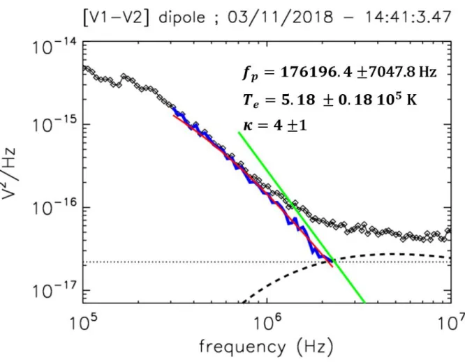
Figure 1. Example of a power spectrum density RFS spectrum measured between 100 kHz and 10 MHz by the FIELDS |V 1 − V 2| antenna dipole (back diamonds). The dotted horizontal line represents the RFS pre-deployment internal noise of ∼ 2.2 10−17V2/Hz. The black dashed line represent the radio galaxy model. The blue and red lines represent the data and the model respectively, which our used for the QTN fitting method described in the text. The green straight line represents an f−3 variation which the QTN spectrum should follow for f fpLD/L.
Another important contribution which need to be taken in our analysis and which can be clearly observed by the RFS radio receiver is the galactic radio background (Cane 1979; Novaco & Brown 1978). This background radiation is relatively constant and covers a 4π solid angle roughly isotrop-ically. Note that modulations of the galactic background as a function of the observed solid angle are less than 20% in the frequency range of consideration (Manning & Dulk 2001). . To obtain the
pure QTN spectrum at high frequency, we have to substract properly the radio galactic background to the total signal.
Figure1 displays a typical power spectral density (PSD) RFS spectrum between 100 kHz and 10 MHz of the FIELDS |V 1 − V 2| antenna dipole. These observations, represented by black diamonds, have been obtained by merging the RFS/HFR and RFS/LFR spectra in one. We did the same for all the data of the first perihelion used here. The dotted horizontal line represents the RFS pre-deployment internal noise which is Vnoise2 ∼ 2.2 10−17V2/Hz in the considered frequency range
(Pulupa & al. 2019). The black dashed line on Figure1represent the RFS PSD Vgalaxy2 corresponding to the (Novaco & Brown 1978) radio galaxy model which we have computed using the detailed method described by (Zaslavsky et al. 2011). More precisely we have used an RFS spectrum measured when PSP was close to 1 AU. At this distance the plasma peak (around 20 kHz) is much lower than the typical fp for the current study. The corresponding QTN spectrum is therefore negligible in the 1 to
10 MHz range at 1 AU. Then taking the observed value of the RFS PSD in the range 2 to 3 MHz and subtracting the above defined receiver noise one obtains a value of ∼ 2.3 10−17V2/Hz for the galaxy PSD in this frequency range. Finally using the (Novaco & Brown 1978) model which yields a radio brightness of 1.1 10−20W/m2/Hz/sr for the corresponding range and applying formula (13) fromZaslavsky et al. (2011) we obtain a reduced effective length of ΓLef f = 1.17 which we can then
use for computing V2
galaxy(f ) on Figure 1.
We can now fit the RFS QTN spectra using the following procedure for each individual RFS |V 1 − V 2| spectrum. We first select all the data frequency points verifying V2
obs(f ) > 3 × Vnoise2 in
the frequency range 300 kHz to 20 MHz. The 300 kHz lower frequency limit has been chosen to be well above fp so that, as described previously, the proton QTN and the shot noise can be neglected.
Then we remove the receiver noise and the galaxy spectrum in order to define the observed QTN spectra V2
obs−QT N(f ) = Vobs2 (f ) − Vnoise2 − Vgalaxy2 (f ) to which we can apply the QTN spectroscopy.
The blue curve on Figure 1 represents V2
obs−QT N(f ) for the considered spectrum. In this particular
case V2
obs−QT N(f ) is only visible up to 2.3 MHz. Above this frequency, it is lower than the sum of the
receiver noise and the galaxy spectrum and thus cannot be measured. The displayed V2
Figure 2. Parker Solar Probe electron temperatures Te,QT N (in black) & 1.47 × Tc,SP AN (in blue), for 12 days around the date of the first perihelion. The solar wind bulk speed V is displayed in red. An anti-correlation between V and both Tc,SP AN and Te,QT N is clearly visible across the time interval.
spectrum is defined on 38 frequency points. The spectra we fit in this study are defined on a number of frequency points which is usually comprised between ∼10 and ∼50 and are never defined on frequencies over 3.5 MHz, because of the galactic background. The final step now consists in fitting V2
obs−QT N(f ) using a full and comprehensive QTN model with Lorentzian VDFs for the electrons
(Chateau & Meyer-Vernet 1989; Zouganelis 2008; Le Chat et al. 2011). This kind of model is well adapted for the high frequency part of the spectra, which is mostly sensitive to the total electron thermal pressure and less to the precise shape of the model VDFs. The red curve on Figure 1
represents the theoretical Lorentzian QTN spectrum which fits the best V2
obs−QT N. Note that for
our fitting procedure we only have two free parameters which are the total temperature Te and the
(2011)). The plasma frequency for each fitted spectrum is set to be the one obtained by the peak tracking method used by Moncuquet & al. (2019) with an uncertainty of 4 %, which is the standard frequency resolution of the RFS. As for Te and the index κ, the uncertainties indicated on the Figure
correspond to the resolution of the model grid which was used for our fitting. Finally the green straight line on Figure1represents an f−3variation which compares well to V2
obs−QT N(f > 1.5MHz).
The QTN temperatures Te,QT N are represented as the black line on Figure 2 for 12 days around
the date of the first perihelion. Te,QT N is ranging between 3 and 6 105 K in good agreement with
an extrapolation of typical 1 AU electron temperatures in the range 1 to 2 105 K and with a typical radial gradient of Te ∝ R−(0.6−0.8) observed in the inner heliosphere (Maksimovic et al. 2000). Note
that we have displayed on Figure 2 only 50% of the data for which the fittings yield a χ2 which is
lower than the median of all χ2.
2.2. SPAN electron measurements
The SPAN instrument is composed of two electron sensors on the ram and anti-ram faces of the spacecraft. They together measure the majority of the three-dimensional electron velocity distribu-tion funcdistribu-tion as explained in detail by Whittlesey & al. (2019). First SPAN observations obtained during the first two PSP perihelia show that there is a large strahl/halo density ratio at 35 Rs
(Halekas & al. 2019). This is in good agreement with the expectations from (Maksimovic et al. 2005;
ˇ
Stver´ak et al. 2009).
In this paper we are using data provided by (Halekas & al. 2019), who have developed a robust fitting procedure to retrieve the electron core temperature Tc,SP AN. This temperature is displayed on
Figure2as the blue line. In order to provide a better visual comparison between Te,QT N and Tc,SP AN
we have multiplied arbitrarily the latter by 1.47 which is the median value of Te,QT N/Tc,SP AN in
the considered time interval. This factor measures actually the contribution of the suprathermal population (halo and strahl) to the electron thermal pressure. Overall the agreement between Te,QT N
and Tc,SP AN is quite good. The linear Pearson correlation between the two datasets is equal to 0.57
for the whole time interval of Figure 2. One should note however that there is a discrepancy between the two temperature during a time interval ranging between 2 and 4 days after the perihelion which
occurred on 2018/11/06 at 03:27. The reason for this discrepancy is still under investigation and is outside the scope of the present paper.
On Figure 2 we have also displayed the solar wind bulk speed V , in red, as measured by the SWEAP Faraday cup instrument (Kasper et al. 2016). A clear anti-correlation between V and both Tc,SP AN and Te,QT N is visible across the time interval. This anti-correlation, which is more pronounced
between V and Tc,SP AN (linear Pearson correlation of -0.59) than between V and Te,QT N (correlation
of -0.20), despite the good correlation between the two temperatures, has also been reported by
Halekas & al.(2019). We now explore this property by re-visiting the Helios data.
3. HELIOS OBSERVATIONS REVISITED 3.1. Helios data sets
In this paper we use three different data sets from the ions and electron electrostatic analyzers on-board the Helios 1 and 2 spacecraft (Schwenn et al. 1975), which performed in-ecliptic measure-ments in the heliocentric distance range between 0.3 and 1 au. The first data set contains ∼1877000 measurements of proton density Np, temperature Tp and bulk speed V measurements. This
con-stitutes the original Helios plasma data set available at ftp://cdaweb.gsfc.nasa.gov/pub/data/helios/ helios1/merged/.
The second and third data sets contain electron density Ne and temperature Te measurements
obtained by fitting the velocity distributions recorded by the I2 electron analyzer (Rosenbauer et al. 1977;Pilipp et al. 1987). This analyzer was designed to measure only 2D distribution functions with an aperture pointing in the ecliptic plane.
The second data set we use has been obtained by ˇStver´ak et al. (2009). These authors used only those measurements for which the magnetic field vector is close enough to the ecliptic plane, that is when Bz/|B| < 0.1. This way they restricted their analysis to the good measurements of the VDFs
in the (v⊥, vk) plane, where the directions ⊥ and k are with respect to the local magnetic field vector.
Finally the last data set we used in this work is obtained in a similar way to that of (ˇStver´ak et al. 2009), but using a slightly different model to describe the velocity distribution of electrons. Details of the data processing can be found in section 3.2 of (Berˇciˇc et al. 2019). This last data set is not limited to the times when the magnetic field lies within the 2D field of view of the electron instrument and therefore only provides good estimations of the perpendicular part of the electron temperature. On the positive hand it gives a better statistics with approximately three times as many point as the (ˇStver´ak et al. 2009) data set.
3.2. Analysis
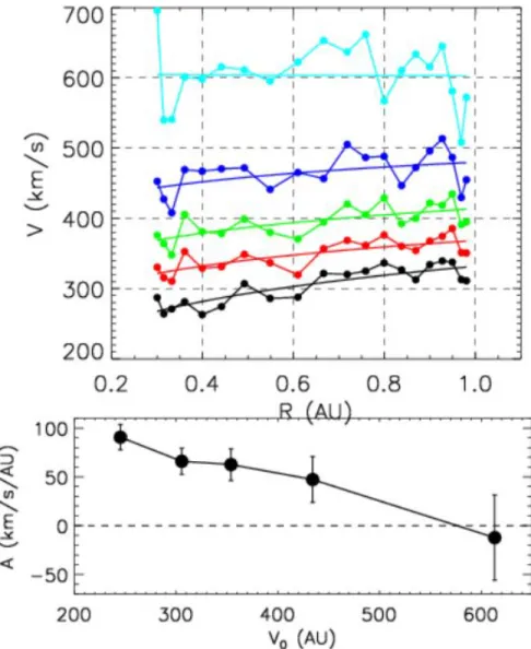
If one displays, for the full Helios data set, the solar wind bulk speed as a function of the heliocentric distance one can note that, while the fastest solar wind flows are bounded by a constant value of about 800 km/s, the slowest solar wind streams increase with radial distance between 0.3 and 1 AU. In order to quantify properly this actual acceleration of the slow solar wind we use a procedure illustrated by Figure 3. We first split the data into 20 heliocentric distance bins. For a statistically representative radial coverage, we define these radial bins so that they each contain an equal number of data points, which is 1877000/20 ∼ 93800. In each of the radial bins we compute the median value of the heliocentric distance and assign it to the radial bin. We then make the assumption that the lowest quintile of the speed data distribution in the first radial bin at ∼ 0.3 AU (black histogram bins on Figure 3) contains the same solar wind streams as the lowest quintile of the data in the following radial bin and so on until the last one at ∼ 0.98 AU. We proceed the same way for the second quintile of the bulk speeds and so on. In such a manner we separate the solar wind into five wind-families which we display using five color codes (black, red, green, blue and cyan in the order of increasing speed values) throughout the paper. For each of these families we compute the median bulk speeds of the five quintiles in each of the 20 radial bins. This leads to 20 (Ri, Vi) data points
which we display on the upper panel of Figure4. We proceed the same way with the protons density (Ri, Npi) and total temperature (Ri, Tpi) data.
On the upper panel of Figure 4 it can be clearly seen that while the bulk speed of the fastest solar wind (cyan) is approximately constant, the bulk speed for the slowest wind (black) is clearly
Figure 3. Illustration of the way we define our wind-families (see text for more details).
increasing. In order to quantify this apparent increase, we have performed a linear fit in the form V (R) = A×RAU+V0 for each of the five wind-families. The lower panel of Figure4displays variation
of the parameters A as a function of V0. This V0 fitting parameter is used in the following in order to
identify the wind-families. Except for the fastest wind (V0 ≈ 600 km/s), all the wind-families with
V0 < 500 km/s exhibit an increase with radial distance which is more important as V0 decreases.
The slowest wind-family (black dots on the upper panel of Figure 4) with a V0 ≈ 250 km/s exhibit
an increase of speed up to ≈ 90 km/s per AU.
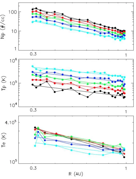
On Figure 5 we display from top to bottom the proton densities (Ri, Npi), proton temperatures
(Ri, Tpi) and the electron temperatures (Ri, Tei) from the (Stver´ˇ ak et al. 2009) data set for the five
wind-families. Note that since there are less data points in the electron data set than in the proton one, we have defined 10 radial bins for the latter case instead of 20. The well known correlations between the proton bulk speed, density and temperature can clearly be seen on Figure5. The fastest is the solar wind (cyan dots), the largest is its proton temperature and the less dens this wind is. In
Figure 4. Upper panel : Median solar wind bulk speeds as a function of the heliocentric distance for the five wind-families. Lower panel: variation of the parameters A as a function of V0 from the linear fit V (R) = A × RAU + V0 for each of the five wind-families.
order to better visualize these correlations, we fit the wind-families proton temperatures with power laws in the form Tp = Tp0× R
αp
AU. The resulting fits are displayed on Figure 5 by full lines of the
same colors as for the wind-families. We do the same for the electron temperatures.
We display the outputs of the above power law fittings on Figure6. One au temperatures Tp0 and
Te0 (upper panel) and power law indexes αp and αe (lower panel) are displayed as a function of V0
Figure 5. From top to bottom: proton density, proton temperature and electron temperature as a function of the radial distance, measured by HELIOS. Color lines show the binned data for our wind families (see text for more explanation).
the major results of this article. While the proton temperature gradients are very similar for the five families with a average power index of ≈ −0.9, this is not the case for the electron gradients. Indeed the temperature gradients for the electrons are quite different, with a clear tendency for the slow wind electron to cool down more steeply (αe ≈ −0.8) than the fast wind ones (αe ≈ −0.3).
Figure 6. Outcome of the power law modelling in the form T = T0× RαAU : One AU temperatures Tp0 and Te0 (upper panel) and power law indexes αp and αe (lower panel) are displayed as a function of V0 for the protons (in red) and the electrons (in black) respectively (see text for more explanation). While the proton temperature gradients are very similar for the five wind speed families, with a average power index of ≈ −0.9, this is not the case for the electrons which exhibit a clear tendency for the slow wind to cool down more steeply (αe≈ −0.8) than the fast one (αe≈ −0.3).
This result is consistent with those obtained by ˚Stver´ak et al. (2015) who show that for the slow wind the electron temperature power law radial dependence is Te ∝ r−0.59 while it is Te ∝ r−0.31
for the fast wind. It is also consistent with the outcome of the study by Marsch et al. (1989) who applied a slightly different technique for binning the data with respect to the bulk speed. Marsch et al. (1989) used actually the same interval limits for the speed bins at all radial distances. This
Protons Electrons Electrons (ˇStver´ak et al. 2009) (Berˇciˇc et al. 2019)
0.29 < RAU < 0.31 0.55 -0.70 -0.94
0.55 < RAU < 0.69 0.72 -0.50 -0.81
0.95 < RAU < 0.98 0.75 0.31 -0.32
Table 1. Linear Pearson correlation coefficients for (Tp, V ) and (Te, V ) for three different radial distances
technique, although similar to ours, does not account for the acceleration of the solar wind, especially for the slowest one. The red triangles connected by a dashed line on the lower panel of Figure 6
represent the αe power law index as a function of V from (Marsch et al. 1989). Note also that the
proton temperature power law indexes we obtain are very similar to those retrieved by Totten et al.
(1995) who used the same technique asMarsch et al. (1989) for binning the data by bulk speed. The black triangles connected by a dashed line on the lower panel of Figure 6 represent the αp power
law index as a function of V from (Totten et al. 1995). Concerning now the values of Tp0 and Te0,
which are the proton and electron modelled temperatures at 1 AU, we retrieve the well known and established correlation between the proton temperature and the wind bulk speed and the lack of such a correlation for the electrons.
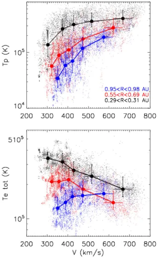
We now explore how these correlations evolve with radial distance. First we down-sample the proton data set to times when the electron measurements in the (ˇStver´ak et al. 2009) data set were performed. We thus present correlations on the same statistical basis for protons and electrons. As done for the latter previously, we now compute the median values (Vi, Tpi) on 10 radial bins Ri
instead of 20. The upper panel of Figure7 displays the proton temperature as a function of the bulk speed for all the points (light dots) and the medians (thick dots) for the first (black), the sixth (red) and the tenth (blue) radial bins. These three radials bins correspond to the following heliocentric distance ranges respectively: 0.29 < RAU < 0.31, 0.55 < RAU < 0.69, 0.95 < RAU < 0.98. Because
the Tp gradients are similar for all the wind-families the 1 AU (V, Tp) correlation is maintained at
all radial distance. This is true both for the medians and for all the data points within a radial bin. This can be seen quantitatively in Table 1, where we have reported the linear Pearson correlation
coefficients between V and Tp for the three radial bins data defined above. While the correlation
coefficient between the proton temperature and speed is equal to 0.75 close to 1 AU, it falls down to 0.55 close to 0.3 AU, but still remains.
For the electrons the tendency is opposite, as one can see on the lower panel of Figure 7. There is a strong (V, Te) anti-correlation at 0.3, with a correlation coefficient of -0.70. This property is most
likely the remnant of the coronal electron temperature mapping. However, as the Te gradients are
quiet different for the different wind-families, the pristine (V, Te) anti-correlation is cleared as the
wind expands. At 1 AU the anti-correlation has completely disappeared on the HELIOS data, with actually a very low (V, Te) correlation coefficient of 0.31. The same trend is also observed using the
(Berˇciˇc et al. 2019) data set, for which we have computed the correlations between V and Te⊥, the
total electron temperature in the perpendicular direction to the magnetic field.
Finally on Figure 8 we have combined the HELIOS electron median temperatures displayed on Figure 7 with those measured by PSP and discussed in section 2. For PSP we have only selected data in the radial range 35.7RS < R < 45RS and binned them on quartiles according to their bulk
speeds. Te,QT N is displayed in magenta while 1.47 × Tc,SP AN is displayed in orange. On can notice
that the limit of the slow wind observed by HELIOS at 66 Rs is shifted to even slower wind speed at 35 Rs, illustrating once more the strong wind acceleration which occurs for the slow wind streams. Another very interesting curve is displayed in green on Figure8. It corresponds to the measurements of the total electron temperatures obtained with the 3DP electrostatic analyser on-board the WIND spacecraft (Lin et al. 1995). For this curve we have accumulated four years of WIND data (1995-1998) and displayed the medians of Te for 8 bins of bulk speed V . The WIND Te variations as a function of
V superimpose almost perfectly with those of HELIOS at 1 AU in the range 350 < V < 600 km/s. Above 600 km/s the WIND Te is anti-correlated with V demonstrating that for these highest speeds
the pristine electron temperature versus bulk speed anti-correlation is conserved up to one AU. As the final conclusion of our analysis, we show Figure 8 that this tendency of different electron thermal gradients for different speed regimes is also valid at the radial distances covered by the Ulysses probe. For this purpose we have used the electron moments of the Ulysses electron analyzer (Bame
Figure 7. Upper panel: proton temperature as a function of the bulk speed for all the points (light dots) and the medians (thick dots) for the first (black), the sixth (red) and the tenth (blue) radial bins. These three radials bins are indicated on the Figure. Lower: same as above for the electrons.
Figure 8. Combined PSP, HELIOS and WIND electron temperature variations as a function of the bulk speed. For PSP Te,QT N is displayed in magenta while 1.47 × Tc,SP AN is displayed in orange. The black, red and blue curves are the HELIOS medians already displayed on Figure7. The green curve corresponds to the medians of the total electron temperatures obtained with the 3DP electrostatic analyser onboard the WIND spacecraft (Lin et al. 1995). The black triangles represent the Ulysses (Vi, Tei) medians for the radial range 1.42 < AU < 1.95, the black squares for 3.01 < AU < 3.54 and the crosses for 4.60 < AU < 5.13. Finally the diamonds represent Ulysses (Vi, Tei) medians for the high latitude regions (see text for more details).
et al. 1992). We have restricted our analysis to the period comprised between the launch in Oct. 1990 and the end of the first orbit on Feb. 1998. We have first divided these data into in-ecliptic, with an absolute value of the spacecraft heliolatitude λ smaller than 20◦, and high latitude, with |λ| > 50◦, regions. The high latitude data correspond to the well known period, during Solar minimum, when
Ulysses was immersed into a very fast wind emanating from polar coronal holes (McComas et al. 2003). The in-ecliptic electron data are represented by the black triangles, squares and crosses on Figure 8, while the high latitude ones are represented by the diamonds. For the in-ecliptic electron data we have applied the same binning technique by speeds and radial distances as previously. The black triangles on Figure 8 represent the (Vi, Tei) medians for the radial range 1.42 < AU < 1.95,
the black squares for 3.01 < AU < 3.54 and finally the crosses for 4.60 < AU < 5.13. It is striking to see on this figure how the primordial anti-correlation in the near solar corona turns into a rough global correlation between V and Te very far from the Sun. As for the high latitude data, the radial
distance covered is comprised between 1.5 and 3.7 AU. When applying our binning technique for these data, and even with different numbers of radial bins, we observe that the (Vi, Tei) medians are
all superimposed to each other. We have thus defined four velocity bins for all the high latitude electron data, independently of the radial distance, and displayed them on Figure 8 with diamonds. As one can see, and contrary to the Ulysses in-ecliptic data, V and Te are anti-correlated when the
bulk speed is large, even far from the Sun.
4. CONCLUSIONS
In this paper we have discussed the first measurements of electron temperatures from Parker Solar Probe over its first orbit with particular emphasis on the first perihelion pass. We have shown that measurements obtained independently using the QTN techniques from the FIELDS experiment are in broad agreement with the direct distribution function results from SPAN on SWEAP. These results show that the nascent, young solar wind observed around 0.15 AU displays a strong anti-correlation of wind speed with electron temperature, in agreement with freezing-in temperature results previously obtained by Ulysses and ACE (Geiss et al. 1995;Gloeckler et al. 1998). In addition, the new analysis of the electron temperatures with both Helios, WIND and Ulysses presented here shows how the in-situ anti-correlation disappears with increasing distance from the Sun, as the solar wind continues to accelerate moving outwards and perhaps also begin to mix. More specifically, the radial electron temperature gradients measured with Helios are found to be very different depending on the solar wind speed, with electron temperatures in the slow wind cooling much faster with distance from
the Sun than electrons in faster winds. The end result is that the electron temperature wind-speed anti-correlation measured in situ by PSP and Helios is lost with increasing radial distances from the Sun. This result provides challenging questions, related to the heating and cooling mechanisms for electrons occurring in different solar wind stream types, and the possible role of evolving in-situ dynamics. While it is well agreed that the amplitude of turbulent fluctuations, especially in faster wind speeds, is sufficient to provide the required heating of protons and ions in the solar wind, for the electrons the interplay of heating, cooling, and thermal conduction, via electromagnetic field fluctuations, instabilities and dynamical evolution of the different parts of the distribution function, and coulomb collisions for the slower parts of the distribution function is more complex and there is no clear relationship between turbulence and heating. So the questions of why the solar wind is born with an anti-correlation between speed and electron temperature, and why the temperature gradients are so different for different solar wind streams are in need of urgent theoretical exploration.
Acknowledgments
Parker Solar Probe was designed, built, and is now operated by the Johns Hopkins Applied Physics Laboratory as part of NASAs Living with a Star (LWS) program (contract NNN06AA01C). Support from the LWS management and technical team has played a critical role in the success of the Parker Solar Probe mission. The FIELDS experiment on the Parker Solar Probe spacecraft was designed and developed under NASA contract NNN06AA01C. The first author wish to thank CNES & CNRS for their support.
REFERENCES
Arya, S., & Freeman, J. W. 1991, J. Geophys. Res., 96, 14183
Bale, S. D., Goetz, K., Harvey, P. R., et al. 2016, SSRv, 204, 49
Bame, S. J., McComas, D. J., Barraclough, B. L., et al. 1992, A&AS, 92, 237
Berˇciˇc, L., Maksimovi´c, , M., Land i, S., & Matteini, L. 2019, MNRAS, 486, 3404 Cane, H. V. 1979, MNRAS, 189, 465 Chateau, Y. F., & Meyer-Vernet, N. 1989,
J. Geophys. Res., 94, 15407 —. 1991, J. Geophys. Res., 96, 5825
Couturier, P., Hoang, S., Meyer-Vernet, N., & Steinberg, J. L. 1981, J. Geophys. Res., 86, 11127
Cranmer, S. R. 2002, SSRv, 101, 229
David, C., Gabriel, A. H., Bely-Dubau, F., et al. 1998, A&A, 336, L90
Doschek, G. A., Feldman, U., Laming, J. M., Sch¨uhle, U., & Wilhelm, K. 2001, ApJ, 546, 559 Feldman, W. C., Asbridge, J. R., Bame, S. J.,
Montgomery, M. D., & Gary, S. P. 1975, J. Geophys. Res., 80, 4181
Fox, N. J., Velli, M. C., Bale, S. D., et al. 2016, SSRv, 204, 7
Geiss, J., Gloeckler, G., von Steiger, R., et al. 1995, Science, 268, 1033
Gloeckler, G., Zurbuchen, T. H., & Geiss, J. 2003, Journal of Geophysical Research (Space
Physics), 108, 1158
Gloeckler, G., Cain, J., Ipavich, F. M., et al. 1998, SSRv, 86, 497
Halekas, J., & al. 2019, in prep. in this issue Horaites, K., Boldyrev, S., & Medvedev, M. V.
2019, MNRAS, 484, 2474
Issautier, K., Meyer-Vernet, N., Moncuquet, M., Hoang, S., & McComas, D. J. 1999,
J. Geophys. Res., 104, 6691
Kasper, J. C., Abiad, R., Austin, G., et al. 2016, SSRv, 204, 131
Ko, Y.-K., Fisk, L. A., Geiss, J., Gloeckler, G., & Guhathakurta, M. 1997, SoPh, 171, 345
Kohl, J. L., Strachan, L., & Gardner, L. D. 1996, ApJL, 465, L141
Le Chat, G., Issautier, K., Meyer-Vernet, N., & Hoang, S. 2011, SoPh, 271, 141
Lin, R. P., Anderson, K. A., Ashford, S., et al. 1995, SSRv, 71, 125
Lopez, R. E., & Freeman, J. W. 1986, J. Geophys. Res., 91, 1701
Maksimovic, M., Bougeret, J. L., Perche, C., et al. 1998, Geophys. Res. Lett., 25, 1265
Maksimovic, M., Gary, S. P., & Skoug, R. M. 2000, J. Geophys. Res., 105, 18337
Maksimovic, M., Hoang, S., Meyer-Vernet, N., et al. 1995, J. Geophys. Res., 100, 19881 Maksimovic, M., Pierrard, V., & Riley, P. 1997,
Geophys. Res. Lett., 24, 1151
Maksimovic, M., Zouganelis, I., Chaufray, J. Y., et al. 2005, Journal of Geophysical Research (Space Physics), 110, A09104
Manning, R., & Dulk, G. A. 2001, Astronomy and Astrophysics, 372, 663
Marsch, E., Pilipp, W. G., Thieme, K. M., & Rosenbauer, H. 1989, J. Geophys. Res., 94, 6893 Martinovi´c, M. M., Zaslavsky, A., Maksimovi´c,
M., et al. 2016, Journal of Geophysical Research (Space Physics), 121, 129
Matthaeus, W. H., Elliott, H. A., & McComas, D. J. 2006, Journal of Geophysical Research (Space Physics), 111, A10103
McComas, D. J., Elliott, H. A., Schwadron, N. A., et al. 2003, Geophys. Res. Lett., 30, 1517 Meyer-Vernet, N. 1979, J. Geophys. Res., 84, 5373
Meyer-Vernet, N., Issautier, K., & Moncuquet, M. 2017, Journal of Geophysical Research (Space Physics), 122, 7925
Meyer-Vernet, N., & Perche, C. 1989, J. Geophys. Res., 94, 2405
Moncuquet, M., & al. 2019, in prep. in this issue
Novaco, J. C., & Brown, L. W. 1978, Astrophysical Journal Letters, 221, 114
Parker, E. N. 1958, ApJ, 128, 664
Pilipp, W. G., Miggenrieder, H., Montgomery, M. D., et al. 1987, J. Geophys. Res., 92, 1075
Pulupa, M., & al. 2019, in prep. in this issue
Pulupa, M., Bale, S. D., Bonnell, J. W., et al. 2017, Journal of Geophysical Research (Space Physics), 122, 2836
Rosenbauer, H., Schwenn, R., Marsch, E., et al. 1977, Journal of Geophysics Zeitschrift Geophysik, 42, 561
˚Stver´ak, ˚A. t., Tr´avn´ıˇcek, P. M., & Hellinger, P. 2015, Journal of Geophysical Research (Space Physics), 120, 8177
Schwenn, R., Rosenbauer, H., & Miggenrieder, H. 1975, Raumfahrtforschung, 19, 226
Scudder, J. D. 1992a, ApJ, 398, 299 —. 1992b, ApJ, 398, 319
Totten, T. L., Freeman, J. W., & Arya, S. 1995, J. Geophys. Res., 100, 13
von Steiger, R., & Zurbuchen, T. H. 2011, Journal of Geophysical Research (Space Physics), 116, A01105
ˇ
Stver´ak, ˇS., Maksimovic, M., Tr´avn´ıˇcek, P. M., et al. 2009, Journal of Geophysical Research (Space Physics), 114, A05104
Whittlesey, P., & al. 2019, in prep. in this issue Wilhelm, K., Marsch, E., Dwivedi, B. N., et al.
1998, ApJ, 500, 1023
Zaslavsky, A., Meyer-Vernet, N., Hoang, S., Maksimovic, M., & Bale, S. D. 2011, Radio Science, 46, RS2008
Zouganelis, I. 2008, Journal of Geophysical Research (Space Physics), 113, A08111