HAL Id: hal-02140787
https://hal.archives-ouvertes.fr/hal-02140787
Submitted on 27 May 2019
HAL is a multi-disciplinary open access
archive for the deposit and dissemination of
sci-entific research documents, whether they are
pub-lished or not. The documents may come from
teaching and research institutions in France or
abroad, or from public or private research centers.
L’archive ouverte pluridisciplinaire HAL, est
destinée au dépôt et à la diffusion de documents
scientifiques de niveau recherche, publiés ou non,
émanant des établissements d’enseignement et de
recherche français ou étrangers, des laboratoires
publics ou privés.
Léa Bouffaut, Richard Dreo, Valérie Labat, Abdel-Ouahab Boudraa, Guilhem
Barruol
To cite this version:
Léa Bouffaut, Richard Dreo, Valérie Labat, Abdel-Ouahab Boudraa, Guilhem Barruol. Antarctic
Blue Whale Calls Detection Based on an Improved Version of the Stochastic Matched Filter. 2017
25th European Signal Processing Conference (EUSIPCO), 2017, Kos Island, Greece. pp.2383-2387.
�hal-02140787�
Antarctic Blue Whale Calls Detection Based on an
Improved Version of the Stochastic Matched Filter
L´ea Bouffaut, Richard Dreo, Val´erie Labat and Abdel Boudraa
Naval Academy Research Institute - IREnav 29240 Brest, France
Email: [email protected]
Guilhem Barruol
Lab. G´eoSciences R´eunion, Uni. La R´eunion Inst. de Physique du Globe de Paris, Sorbonne
UMR CNRS 7154 Paris Diderot, 97744 Saint Denis, France
Abstract—As a first step to Antarctic Blue Whale monitoring, a new method based on a passive application of the Stochastic Matched Filter (SMF) is developed. To perform Z-call detection in noisy environment, improvements on the classical SMF re-quirements are proposed. The signal’s reference is adjusted, the background noise estimation is reevaluated to avoid operator’s selection, and the time-dependent Signal to Noise Ratio (SNR) estimation is revised by time-frequency analysis. To highlight the SMF’s robustness against noise, it is applied on a Ocean Bottom Seismometers hydrophone-recorded data and compared to the classical Matched Filter: the output’s SNR is maximized and the false alarm drastically decreased.
I. INTRODUCTION
Because of historic industrial whaling, blue whales have been considered endangered and protected internationally since 1965 [1]. The matter is now arousing worldwide enthusiasm in monitoring remaining whales, understanding their social behavior and interactions, following their displacements and finally aiming to evaluate their population. As for other blue whales [1],[2],[3], Passive Acoustic Monitoring (PAM) seems to be a very efficient tool to develop automatic Antarctic Blue Whale calls (Z-calls) detection algorithms and then facilitate large data analysis to monitor the specie in vast areas. They are mostly based on signal cross-correlation theory: matched filters have been applied [4], as well as spectrogram-based template matching correlation [3], or more recently subspace-detection algorithm [5],[6]. However, those methods do not perform well at low Signal to Noise Ratio (SNR), whether it is due to high background noise environment (e.g. boat noise or high intensity vocalizing period) or distant call detection.
Z-call monitoring is usually performed using acoustic measurements in the SOund Fixing And Ranging (SOFAR) channel [2],[3],[6]. However, data recorded by three-component Ocean Bottom Seismometers (OBS) and hydrophone (OBSh) landed on the sea-floor, cover the desired frequency range. Although OBS deployed by geologists aim at exploring the deep Earth, data can be used for blue whale monitoring as Dunn and Hernandez [1] in the Eastern tropical Pacific Ocean, Franck and Ferris [7] in the Solomon sea, or Harris et al. [8] in the North-East of the Atlantic Ocean.
Because of numerous noise sources e.g. high energy broad-band noises due to seismic activity, boats spectrum etc., data analysis in the Z-call frequency band is quite challenging. To overcome fore-mentioned method’s limitations a new approach based on the Stochastic Matched Filter (SMF) is proposed. The SMF is an extension of the Matched Filter (MF) for random signals corrupted by colored noise. The interest stands in its efficiency for detection and classification tasks. After the classical method presentation in § II, improvements on the signal’s reference, the background noise evaluation and the time-varying SNR estimation are described and illustrated in § III. The new method is tested on a representative dataset (in terms of noise environment and signal variety) recorded by a RHUM-RUM OBSh [9],[10], deployed at ⇠ 4000 m depth on a mid-ocean ridge in the South West Indian ocean. Sound records are sampled at fs= 100Hz. One way to use the filter
output results to estimate calls time of arrival is presented in § IV.
II. SMFPRINCIPLE
The SMF, introduced by Cavassillas [11], is an extension of the MF for random signal in colored noise. Different improvements have been reported in [12], where it is presented as a time-varying linear filter. In addition of being used as an active sonar signal processing method, recent work [13],[14] dealt with impulsive noise detection e.g. killer whale clicks, suggesting the possibility of a passive approach. The interest for the SMF comes from its ability to achieve both detection and classification at once. This method searches through time for spectral similarities between a reference signal and the observation. It maximizes the filter’s output. However, an accurate background noise estimation is needed, that can be challenging in a passive context. The following development presents the classical SMF approach that will be extended in § III to a passive processing tool dedicated to Z-call detection. The observation of size M, is considered as an additive
superposition of signal and noise as Z[m] = SS0[m] +
NN0[m], with respectively S0[m] and N0[m] their
zero-mean centered realizations and 2
S,N the associated power
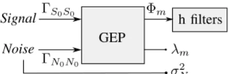
[12]. The classical SMF can be decomposed as a preprocessing stage as shown by Fig. 1 block diagram, followed with an on-line procedure illustrated in Fig. 2. According to Fig. 1,
GEP Signal Noise h filters S0S0 N0N0 m m 2 N
Fig. 1. Scheme of the SMF pre-processing.
Observation SNR 2 N m hQ[k] ˜ SQ[k][k] ⌦ h filters
Fig. 2. Scheme of the SMF on-line processing.
the method requires both signal and noise references for the preprocessing stage such as S0S0and N0N0, respectively the
signal’s and noise’s covariance matrices. These inputs are used in the following Generalized Eigenvalue Problem (GEP) [12]:
S0S0 m= m N0N0 m, (1)
to calculate the linear short band filter bank h using m
eigen-vectors as well as the meigenvalues. The current observation
Zk, where k denotes the sliding window’s index, and the
previously computed parameters, are then performed on-line to estimate the reconstructed observation ˜SQ[k][k](Fig. 2). It
is important to notice that here the key parameter, the time-dependent SNR ⇢k, is estimated from the power ratio
⇢k= 2 Zk 2N 2 N , (2)
providing the real-time parameter to choose how to filter Zk.
Since a low ⇢k indicates the absence of the signal in the
observation, it would realize the first filter selection only, inducing a strong filtering operation that cancels the noise. A contario, a high ⇢k, mirroring the presence of the signal,
would select the maximum number of filters: the operation would be then equivalent to a signal-bandpass filtering of the observation.
To conclude, the classical SMF requires :
- a background noise sample, long enough to be conside-red as a reference or an equivalent noise simulation, - a prior knowledge of the expected signal’s spectral
content and,
- SNR estimation tools.
III. IMPROVEDSMFFORZ-CALL PASSIVE DETECTION
While section II presents the classical theory of the SMF, it is introduced here as an innovative tool for Antarctic blue whale detection in a passive context. The signal reference is first adjusted to fit the problematic, then the background noise estimation is reassessed and a new time-varying SNR evaluation method is presented.
A. Signal’s reference: Antarctic blue whale call
Antarctic blue whale (Balaenoptera musculus intermedia) highly recognizable time-frequency call pattern, as presented in Fig 3b, gave it the name of Z-call. It consists of 3 short units composing the whole call lasting about 20 s, repeated about every 60 s in a phrase. Those phrases can occur from few minutes to several hours. Z-calls are composed from :
- unit A, the highest tonal part of the call with frequency between 25.5 and 27 Hz, lasting about 8 s,
- unit B, a ⇠ 2 s-long down sweep from unit A to C and, - unit C, a slightly modulated 8 s-long tone between 17
and 20 Hz.
Antarctic blue whale call levels in the Indian ocean have recently been evaluated for the [17 30] Hz frequency band at 179± 5 dB ref.1µPa@1 m [15]. According to Fig. 3a, unit A carries more energy than the rest of the call that causes differed arrival of acoustic paths producing Fig. 3b persisting ”trail” even after the down-sweep. Socheleau et al. [5] presented a
Z-15 20 25 30 Frequency (Hz) 0 0.5 1 Normalized Amp. (a) 0 100 200 300 Time (s) 10 20 30 40 Frequency (Hz) (b)
Fig. 3. Z-call: (a) spectrum showing unit A and C (b) spectrogram and parametric model with length of the Z-call TZcall = 20 s, fc =
22.6 Hz, L = [ 4.5; 4; 3.5] Hz, U = [3.2; 3.6; 4] Hz, M = [TZcall 2 ; (TZcall+0.5) 2 ; (TZcall+1) 2 ]s and ↵ = 1.8.
call parametric model, for frequency modulated signals, based on the complex form of an acoustic signal s(n) = a(n)ej'(n),
with a(n) the varying amplitude and '(n) the time-varying phase. From the definition of the instantaneous fre-quency and its parametric expression
f (t) = fc+ 1 2⇡ d'(t) dt = fc+ L + U L 1 + e↵(t M ), (3)
it is possible to derive the expression of the time-varying phase
'(n)as '(n) = 2⇡ ✓ Ln fs + U L ↵ ln ✓ 1 + e ↵M 1 + e↵(fsn M ) ◆◆ +'0, (4)
where fc is the central frequency in the [15 30]Hz
band-width, L and U are respectively linked to the lower and upper asymptotes, M represents the time shift and ↵ the grow rate. To generate the most accurate signal reference, providing for the different type of calls, it is simulated here as the summation of several frequency modulated signals, with parameters set as shown in Fig. 3b. This ”signature” is then used to compute
S0S0 as one of the input parameters of the GEP eq. (1).
B. Background noise estimation
Classical SMF noise estimation (§ II) rests on the strong assumptions that a portion of the observation can be signal-free. Although it is quite easy to manage when considering
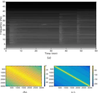
human-produced sounds e.g. active sonar emission, PAM does not benefit of the same ease. Useful signal can occur anytime. In this direction, an overall background noise estimation is realized using the outliers-smoothing properties of median filters. It is applied on each frequency canal of the K-lengthen observation’s Short-Time Fourier Transform (STFT) P (k, f), through a w sliding window of greater length than a call duration. The result is noted Pmed(k, f ). Considering the
60 min-long observation containing both signal of interest
and strong diverse noises displayed in Fig. 6a, the corres-ponding spectrogram |Pmed(k, f )|2 is plotted on Fig. 4a.
Resulting background noise covariance matrices estimation
N0N0before and after median filter application are displayed
in Fig. 4b and Fig. 4c respectively. It highlights that this stage is equivalent to a whitening of the noise [16].
0 10 20 30 40 50 60 Time (min) 0 5 10 15 20 25 30 35 40 45 50 Frequency (Hz) (a) 500 1000 1500 2000 2500 3000 500 1000 1500 2000 2500 3000 -80 -60 -40 -20 0 (b) 500 1000 1500 2000 2500 3000 500 1000 1500 2000 2500 3000 -200 -150 -100 -50 (c)
Fig. 4. Effect of the median filter on the background noise estimation when applied to the observation in Fig.6a. (a) |Pmed(k, f )|2 spectrogram, w =
65s, (b) Classical SMF N0N0, (c) Median filter SMF N0N0.
Considering classical SMF requirements, this processing stage is a step forward to a more autonomous method, by-passing the operator background noise selection: the SMF becomes suitable for passive detection. The whitening pro-cess provides a time-independent and robust computation of
N0N0. Since both inputs of the GEP (eq. (1)) are now fixed,
it is possible to realize a definitive off-line computation of the optimum filter bank with respect to the Z-call pattern. Fig. 5 illustrates the frequency response of filters H1, H10and
HQmax, where HQ denotes the superposition of the Q-first
filters of the linear filter bank denoted hQ in § II, compared
to the spectral representation HOpt of the signal’s reference (§ III-A). The first filter H1 is a short-band filter centered on
the call’s unit A (⇠ 26.3 Hz), containing most of the energy of the Z-call. As the theory demonstrates in § II, the role of the first filter is to maximize the output SNR; it cancels
the noise when the estimation of ⇢k indicates there is no
signal. The superposition of the first 10 filters H10 leads to
15 20 25 30 Frequency (Hz) 0 0.1 0.2 0.3 0.4 0.5 0.6 0.7 0.8 0.9 1 Normalized amplitude
Gabarit filtres : trad
H 1 H 10 H Qmax HOpt
Fig. 5. Spectrum of three filters (H1, H10, HQmax) of the permanent filter
bank compared to the spectral representation of the reference signal (HOpt).
two slightly larger bandpass filters, respectively centered on
units A (⇠ 18.6 Hz) and C (⇠ 26.3 Hz) of the call. HQmax
represents the superposition of the maximum number of filters that is applied when the estimated input ⇢k (see § III-C) is
high enough. The filter’s pattern is then close to HOpt. When applied, it bandpass filters the observation in the exact signal range. However, due to the influence of the background noise, amplitudes do not match completely the reference’s signature, especially between 22 Hz and 24 Hz, to maximize the output SNR.
Again, the passive approach with real marine noise requires some adjustments on the ⇢k evaluation to perform reliable
detection, as it is the well-known key parameter of the SMF. They are presented in § III-C.
C. Time-dependant SNR calculation
The time-varying input SNR ⇢k is used as a decision
criterion on the proper number of filters to apply to a Z observation. As a key parameter to the SMF, its estimate has to be accurate. Yet, its classical definition (eq. (2)) does not fit a low SNR passive context. To improve the sharpness of its estimation when dealing with real underwater noises and decrease the false alarm, ⇢k is completed with a frequency
criterion following Pmed(k, f )calculation. For every k
obser-vation sample, there are three different steps:
7! Step 1: The signal presence is quantified in the unit A of the call frequency band, as the ratio
zcallk= max f2AP (k, f ) 1 K K P k=1 Pmed(k, f0) , f02 A. (5)
Instantaneous value P (k, f) compared to Pmed(k, f )
indicates the presence of a short-duration signal in unit A frequency band as soon as the ratio is greater than one. However, it does not differentiate Z-calls from seismic noise.
7! Step 2: A background noise estimation is realized out of the frequency band of the Z-call as the ratio
transk= max f P (k, f ) Pmed(k, f ) , f 2 [0, inf(C)[[] sup(A),fs 2[. (6) aiming to prevent false alarm due to broadband noise.
7! Step 3: The time dependent SNR ⇢k, is then
deter-mined in dB as the ratio of (5) and (6) as ⇢k = 20 log ✓ zcallk transk ◆ . (7)
To perform detection, a threshold is applied to ⇢k for
whole observation (K) duration, depending on the background noise estimation as = ( 0 if M > 0 M elswise, (8) with M = 1 K K P k=1
(zcallk transk). Only positive values of
⇢k trigger the reconstruction of the observation.
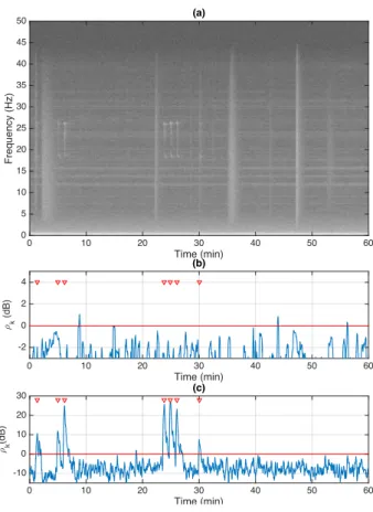
Fig. 6a is representative of OBSh signals revealing boat tonal noise that occurs for several hours with multiple har-monics and broadband seismic activity that covers the Z-call band. They last from few seconds to several minutes and carry high energy. Seven Z-calls can be noticed on the spectrogram however they are overlapped by seismic activity at 1.5 min and 30 min. There might be some (distant) other type of whale calls between 10 and 20 min.
Fig. 6 presents the difference between the former (eq. (2), Fig. 6b) and the new frequency dependent (eq. (7), Fig. 6c) estimation of ⇢k relative to the observation time-frequency
representation Fig. 6a. It highlights that the original calculation of ⇢k (eq. (2)) does not achieve the expected operation: in
comparison to e.g. seismic broadband noise, the presence of Z-calls does not significantly increase its estimated instantaneous
level. Consequently, the SMF using this estimation of ⇢k
would not fit a passive detection problem with no signal excess. However, the new method based on the median-filtered STFT and introducing a frequency-dependence, increases the ⇢k on Z-calls but not on seismic noises. It is more suitable
to trigger detection even at low average SNR due to high background noise environment or distant calls. The frequency discrimination reduces the probability of false alarm and increases the detection probability.
Basically, the main improvements to the SMF are:
- the expected signal’s time-frequency pattern is known and modeled,
- no more need for background noise selection due to the observation’s median-filter whitening and,
- the time-dependent SNR ⇢k estimation is revised by
time-frequency analysis.
In addition, changes on signal and noise references, lead to an off-line calculation of a generalized h-filter bank that is more robust and enhances the computational time.
(a) 0 10 20 30 40 50 60 Time (min) 0 5 10 15 20 25 30 35 40 45 50 Frequency (Hz) 0 10 20 30 40 50 60 Time (min) -2 0 2 4 ;k (dB) (b) 0 10 20 30 40 50 60 Time (min) -10 0 10 20 30 ;k (dB) (c)
Fig. 6. (a) Spectrogram of the considered observation with |P (k, f)|2
N f f t = 2048 and overlap = 95%. Broadband noise correspond to earthquakes and tonal noise to ship noise. (b) & (c) Former and new time varying SNR calculation. Visually checked Z-calls are denoted by red markers.
Now that every step of the SMF is optimized for a robust detection of Z-calls in a passive context, section IV presents a way to use the output of the SMF for calls time of arrival estimation.
IV. TIME OF ARRIVAL CALCULATION
Input and output of the SMF can be compared in Fig. 7a. On the SMF output, the observation is fully reconstructed in the signal’s bandwidth (Fig. 5) for every marked Z-call despite broadband seismic noises. It stresses both the influence of the accurate estimation of ⇢k and the noise-canceling property
of the first filter. Fig. 7b displays the correlation maximum (Corr.max) between the windowed input observation and the
signal’s reference described in § III-A, noted MF. It is to be compared with Fig. 7c, the correlation maximum between the windowed output of the SMF and the signal’s reference, noted SMF + MF. Both of these results are plotted normalized so that the maximum, the reference signal autocorrelation, is 1. Since in both cases, 100% of Z-calls are detected, the false alarm rate that is used to point up the benefit of the SMF: if a threshold is set at 0.007 in Fig. 7b, 4 peaks are due to the seismic noise at the MF output whereas the SMF + MF output Fig. 7c does not generate false alarm. In addition of being able to compare the results with the classical MF method, using correlation at the
0 10 20 30 40 50 60 Time (min) -0.3 -0.2 -0.1 0 0.1 0.2 Norm. Amp. (a) SMF input SMF output 0 10 20 30 40 50 60 Time (min) 0 0.02 0.04 0.06 Corr. max MF (b) 0 10 20 30 40 50 60 Time (min) 0 0.05 0.1 0.15 0.2 Corr. max SMF + MF (c)
Fig. 7. (a) SMF input and output normalized by the input maximum. Maximum correlation between [the input observation (b), and SMF output (c)] and the signal’s reference over a sliding window. Correlation values are normalized by the reference signal. Z-calls are denoted by the red markers.
output of the SMF to create detection peaks can be useful for similarities measurements. Also, it provides a systematic call time of arrival estimation, first step to a multi-sensor approach, to discriminate different whales paths for individual tracking that can lead to an estimation of individuals in the region.
V. CONCLUSION
Several SMF improvements are presented to suit passive detection of Antarctic blue whale Z-calls in noisy underwa-ter environment. The signal’s reference [5] is updated from spectrogram-analyzed OBSh data. A new method for back-ground noise estimation, based on the observation’s median-filtered STFT, bypasses the selection by an operator. As it is assimilated to a whitening process, now both necessary inputs loose their time dependency resulting in a definitive off-line evaluation of the SMF’s linear filter bank. The key parameter estimation of the time-varying SNR ⇢k is revised
from time-frequency analysis, with a frequency criterion that reduces false alarms in presence of broadband high energy seismic noise. Each step of the method’s changes is illustrated to result in an application on a really noisy observation. The new SMF’s output correlated with the signal’s reference is then compared to the MF, showing greater robustness to impulsive noise and drastic false alarm reduction. It can also be used
to measure similarities and determine call-time of arrivals, providing new opportunities for automatic source localizations and whale tracking. Next stage to this work is to evaluate the method in terms of performances (ROC and performance curves) by applying it to marked observations with different background noise environments, including other types of calls or in presence of distant Z-calls.
ACKNOWLEDGMENT
The RHUM-RUM project [17],[18] was funded by ANR (Agence Nationale de la Recherche) in France (project ANR-11-BS56-0013), and by DFG (Deutsche Forschungsgemein-schaft) in Germany.
REFERENCES
[1] R. A. Dunn and O. Hernandez, “Tracking blue whales in the eastern tropical pacific with an ocean-bottom seismometer and hydrophone array,” J. Acoust. Soc. Am., vol. 126, no. 3, pp. 1084–1094, 2009. [2] M. A. McDonald, S. L. Mesnick, and J. A. Hildebrand, “Biogeographic
characterization of blue whale song worldwide: Using song to identify populations,” Journal of Cetacean Research and Management, vol. 8, no. 1, pp. 55–65, 2006.
[3] N. E. Balcazar, J. S. Tripovich, H. Klinck, S. L. Nieukirk, D. K. Mellinger, R. P. Dziak, and T. L. Rogers, “Calls reveal population structure of blue whales across the southeast indian ocean and southwest pacific ocean,” Journal of Mammalogy, vol. 96, no. 6, pp. 1184, 2015. [4] F. Samaran, O. Adam, and C. Guinet, “Detection range modeling of blue whale calls in Southwestern Indian Ocean,” Applied Acoustics, vol. 71, no. 11, pp. 1099–1106, 2010.
[5] F.-X. Socheleau, E. Leroy, A. Carvallo Pecci, F. Samaran, J. Bonnel, and J.-Y. Royer, “Automated detection of antarctic blue whale calls,” J. Acoust. Soc. Am., vol. 138, no. 5, pp. 3105–3117, 2015.
[6] E. C. Leroy, F. Samaran, J. Bonnel, and J.-Y. Royer, “Seasonal and diel vocalization patterns of antarctic blue whale (balaenoptera musculus intermedia) in the southern indian ocean: A multi-year and multi-site study,” PLOS ONE, vol. 11, no. 11, pp. 1–20, 2016.
[7] S. D. Frank and A. N. Ferris, “Analysis and localization of blue whale vocalizations in the solomon sea using waveform amplitude data,” J. Acoust. Soc. Am., vol. 130, no. 2, pp. 731–736, 2011.
[8] D. Harris, L. Matias, L. Thomas, J. Harwood, and W. H. Geissler, “Applying distance sampling to fin whale calls recorded by single seismic instruments in the northeast atlantic,” J. Acoust. Soc. Am., vol. 134, no. 5, pp. 3522–3535, 2013.
[9] G. Barruol, K. Sigloch, and RHUM-RUM group, “RHUM-RUM experiment, 20112015, code YV (R´eunion Hotspot and Upper Mantle -R´eunion’s Unterer Mantel) funded by ANR, DFG, CNRS-INSU, IPEV, TAAF, instrumented by DEPAS, INSU-OBS, AWI and the Universities of Muenster, Bonn, La R´eunion,” 2017.
[10] G. Barruol and K. Sigloch, “Investigating la r´eunion hot spot from crust to core,” Eos, Transactions American Geophysical Union, vol. 94, no. 23, pp. 205–207, 6 2013.
[11] J-F. Cavassillas, “Stochastic matched filter,” Proc. Institute of Acoustics (Int. Conf. Sonar Signal Processing), vol. 13, part. 9, pp. 194–199, 1991. [12] P. Courmontagne, G. Julien, and M.E. Bouhier, “An improvement to the pulse compression scheme,” in OCEANS 2010 IEEE - Sydney, 2010, pp. 1–5.
[13] F. Caudal and H. Glotin, “Stochastic Matched Filter outperforms Teager-Kaiser-Mallat for tracking a plurality of sperm whales,” New Trends for Environmental Monitoring Using Passive Systems, 2008, pp. 1–9, 2008. [14] J. Bonnal, P. Danes, and M. Renaud, “Detection of acoustic patterns by stochastic matched filtering,” in Int. Conf. Intelligent Robots and Systems, 2010, pp. 1970–1975.
[15] F. Samaran, C. Guinet, O. Adam, J.-F. Motsch, and Y. Cansi, “Source level estimation of two blue whale subspecies in southwestern indian ocean,” J. Acoust. Soc. Am., vol. 127, no. 6, pp. 3800–3808, 2010. [16] H. L. Van Trees, Optimum Array Processing: Part IV of Detection,
Estimation, and Modulation Theory, John Wiley and Sons, Inc., 2002. [17] “Rhum-rum web page,” www.rhum-rum.net.