HAL Id: hal-00344222
https://hal.archives-ouvertes.fr/hal-00344222
Submitted on 4 Dec 2008
HAL is a multi-disciplinary open access
archive for the deposit and dissemination of
sci-entific research documents, whether they are
pub-lished or not. The documents may come from
teaching and research institutions in France or
abroad, or from public or private research centers.
L’archive ouverte pluridisciplinaire HAL, est
destinée au dépôt et à la diffusion de documents
scientifiques de niveau recherche, publiés ou non,
émanant des établissements d’enseignement et de
recherche français ou étrangers, des laboratoires
publics ou privés.
games as limits of multi-discounted game
Hugo Gimbert, Wieslaw Zielonka
To cite this version:
Hugo Gimbert, Wieslaw Zielonka. Applying Blackwell optimality: priority mean-payoff games as
limits of multi-discounted game. Texts in Logic and Games, 2007, 2, pp.331-356. �hal-00344222�
Applying Blackwell Optimality: Priority
Mean-Payoff Games as Limits of Multi-Discounted
Games
Hugo Gimbert
1Wies!law Zielonka
2∗ 1LIX, ´Ecole Polytechnique, Palaiseau, France
2
Universit´e Denis Diderot and CNRS, LIAFA case 7014, 75205 Paris Cedex 13, France
[email protected] [email protected]
Abstract
We define and examine priority mean-payoff games — a natural extension of parity games. By adapting the notion of Blackwell op-timality borrowed from the theory of Markov decision processes we show that priority mean-payoff games can be seen as a limit of special multi-discounted games.
1
Introduction
One of the major achievements of the theory of stochastic games is the re-sult of Mertens and Neyman [15] showing that the values of mean-payoff games are the limits of the values of discounted games. Since the limit of the discounted payoff is related to Abel summability while the mean-payoff is related to Ces`aro summability of infinite series, and classical abelian and tauberian theorems establish tight links between these two summability methods, the result of Mertens and Neyman, although technically very dif-ficult, comes with no surprise.
In computer science similar games appeared with the work of Gurevich and Harrington [12] (games with Muller condition) and Emerson and Jutla [5] and Mostowski [16] (parity games).
However discounted and mean-payoff games also seem very different from Muller/parity games. The former, inspired by economic applications, are games with real valued payments, the latter, motivated by logics and au-tomata theory, have only two outcomes, the player can win or lose.
The theory of parity games was developed independently from the the-ory of discounted/mean-payoff games [11] even though it was noted by
dzi´nski [14] that deterministic parity games on finite arenas can be reduced to mean-payoff games1.
Recently de Alfaro, Henzinger and Majumdar [3] presented results that indicate that it is possible to obtain parity games as an appropriate limit of multi-discounted games. In fact, the authors of [3] use the language of the µ-calculus rather than games, but as the links between µ-calculus and parity games are well-known since the advent [5], it is natural to wonder how discounted µ-calculus from [3] can be reflected in games.
The aim of this paper is to examine in detail the links between discounted and parity games suggested by [3]. In our study we use the tools and methods that are typical for classical game theory but nearly never used for parity games. We want to persuade the reader that such tools, conceived for games inspired by economic applications, can be successfully applied to games that come from computer science.
As a by-product we obtain a new class of games — priority mean-payoff games — that generalise in a very natural way parity games but contrary to the latter allow to quantify the gains and losses of the players.
The paper is organised as follows.
In Section 2 we introduce the general framework of deterministic zero-sum infinite games used in the paper, we define optimal strategies, game values and introduce positional (i.e. memoryless) strategies.
In Section 3 we present discounted games. Contrary to classical game theory where there is usually only one discount factor, for us it is crucial to work with multi-discounted games where the discount factor can vary from state to state.
Section 4 is devoted to the main class of games examined in this paper — priority mean-payoff games. We show that for these games both players have optimal positional strategies (on finite arenas).
In classical game theory there is a substantial effort to refine the notion of optimal strategies. To this end Blackwell [2] defined a new notion of op-timality that allowed him a fine-grained classification of optimal strategies for mean-payoff games. In Section 5 we adapt the notion of Blackwell op-timality to our setting. We use Blackwell opop-timality to show that in some strong sense priority mean-payoff games are a limit of a special class of multi-discounted games.
The last Section 6 discusses briefly some other applications of Blackwell optimality.
Since the aim of this paper is not only to present new results but also to familiarize the computer science community with methods of classical game theory we have decided to make this paper totally self-contained. We present
1
But this reduction seems to be proper for deterministic games and not possible for perfect information stochastic games.
2. GAMES 3
all proofs, even the well-known proof of positionality of discounted games2.
For the same reason we also decided to limit ourselves to deterministic games. Similar results can be proved for perfect information stochastic games [10, 9] but the proofs become much more involved. We think that the deterministic case is still of interest and has the advantage of beeing accessible through elementary methods.
The present paper is an extended and improved version of [8].
2
Games
An arena is a tuple A = (S1, S2, A), where S1 and S2are the sets of states
that are controlled respectively by player 1 and player 2, A is the set of actions.
By S = S1 ∪ S2 we denote the set of all states. Then A ⊆ S × S,
i.e. each action a = (s!, s!!) ∈ A is a couple composed of the source state
source(a) = s! and the target state target(a) = s!!. In other words, an arena
is just as a directed graph with the set of vertices S partitioned onto S1and
S2 with A as the set of edges.
An action a is said to be available at state s if source(a) = s and the set of all actions available at s is denoted by A(s).
We consider only arenas where the set of states is finite and such that for each state s the set A(s) of available actions is non-empty.
A path in arena A is a finite or infinite sequence p = s0s1s2. . . of states
such that ∀i, (si, si+1) ∈ A. The first state is the source of the p, source(p) =
s0, if p is finite then the last state is the target of p, target(p).
Two players 1 and 2 play on A in the following way. If the current state s is controlled by player P ∈ {1, 2}, i.e. s ∈ SP, then player P chooses an
action a ∈ A(s) available at s, this action is executed and the system goes to the state target(a).
Starting from an initial state s0, the infinite sequence of consecutive
moves of both players yields an infinite sequence p = s0s1s2. . . of visited
states. Such sequences are called plays, thus plays in this game are just infinite paths in the underlying arena A.
We shall also use the term “a finite play” as a synonym of “a finite path” but “play” without any qualifier will always denote an infinite play/path.
A payoff mapping
u : Sω→ R (1.1)
maps infinite sequences of states to real numbers. The interpretation is that at the end of a play p player 1 receives from player 2 the payoff u(p) (if
2
But this can be partially justified since we need positionality of multi-discounted games while in the literature usually simple discounted games are treated. We should admit however that passing from discounted to multi-discounted games needs only minor obvious modifications.
u(p) < 0 then it is rather player 2 that receives from player 1 the amount |u(p)|).
A game is couple (A, u) composed of an arena and a payoff mapping. The obvious aim of player 1 (the maximizer) in such a game is to maxi-mize the received payment, the aim of player 2 (the minimaxi-mizer) is opposite, he wants to minimize the payment paid to his adversary.
A strategy of a player P is his plan of action that tells him which action to take when the game is at a state s ∈ SP. The choice of the action can
depend on the whole past sequence of moves. Therefore a strategy for player 1 is a mapping
σ : {p | p a finite play with target(p) ∈ S1} −→ S (1.2)
such that for each finite play p with s = target(p) ∈ S1, (s, σ(p)) ∈ A(s).
Strategy σ of player 1 is said to be positional if for every state s ∈ S1
and every finite play p with target(p) = s, σ(p) = σ(s). Thus the action chosen by a positional strategy depends only on the current state, previously visited states are irrelevant. Therefore a positional strategy of player 1 can be identified with a mapping
σ : S1→ S (1.3)
such that ∀s ∈ S1, (s, σ(s)) ∈ A(s).
A finite or infinite play p = s0s1. . . is said to be consistent with a
strategy σ of player 1 if, for each i ∈ N such that si ∈ S1, we have
(si, σ(s0. . . si−1)) ∈ A.
Strategies, positional strategies and consistent plays are defined in the analogous way for player 2 with S2replacing S1.
In the sequel Σ and T will stand for the set of strategies for player 1 and player 2 while Σpand Tpare the corresponding sets of positional strategies.
The letters σ and τ , with subscripts or superscripts if necessary, will be used to denote strategies of player 1 and player 2 respectively.
Given a pair of strategies σ ∈ Σ and τ ∈ T and an initial state s, there exists a unique infinite play in arena A, denoted p(s, σ, τ ), consistent with σ and τ and such that s = source(p(s, σ, τ )).
Definition 2.1. Strategies σ" ∈ Σ and τ" ∈ T are optimal in the game
(A, u) if
∀s ∈ S, ∀σ ∈ Σ, ∀τ ∈ T ,
2. GAMES 5
Thus if strategies σ" and τ" are optimal then the players do not have
any incentive to change them unilaterally: player 1 cannot increase his gain by switching to another strategy σ while player 2 cannot decrease his losses by switching to another strategy τ .
In other words if player 2 plays according to τ" then the best response
of player 1 is to play with σ", no other strategy can do better for him.
Conversely, if player 1 plays according to σ"then the best response of player
2 is to play according to τ"as no other strategy does better to limit his losses.
We say that a payoff mapping u admits optimal positional strategies if for all games (A, u) over finite arenas there exist optimal positional strategies for both players. We should emphasize that the property defined above is a property of the payoff mapping and not a property of a particular game, we require that both players have optimal positional strategies for all possible games over finite arenas.
It is important to note that zero-sum games that we consider here, i.e. the games where the gain of one player is equal to the loss of his adversary, satisfy the exchangeability property for optimal strategies:
for any two pairs of optimal strategies (σ", τ") and (σ#, τ#), the pairs
(σ#, τ") and (σ", τ#) are also optimal and, moreover,
u(p(s, σ", τ")) = u(p(s, σ#, τ#)) ,
i.e. the value of u(p(s, σ", τ")) is independent of the choice of the optimal
strategies — this is the value of the game (A, u) at state s. We end this general introduction with two simple lemmas.
Lemma 2.2. Let u be a payoff mapping admitting optimal positional strategies for both players.
(A) Suppose that σ ∈ Σ is any strategy while τ"∈ T
p is positional. Then
there exists a positional strategy σ"∈ Σ
p such that
∀s ∈ S, u(p(s, σ, τ")) ≤ u(p(s, σ", τ")) . (1.5) (B) Similarly, if τ ∈ T is any strategy and σ" ∈ Σ
p a positional strategy
then there exists a positional strategy τ"∈ T
p such that
∀s ∈ S, u(p(s, σ", τ")) ≤ u(p(s, σ", τ )) .
Proof. We prove (A), the proof of (B) is similar. Take any strategies σ ∈ Σ and τ"∈ T
p. Let A! be a subarena of A obtained by restricting the actions
of player 2 to the actions given by the strategy τ", i.e. in A! the only
not restricted, i.e. in A! player 1 has the same available actions as in A, in
particular σ is a valid strategy of player 1 on A!. Since u admits optimal
positional strategies, player 1 has an optimal positional strategy σ" on A!.
But (1.5) is just the optimality condition of σ" on A!.
q.e.d.
Lemma 2.3. Suppose that the payoff mapping u admits optimal positional strategies. Let σ"∈ Σ
p and τ"∈ Tpbe positional strategies such that
∀s ∈ S, ∀σ ∈ Σp, ∀τ ∈ Tp,
u(p(s, σ, τ")) ≤ u(p(s, σ", τ") ≤ u(p(s, σ", τ )) , (1.6) i.e. σ" and τ"are optimal in the class of positional strategies. Then σ"and
τ"are optimal in the class of all strategies.
Proof. Suppose that
∃τ ∈ T , u(p(s, σ", τ )) < u(p(s, σ", τ")) . (1.7)
By Lemma 2.2 (B) there exists a positional strategy τ# ∈ T
p such that
u(p(s, σ", τ#)) ≤ u(p(s, σ", τ )) < u(p(s, σ", τ")), contradicting (1.6). Thus
∀τ ∈ T , u(p(s, σ", τ")) ≤ u(p(s, σ", τ )). The left hand side of (1.4) can be
proved in a similar way. q.e.d.
3
Discounted Games
Discounted games where introduced by Shapley [19] who proved that stochas-tic discounted games admit stationary optimal strategies. Our exposition follows very closely the original approach of [19] and that of [17]. Neverthe-less we present a complete proof for the sake of completeness.
Arenas for discounted games are equipped with two mappings defined on the set S of states: the discount mapping
λ : S −→ [0, 1)
associates with each state s a discount factor λ(s) ∈ [0, 1) and the reward mapping
r : S −→ R (1.8)
maps each state s to a real valued reward r(s). The payoff mapping
uλ: Sω−→ R
for discounted games is defined in the following way: for each play p = s0s1s2. . . ∈ Sω uλ(p) = (1 − λ(s0))r(s0) + λ(s0)(1 − λ(s1))r(s1) + λ(s0)λ(s1)(1 − λ(s2))r(s2) + . . . = ∞ ! i=0 λ(s0) . . . λ(si−1)(1 − λ(si))r(si) . (1.9)
3. DISCOUNTED GAMES 7
Usually when discounted games are considered it is assumed that there is only one discount factor, i.e. that there exists λ ∈ [0, 1) such that λ(s) = λ for all s ∈ S. But for us it is essential that discount factors depend on the state.
It is difficult to give an intuitively convincing interpretation of (1.9) if we use this payoff mapping to evaluate infinite games. However, there is a natural interpretation of (1.9) in terms of stopping games, in fact this is the original interpretation given by Shapley[19].
In stopping games the nature introduces an element of uncertainty. Sup-pose that at a stage i a state siis visited. Then, before the player controlling
si is allowed to execute an action, a (biased) coin is tossed to decide if the
game stops or if it will continue. The probability that the game stops is 1 − λ(si) (thus λ(si) gives the probability that the game continues). Let
us note immediately that since we have assumed that 0 ≤ λ(s) < 1 for all s ∈ S, the stopping probabilities are strictly positive therefore the game actually stops with probability 1 after a finite number of steps.
If the game stops at si then player 1 receives from player 2 the payment
r(si). This ends the game, there is no other payment in the future.
If the game does not stop at si then there is no payment at this stage
and the player controlling the state si is allowed to choose an action to
execute3.
Now note that λ(s0) . . . λ(si−1)(1 − λ(si)) is the probability that the
game have not stopped at any of the states s0, . . . , si−1 but it does stop at
state si. Since this event results in the payment r(si) received by player 1,
Eq. (1.9) gives in fact the payoff expectation for a play s0s1s2. . ..
Shapley [19] proved4 that
Theorem 3.1 (Shapley). Discounted games (A, uλ) over finite arenas
ad-mit optimal positional strategies for both players.
Proof. Let RS be the vector space consisting of mappings from S to R. For
f ∈ RS, set ||f || = sup
s∈S|f (s)|. Since S is finite || · || is a norm for which
RS is complete. Consider an operator Ψ : RS −→ RS, for f ∈ RS and
s ∈ S,
Ψ[f ](s) = "
max(s,s!)∈A(s)(1 − λ(s))r(s) + λ(s)f (s!) if s ∈ S1
min(s,s!)∈A(s)(1 − λ(s))r(s) + λ(s)f (s!) if s ∈ S2 .
Ψ[f ](s) can be seen as the value of a one shot game that gives the payoff (1−λ(s))r(s)+λ(s)f (s!) if the player controlling the state s choses an action
(s, s!) ∈ A(s). 3
More precisely, if the nature does not stop the game then the player controlling the current state is obliged to execute an action, players cannot stop the game by them-selves.
4
We can immediately note that Ψ is monotone, if f ≥ g then Ψ[f ] ≥ Ψ[g], where f ≥ g means that f (s) ≥ g(s) for all states s ∈ S.
Moreover, for any positive constant c and f ∈ RS
Ψ[f ] − cλ1 ≤ Ψ[f − c · 1] and Ψ[f + c · 1] ≤ Ψ[f ] + cλ1 , (1.10) where 1 is the constant mapping, 1(s) = 1 for each state s, and λ = sups∈Sλ(s). Therefore, since f − ||f − g|| · 1 ≤ g ≤ f + ||f − g|| · 1 , we get Ψ[f ] − λ||f − g|| · 1 ≤ Ψ[g] ≤ Ψ[f ] + λ||f − g|| · 1 , implying ||Ψ[f ] − Ψ[g]|| ≤ λ||f − g|| .
By Banach contraction principle, Ψ has a unique fixed point w ∈ RS,
Ψ[w] = w. From the definition of Ψ we can see that this unique fixed point satisfies the inequalities
∀s ∈ S1, ∀(s, s!) ∈ A(s), w(s) ≥ (1 − λ(s))r(s) + λ(s)w(s!) (1.11)
and
∀s ∈ S2, ∀(s, s!) ∈ A(s), w(s) ≤ (1 − λ(s))r(s) + λ(s)w(s!) . (1.12)
Moreover, for each s ∈ S there is an action ξ(s) = (s, s!) ∈ A(s) such that
w(s) = (1 − λ(s))r(s) + λ(s)w(s!) . (1.13)
We set σ"(s) = ξ(s) for s ∈ S
1 and τ"(s) = ξ(s) for s ∈ S2 and we show
that σ" and τ" are optimal for player 1 and 2. Suppose that player 1 plays
according to the strategy σ"while player 2 according to some strategy τ . Let
p(s0, σ", τ ) = s0s1s2. . .. Then, using (1.12) and (1.13), we get by induction
on k that w(s0) ≤ k ! i=0 λ(s0) . . . λ(si−1)(1 − λ(si))r(si) + λ(s0) . . . λ(sk)w(sk+1) .
Tending k to infinity we get
w(s0) ≤ uλ(p(s0, σ", τ )) .
In a similar way we can establish that for any strategy σ of player 1, w(s0) ≥ uλ(p(s0, σ, τ"))
and, finally, that
w(s0) = uλ(p(s0, σ", τ")) ,
4. PRIORITY MEAN-PAYOFF GAMES 9
4
Priority mean-payoff games
In mean-payoff games the players try to optimize (maximize/minimize) the mean value of the payoff received at each stage. In such games the reward mapping
r : S −→ R (1.14)
gives, for each state s, the payoff received by player 1 when s is visited. The payoff of an infinite play is defined as the mean value of daily payments:
um(s0s1s2. . .) = lim sup k 1 k + 1 k ! i=0 r(si) , (1.15)
where we take lim sup rather than the simple limit since the latter may not exist. As proved by Ehrenfeucht and Mycielski [4], such games admit optimal positional strategies; other proofs can be found for example in [1, 7]. We slightly generalize mean-payoff games by equipping arenas with a new mapping
w : S −→ R+ (1.16)
associating with each state s a strictly positive real number w(s), the weight of s. We can interpret w(s) as the amount of time spent at state s each time when s is visited. In this setting r(s) should be seen as the payoff by a time unit when s is visited, thus the mean payoff received by player 1 is
um(s0s1s2. . .) = lim sup k #k i=0w(si)r(si) #k i=0w(si) . (1.17)
Note that in the special case when the weights are all equal to 1, the weighted mean value (1.17) reduces to (1.15).
As a final ingredient we add to our arena a priority mapping
π : S −→ Z+ (1.18)
giving a positive integer priority π(s) of each state s.
We define the priority of a play p = s0s1s2. . . as the smallest priority
appearing infinitely often in the sequence π(s0)π(s1)π(s2) . . . of priorities
visited in p:
π(p) = lim inf
i π(si) . (1.19)
For any priority a, let 1a: S −→ {0, 1} be the indicator function of the set
{s ∈ S | π(s) = a}, i.e.
1a(s) =
"
1 if π(s) = a
Then the priority mean payoff of a play p = s0s1s2. . . is defined as upm(p) = lim sup k #k i=01π(p)(s) · w(si) · r(si) #k i=01π(p)(si) · w(si) . (1.21) In other words, to calculate priority mean payoff upm(p) we take weighted
mean payoff but with the weights of all states having priorities different from π(p) shrunk to 0. (Let us note that the denominator#k
i=01π(p)(si) · w(si)
is different from 0 for k large enough, in fact it tends to infinity since 1π(p)(si) = 1 for infinitely many i. For small k the numerator and the
denominator can be equal to 0 and then, to avoid all misunderstanding, it is convenient to assume that the indefinite value 0/0 is equal to −∞.)
Suppose that for all states s,
• w(s) = 1 and
• r(s) is 0 if π(s) is even, and r(s) is 1 if π(s) is odd.
Then the payoff obtained by player 1 for any play p is either 1 if π(p) is odd, or 0 if π(p) is even. If we interpret the payoff 1 as the victory of player 1, and payoff 0 as his defeat then such a game is just the usual parity game [5, 11].
It turns out that
Theorem 4.1. For any arena A the priority mean-payoff game (A, upm)
admits optimal positional strategies for both players.
There are many possible ways to prove Theorem 4.1, for example by adapting the proofs of positionality of mean payoff games from [4] and [1] or by verifying that upm satisfies sufficient positionality conditions given in
[7]. Below we give a complete proof based mainly on ideas from [7, 20]. A payoff mapping is said to be prefix independent if for each play p and for each factorization p = xy with x finite we have u(p) = u(y), i.e. the payoff does not depend on finite prefixes of a play. The reader can readily persuade herself that the priority mean payoff mapping upmis prefix
independent.
Lemma 4.2. Let u be a prefix-independent payoff mapping such that both players have optimal positional strategies σ"and τ"in the game (A, u). Let
val(s) = p(s, σ", τ"), s ∈ S, be the game value for an initial state s.
For any action (s, t) ∈ A, (1) if s ∈ S1 then val(s) ≥ val(t),
(2) if s ∈ S2 then val(s) ≤ val(t),
4. PRIORITY MEAN-PAYOFF GAMES 11
(4) if s ∈ S2 and τ"(s) = t then val(s) = val(t).
Proof. (1) This is quite obvious. If s ∈ S1, (s, t) ∈ A and val(s) < val(t)
then for a play starting at s player 1 could secure for himself at least val(t) by executing first the action (s, t) and next playing with his optimal strategy. But this contradicts the definition of val(s) since from s player 2 has a strategy that limits his losses to val(s).
The proof of (2) is obviously similar.
(3) We know by (1) that if s ∈ S1 and σ"(s) = t then val(s) ≥ val(t).
This inequality cannot be strict since from t player 2 can play in such a way that his loss does not exceed val(t).
(4) is dual to (1).
q.e.d.
Proof of Theorem 4.1. We define the size of an arena A to be the difference |A| − |S| of the number of actions and the number of states and we carry the proof by induction on the size of A. Note that since for each state there is at least one available action the size of each arena is ≥ 0.
If for each state there is only one available action then the number of actions is equal to the number of states, the size of A is 0, and each player has just one possible strategy, both these strategies are positional and, obviously, optimal.
Suppose that both players have optimal positional strategies for arenas of size < k and let A be of size k, k ≥ 1.
Then there exists a state with at least two available actions. Let us fix such a state t, we call it the pivot. We assume that t is controlled by player 1
t ∈ S1 (1.22)
(the case when it is controlled by player 2 is symmetric).
Let A(t) = AL(t)∪AR(t) be a partition of the set A(t) of actions available
at t onto two disjoint non-empty sets. Let AL and AR be two arenas, we
call them left and right arenas, both of them having the same states as A, the same reward, weight and priority mappings and the same available actions for all states different from t. For the pivot state t, AL and AR
have respectively AL(t) and AR(t) as the sets of available actions. Thus,
since AL and AR have less actions than A, their size is smaller than the
size of A and, by induction hypothesis, both players have optimal positional strategies: (σL", τL") on AL and (σR", τ
"
R) on AR.
We set valL(s) = upm(p(s, σL", τL")) and valR(s) = upm(p(s, σR", τR")) to
be the values of a state s respectively in the left and the right arena. Without loss of generality we can assume that for the pivot state t
We show that this implies that
∀s ∈ S, valL(s) ≤ valR(s) . (1.24)
Suppose the contrary, i.e. that the set
X = {s ∈ S | valL(s) > valR(s)}
is non-empty. We define a positional strategy σ∗ for player 1
σ∗(s) = "
σL"(s) if s ∈ X ∩ S1
σR"(s) if s ∈ (S \ X) ∩ S1.
(1.25) Note that, since the pivot state t does not belong to X, for s ∈ X ∩ S1,
σL"(s) is valid action for player 1 not only in AL but also in AR, therefore
the strategy σ∗defined above is a valid positional strategy on the arena A R.
We claim that
For games on AR starting at a state s0∈ X strategy σ∗ guarantees that
player 1 wins at least valL(s0) (against any strategy of player 2).
(1.26) Suppose that we start a game on AR at a state s0 and player 1 plays
according to σ∗ while player 2 uses any strategy τ . Let
p(s0, σ∗, τ ) = s0s1s2. . . (1.27)
be the resulting play. We define ∀s ∈ S, val(s) =
"
valL(s) for s ∈ X,
valR(s) for s ∈ S \ X.
(1.28) We shall show that the sequence val(s0), val(s1), val(s2), . . . is non-decreasing,
∀i, val(si) ≤ val(si+1) . (1.29)
Since strategies σL" and σR" are optimal in AL and AR, Lemma 4.2 and
(1.28) imply that for all i
val(si) = valL(si) ≤ valL(si+1) if si∈ X, (1.30)
and
val(si) = valR(si) ≤ valR(si+1) if si∈ S \ X. (1.31)
4. PRIORITY MEAN-PAYOFF GAMES 13
(1) Suppose that siand si+1belong to X. Then val(si+1) = valL(si+1) and
(1.29) follows from (1.30).
(2) Suppose that siand si+1 belong to S \ X. Then val(si+1) = valR(si+1)
and now (1.29) follows from (1.31).
(3) Let si∈ X and si+1∈ S \ X. Then (1.29) follows from (1.30) and from
the fact that valL(si+1) ≤ valR(si+1) = val(si+1).
(4) Let si∈ S \X and si+1∈ X. Then valR(si+1) < valL(si+1) = val(si+1),
which, by (1.31), implies (1.29). Note that in this case we have the strict inequality val(si) < val(si+1).
This terminates the proof of (1.29).
Since the set {val(s) | s ∈ S} is finite (1.29) implies that the sequence val(si), i = 0, 1, . . . , ultimately constant. But examining the case (4) above
we have established that each passage from S \ X to X strictly increases the value of val. Thus from some stage n onward all states si, i ≥ n, are either
in X or in S \ X. Therefore, according to (1.25), from the stage n onward player 1 always plays either σL" or σ"Rand the optimality of both strategies assures that he wins at least val(sn), i.e.
upm(p(s0, σ∗, τ )) = upm(s0s1. . .) = upm(snsn+1sn+2. . .) ≥ val(sn) ≥ val(s0).
In particular, if s0∈ X then using strategy σ∗ player 1 secures for himself
the payoff of at least val(s0) = valL(s0) against any strategy of player
2, which proves (1.26). On the other hand, the optimality of τR" implies that player 2 can limit his losses to valR(s0) by using strategy τR". But how
player 1 can win at least valL(s0) while player 2 loses no more than valR(s0)
if valL(s0) > valR(s0) for s0 ∈ X? We conclude that the set X is empty
and (1.24) holds.
Now our aim is to prove that (1.23) implies that the strategy σ"R is optimal for player 1 not only in AR but also for games on the arena A.
Clearly player 1 can secure for himself the payoff of at least valR(s) by
playing according to σ"R on A. We should show that he cannot do better. To this end we exhibit a strategy τ" for player 2 that limits the losses of
player 2 to valR(s) on the arena A.
At each stage player 2 will use either his positional strategy τL" optimal in AL or strategy τR" optimal in AR. However, in general neither of these
strategies is optimal for him in A and thus it is not a good idea for him to stick to one of these strategies permanently, he should rather adapt his strategy to the moves of his adversary. To implement the strategy τ"player
2 will need one bit of memory (the strategy τ" we construct here is not
the pivot state t player 1 took an action of AL(t) or an action of AR(t). In
the former case player 2 plays using the strategy τL", in the latter case he plays using the strategy τR". In the periods between two passages through t player 2 does not change his strategy, he sticks either to τL" or to τR", he switches from one of these strategies to the other only when compelled by the action taken by player 1 during the last visit at the pivot state5.
It remains to specify which strategy player 2 uses until the first passage through t and we assume that it is the strategy τR".
Let s0 ∈ S be an initial state and let σ be some, not necessarily
posi-tional, strategy of 1 for playing on A. Let
p(s0, σ, τ") = s0s1s2. . . (1.32)
be the resulting play. Our aim is to show that
upm(p(s0, σ, τ")) ≤ valR(s0) . (1.33)
If p(s0, σ, τ") never goes through t then p(s0, σ, τ") is in fact a play in AR
consistent with τR" which immediately implies (1.33).
Suppose now that p(s0, σ, τ") goes through t and let k be the first stage
such that sk = t. Then the initial history s0s1. . . sk is consistent with τR"
which, by Lemma 4.2, implies that
valR(t) ≤ valR(s0) . (1.34)
If there exists a stage n such that sn= t and player 2 does not change
his strategy after this stage6, i.e. he plays from the stage n onward either τ" L
or τR" then the suffix play snsn+1. . . is consistent with one of these
strate-gies implying that either upm(snsn+1. . .) ≤ valL(t) or upm(snsn+1. . .) ≤
valR(t). But upm(snsn+1. . .) = upm(p(s0, σ, τ")) and thus (1.34) and (1.23)
imply (1.33).
The last case to consider is when player 2 switches infinitely often be-tween τR" and τL".
In the sequel we say that a non-empty sequence of states z contains only actions of AR if for each factorization z = z!s!s!!z!! with s!, s!!∈ S, (s!, s!!)
is an action of AR. (Obviously, there is in a similar definition for AL.) 5
Note the intuition behind the strategy τ!: If at the last passage through the pivot
state t player 1 took an action of AL(t) then, at least until the next visit to t, the play
is like the one in the game AL (all actions taken by the players are actions of AL)
and then it seems reasonable for player 2 to respond with his optimal strategy on AL.
On the other hand, if at the last passage through t player 1 took an action of AR(t)
then from this moment onward until the next visit to t we play like in AR and then
player 2 will respond with his optimal strategy on AR. 6
4. PRIORITY MEAN-PAYOFF GAMES 15
Since now we consider the case when the play p(s0, σ, τ") contains
in-finitely many actions of AL(t) and infinitely many actions of AR(t) there
exists a unique infinite factorization
p(s0, σ, τ") = x0x1x2x3. . . , (1.35)
such that
• each xi, i ≥ 1, is non-empty and begins with the pivot state t,
• each path x2it, i = 0, 1, 2, . . . contains only actions of ARwhile
• each path x2i+1t contains only actions of AL.
(Intuitively, we have factorized the play p(s0, σ, τ") according to the strategy
used by player 2.)
Let us note that the conditions above imply that
xR= x2x4x6. . . and xL = x1x3x5. . . . (1.36)
are infinite paths respectively in AR and AL.
Moreover xRis a play consistent with τR" while xLis consistent with τL".
By optimality of strategies τR", τL",
upm(xR) ≤ valR(t) and upm(xL) ≤ valL(t) . (1.37)
It is easy to see that path priorities satisfy π(xR) ≥ π(p(s0, σ, τ")) and
π(xL) ≥ π(p(s0, σ, τ")) and at most one of these inequalities is strict.
(1) If π(xR) > π(p(s0, σ, τ")) and π(xL) = π(p(s0, σ, τ")) then there
ex-ists m such that all states in the suffix x2mx2m+2x2m+4. . . of xR have
priorities greater than π(p(s0, σ, τ")) and do not contribute to the payoff
upm(x2mx2m+1x2m+2x2m+3. . .).
This and the prefix-independence property of upm imply
upm(p(s0, σ, τ")) = upm(x2mx2m+1x2m+2x2m+3. . .) =
upm(x2m+1x2m+3. . .) = upm(xL) ≤ valL(s0) ≤ valR(s0),
where the first inequality follows from the fact that xL is consistent with
the optimal strategy τL".
(2) If π(xL) > π(p(s0, σ, τ")) and π(xR) = π(p(s0, σ, τ")) then we get in a
similar way upm(p(s0, σ, τ")) = upm(xR) ≤ valR(s0).
(3) Let a = π(xR) = π(p(s0, σ, τ")) = π(xL). For a sequence t0t1. . . tl of
states we define Fa(t0. . . tl) = l ! i=1 1a(ti) · w(ti) · r(ti)
and Ga(t0. . . tl) = l ! i=1 1a(ti) · r(ti),
where 1a is defined in (1.20). Thus for an infinite path p, upm(p) =
lim supiFa(pi)/Ga(pi), where pi is the prefix of length i of p.
Take any & > 0. Eq. (1.37) implies that for all sufficiently long prefixes yL of xL, Fa(yL)/Ga(yL) ≤ valL(t) + & ≤ valR(t) + & and similarly for all
sufficiently long prefixes yR of xR, Fa(yR)/Ga(yR) ≤ valR(t) + &. Then we
also have
Fa(yR) + Fa(yL)
Ga(yR) + Ga(yL)
≤ valR(t) + & . (1.38)
If y is a proper prefix of the infinite path x1x2x3. . . then
y = x1x2. . . x2i−1x!2ix!2i+1 ,
where
• either x!2i is a prefix of x2i and x!2i+1 is empty or
• x!2i = x2i and x!2i+1 is a prefix of x2i+1
(and xi are as in factorization (1.35)). Then yR= x2x4. . . x!2iis a prefix of
xR while yL= x1x3. . . x2i−1x!2i+1 is a prefix of xL. If the length of y tends
to ∞ then the lengths of yR and yL tend to ∞. Since Ga(y) = Ga(yR) +
Ga(yL) and Fa(y) = Fa(yR)+Ga(yL) Eq. (1.38) implies that Ga(y)/Fa(y) ≤
valR(t) + &. Since the last inequality holds for all sufficiently long finite
prefixes of x1x2x3. . . we get that upm(p(s0, σ, τ")) = upm(x1x2x3. . .) ≤
valR(s0) + &. As this is true for all & > 0 we have in fact upm(p(s0, σ, τ")) ≤
valR(s0).
This terminates the proof that if player 2 plays according to strategy τ"
then his losses do not extend valR(s0).
We can conclude that strategies σ"R and τ" are optimal on A and for
each initial state s the value of a game on A is the same as in AR.
Note however that while player 1 can use his optimal positional strategy σ"R to play optimally on A the situation is more complicated for player 2. The optimal strategy that we have constructed for him is not positional and certainly if we pick some of his optimal positional strategies on ARthen we
cannot guarantee that it will remain optimal on A.
To obtain an optimal positional strategy for player 2 we proceed as follows:
If for each state s ∈ S2controlled by player 2 there is only one available
action then player 2 has only one strategy (τR" = τL"). Thus in this case player 2 needs no memory.
5. BLACKWELL OPTIMALITY 17
If there exists a state t ∈ S2 with at least two available actions then we
take this state as the pivot and by the same reasoning as previously we find a pair of optimal strategies (σ∗, τ") such that τ"is positional while σ∗may
need one bit of memory to be implemented.
By exchangeability property of optimal strategies we can conclude that (σ", τ") is a couple of optimal positional strategies.
q.e.d.
5
Blackwell optimality
Let us return to discounted games. In this section we examine what happens if, for all states s, the discount factors λ(s) tend to 1 or, equivalently, the stopping probabilites tend to 0.
When all discount factors are equal and tend to 1 with the same rate then the value of discounted game tends to the value of a simple mean-payoff game, this is a classical result examined extensively by many authors in the context of stochastic games, see [6] and the references therein.
What happens however if discount factors tend to 1 with different rates for different states? To examine this limit we assume in the sequel that arenas for discounted games are equipped not only with a reward mapping r : S −→ R but also with a priority mapping π : S −→ Z+ and a weight
mapping w : S −→ (0, 1], exactly as for priority mean-payoff games of Section 4.
Let us take β ∈ (0, 1] and assume that the stopping probability of each state s is equal to w(s)βπ(s), i.e. the discount factor is
λ(s) = 1 − w(s)βπ(s) . (1.39) Note that with these discount factors, for two states s and s!, π(s) < π(s!)
iff 1 − λ(s!) = o(1 − λ(s)) for β ↓ 0.
If (1.39) holds then the payoff mapping (1.9) can be rewritten in the following way, for a play p = s0s1s2. . .,
uβ(p) = ∞ ! i=0 (1 − w(s0)βπ(s0)) . . . (1 − w(si−1)βπ(si−1))βπ(si)w(si)r(si) . (1.40) Let us fix a finite arena A. Obviously, it depends on the parameter β which positional strategies are optimal in the games with payoff (1.40). It is remarkable that for β sufficiently close to 0 the optimality of positional strategies does not depend on β any more. This phenomenon was discov-ered, in the framework of Markov decision processes, by David Blackwell [2] and is now known under the name of Blackwell optimality.
We shall say that positional strategies (σ", τ") ∈ Σ × T are β-optimal if
Definition 5.1. Strategies (σ", τ") ∈ Σ×T are Blackwell optimal in a game
(A, uβ) if they are β-optimal for all β in an interval 0 < β < β0 for some
constant β0> 0 (β0depends on the arena A).
Theorem 5.2. (a) For each arena A there exists 0 < β0 < 1 such that if
σ", τ" are β-optimal positional strategies for players 1 and 2 for some
β ∈ (0, β0) then they are β-optimal for all β ∈ (0, β0), i.e. they are
Blackwell optimal.
(b) If σ", τ" are positional Blackwell optimal strategies then they are also
optimal for the priority mean-payoff game (A, upm).
(c) For each state s, limβ↓0val(A, s, uβ) = val(A, s, upm), where val(A, s, uβ)
and val(A, s, upm) are the values of, respectively, the β-discounted game
and the priority mean-payoff game.
The remaining part of this section is devoted to the proof of Theorem 5.2. Lemma 5.3. Let p be an ultimately periodic infinite sequence of states. Then uβ(p) is a rational function7 of β and
lim
β↓0uβ(p) = upm(p) . (1.41)
Proof. First of all we need to extend the definition (1.40) to finite sequences of states, if x = s0s1. . . slthen upm(x) is defined like in (1.40) but with the
sum taken from 0 to l.
Let p = xyωbe an ultimately periodic sequence of states, where x, y are
finite sequences of states, y non-empty. Directly from (1.40) we obtain that, for x = s0. . . sl,
uβ(p) = uβ(x) + (1 − w(s0)βπ(s0)) . . . (1 − w(sl)βπ(sl))uβ(yω) . (1.42)
For any polynomial f (β) =#l
i=0aiβithe order8of f is the smallest j such
that aj.= 0. By definition the order of the zero polynomial is +∞.
Now note that uβ(x) is just a polynomial of β of order strictly greater
than 0, which implies that limβ↓0uβ(x) = 0. Thus limβ↓0uβ(p) = limβ↓0uβ(yω).
On the other hand, upm(p) = upm(yω). Therefore it suffices to prove that
lim
β↓0uβ(y ω) = u
pm(yω) . (1.43) 7
The quotient of two polynomials.
8
5. BLACKWELL OPTIMALITY 19
Suppose that y = t0t1. . . tk, ti∈ S. Then
uβ(yω) = uβ(y) ∞ ! i=0 [(1 − w(t0)βπ(t0)) · · · (1 − w(tk)βπ(tk))]i= uβ(y) 1 − (1 − w(t0)βπ(t0)) · · · (1 − w(t k)βπ(tk)) . (1.44)
Let a = min{π(ti) | 0 ≤ i ≤ k} be the priority of y, L = {l | 0 ≤ l ≤
k and π(tl) = a}. Now it suffices to observe that the right hand side of
(1.44) can be rewritten as uβ(yω) = # l∈Lw(tl)r(tl)βa+ f (β) # l∈Lw(tl)βa+ g(β) ,
where f and g are polynomials of order greater than a. Therefore lim β↓0uβ(y ω) = # l∈Lw(tl)r(tl) # l∈Lw(tl) . (1.45)
However, the right hand side of (1.45) is the value of upm(yω). q.e.d.
Proof of Theorem 5.2. The proof of condition (a) given below follows very closely the one given in [13] for Markov decision processes.
Take a sequence (βn), βn ∈ (0, 1], such that limn→∞βn = 0. Since
for each βnthere is at least one pair of βn-optimal positional strategies and
there are only finitely many positional strategies for a finite arena A, passing to a subsequence of (βn) if necessary, we can assume that there exists a pair
of positional strategies (σ", τ") that are β
n-optimal for all βn.
We claim that there exists β0 > 0 such that (σ", τ") are β-optimal for
all 0 < β < β0.
Suppose the contrary. Then there exists a state s and a sequence (γm),
γm∈ (0, 1], such that limm→∞γm= 0 and either σ"or τ"is not γm-optimal.
Therefore
(i) either for each m player 1 has a strategy σ#
msuch that uγm(p(s, σ
", τ")) <
uγm(p(s, σ
# m, τ")),
(ii) or for each m player 2 has a strategy τ#
n such that uγm(p(s, σ
", τ# m)) <
uγm(p(s, σ
", τ")).
Due to Lemma 2.2, all the strategies σ#
m and τm# can be chosen to be
po-sitional and since the number of popo-sitional strategies is finite, taking a subsequence of (γm) if necessary, we can assume that
(1) either there exist a state s, a positional strategy σ# ∈ Σ
pand a sequence
(γm), γm↓ 0, such that
uβ(p(s, σ", τ")) < uβ(p(s, σ#, τ")) for all β = γ1, γ2, . . . , (1.46)
(2) or there exist a state s, a positional strategy τ# ∈ T
p and a sequence
(γm), γm↓ 0, such that
uβ(p(s, σ", τ#)) < uβ(p(s, σ", τ")) for all β = γ1, γ2, . . . . (1.47)
Suppose that (1.46) holds.
The choice of (σ", τ") guarantees that
uβ(p(s, σ#, τ")) ≤ uβ(p(s, σ", τ")) for all β = β1, β2, . . . . (1.48)
Consider the function
f (β) = uβ(p(s, σ#, τ")) − uβ(p(s, σ", τ")). (1.49)
By Lemma 5.3, for 0 < β < 1, f (β) is a rational function of β. But from (1.46) and (1.48) we can deduce that when β tends to 0 then f (β) ≤ 0 infinitely often and f (β) > 0 infinitely often. This is possible for a ratio-nal function f only if this function is identicaly equal to 0, contradicting (1.46). In a similar way we can prove that (1.47) entails a contradiction. We conclude that σ" and τ" are Blackwell optimal.
To prove condition (b) of Theorem 5.2 suppose the contrary, i.e. that there are positional Blackwell optimal strategies (σ", τ") that are not optimal
for the priority mean-payoff game. This means that there exists a state s such that either
upm(p(s, σ", τ")) < upm(p(s, σ, τ")) (1.50)
for some strategy σ of player 1 or
upm(p(s, σ", τ )) < upm(p(s, σ", τ")) (1.51)
for some strategy τ of player 2. Since priority mean-payoff games have optimal positional strategies, by Lemma 2.2, we can assume without loss of generality that σ and τ are positional. Suppose that (1.50) holds. As σ, σ", τ" are positional the plays p(s, σ", τ") and p(s, σ, τ") are ultimately
periodic, by Lemma 5.3, we get lim β↓0uβ(p(s, σ ", τ")) = u pm(p(s, σ", τ")) < upm(p(s, σ, τ")) = lim β↓0uβ(p(s, σ, τ ")). (1.52)
6. FINAL REMARKS 21
However inequality (1.52) implies that there exists 0 < β0 such that
∀β < β0, uβ(p(s, σ", τ")) < uβ(p(s, σ, τ")) ,
in contradiction with the Blackwell optimality of (σ", τ"). Similar reasoning
shows that also (1.51) contradicts the Blackwell optimality of (σ", τ").
This also shows that lim
β↓0val(A, s, uβ) = limβ↓0uβ(p(s, σ
", τ")) = u
pm(p(s, σ", τ")) = val(A, s, upm),
i.e. condition (c) of Theorem 5.2 holds as well. q.e.d.
Let us note that there is another known link between parity and dis-counted games: Jurdzi´nski [14] has shown how parity games can be reduced to mean-payoff games and it is well-known that the value of mean-payoff games is a limit of the value of discounted games, see [15] or [21] for the particular case of deterministic games. However, the reduction of [14] does not seem to extend to priority mean-payoff games and, more significantly, it also fails for perfect information stochastic games. Note also that [21] con-centrates only on value approximation and the issue of Blackwell optimality of strategies in not touched at all.
6
Final remarks
6.1 Interpretation of infinite games
In real life all systems have a finite life span: computer systems become obsolete, economic environment changes. Therefore it is reasonable to ask if infinite games are pertinent as models of such systems. This question is discussed for example in [18].
If there exists a family of payoff mappings un such that un : Sn −→ R
is defined for paths of length n (n-stage payoff) and the payoff u(s0s1. . .)
for an infinite play is a limit of un(s0s1. . . sn−1) when the number of stages
n tends to ∞ then we can say that infinite games are just approximations of finite games where the length of the game is very large or not precisely known. This interpretation is quite reasonable for simple mean-payoff games for example, where the payoff for infinite plays is a limit of n stage mean-payoff. However such an interpretation fails for priority mean-payoff games and for parity games where no appropriate n-stage payoff mappings exist.
However the stopping (or discounted) games offer another attractive probabilistic interpretation of priority mean-payoff games. For sufficiently small β if we consider a stopping game with the stopping probabilities w(s)βπ(s) for each state s then Theorem 5.2 states that optimal positional
strategies for the stopping game are optimal for the priority mean-payoff game. Moreover, the value of the stopping game tends to the value of the
priority mean-payoff game when β tends to 0. And the stopping game is a finite game but in a probabilistic rather than deterministic sense, such a game stops with probability 1. Thus we can interpret infinite priority mean-payoff games as an approximation of stopping games where the stop-ping probabilities are very small. We can also see that smaller priorities are more significant since the corresponding stopping probabilities are much greater: w(s)βπ(s)= o(w(t)βπ(t)) if π(s) > π(t).
6.2 Refining the notion of optimal strategies for priority mean-payoff games
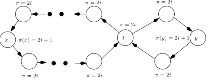
Optimal strategies for parity games (and generally for priority mean-payoff games) are under-selective. To illustrate this problem let us consider the game of Figure 6.2. x π(x) = 2i + 1 t π= 2i π= 2i π= 2i π= 2i π= 2i π= 2i π= 2i y π(y) = 2i + 1
Figure 1. The left and the right loop contain one state, x and y respec-tively, with priority 2i + 1, all the other states have priority 2i. The weight of all states is 1. The reward for x and for y is 1 and 0 for all the other states. This game is in fact a parity (B¨uchi) game, player 1 gets payoff 1 if one of the states {x, y} is visited infinitely often and 0 otherwise.
For this game all strategies of player 1 guarantee him the payment 1. Suppose however that the left loop contains 21000000 states while the right
loop only 3 states. Then, intuitively, it seems that the positional strategy choosing always the small right loop is much more advantageous for player 1 than the positional strategy choosing always the big left loop. But with the traditional definition of optimality for parity games one strategy is as good as the other.
On the other hand, Blackwell optimality clearly distinguishes both strate-gies, the discounted payoff associated with the right loop is strictly greater than the payoff for the left loop.
Let us note that under-selectiveness of simple mean-payoff games origi-nally motivated the introduction of the Blackwell’s optimality criterion [2].
6. FINAL REMARKS 23
Indeed, the infinite sequence of rewards 100, 0, 0, 0, 0, . . . gives, at the limit, the mean-payoff 0, the same as an infinite sequence of 0. However it is clear that we prefer to get once 100 even if it is followed by an infinite sequence of 0 than to get 0 all the time.
6.3 Evaluating β0.
Theorem 5.2 is purely existential and does not provide any evaluation of the constant β0appearing there. However it is not difficult to give an elementary
estimation for β0, at least for deterministic games considered in this paper.
We do not do it here since the bound for β0 obtained this way does not
seem to be particularly enlightening.
The preceding subsection discussing the meaning of the Blackwell op-timality raises the question what is the complexity of finding Blackwell optimal strategies. This question remains open. Note that if we can find efficiently Blackwell optimal strategies then we can obviously find efficiently optimal strategies for priority mean-payoff games and, in particular, for par-ity games. But the existence of a polynomial time algorithm solving parpar-ity games is a well-known open problem.
References
[1] H. Bj¨orklund, S. Sandberg, and S. Vorobyov. Memoryless determinacy of parity and mean payoff games: a simple proof. Theor. Computer Science, 310:365–378, 2004.
[2] D. Blackwell. Discrete dynamic programming. Annals of Mathematical Statistics, 33:719–726, 1962.
[3] L. de Alfaro, T. A. Henzinger, and Rupak Majumdar. Discounting the future in systems theory. In ICALP 2003, volume 2719 of LNCS, pages 1022–1037. Springer, 2003.
[4] A. Ehrenfeucht and J. Mycielski. Positional strategies for mean payoff games. Intern. J. of Game Theory, 8:109–113, 1979.
[5] E.A. Emerson and C. Jutla. Tree automata, µ-calculus and deter-minacy. In FOCS’91, pages 368–377. IEEE Computer Society Press, 1991.
[6] J. Filar and K. Vrieze. Competitive Markov Decision Processes. Springer, 1997.
[7] H. Gimbert and W. Zielonka. When can you play positionally? In Mathematical Foundations of Computer Science 2004, volume 3153 of LNCS, pages 686–697. Springer, 2004.
[8] H. Gimbert and W. Zielonka. Deterministic priority mean-payoff games as limits of discounted games. In ICALP 2006, volume 4052, part II of LNCS, pages 312–323. Springer, 2006.
[9] H. Gimbert and W. Zielonka. Limits of multi-discounted Markov de-cision processes. In LICS 2007, pages 89–98. IEEE Computer Society Press, 2007.
[10] H. Gimbert and W. Zielonka. Perfect information stochastic priority games. In ICALP 2007, volume 4596 of LNCS, pages 850–861. Springer, 2007.
[11] E. Gr¨adel, W. Thomas, and T. Wilke, editors. Automata, Logics, and Infinite Games, volume 2500 of LNCS. Springer, 2002.
[12] Y. Gurevich and L. Harrington. Trees, automata and games. In Proc. 17th Symp. on the Theory of Comp., pages 60–65. IEEE Computer Society Press, 1982.
[13] A. Hordijk and A.A. Yushkevich. Blackwell optimality. In E.A. Fein-berg and A. Schwartz, editors, Handbook of Markov Decision Processes, chapter 8. Kluwer, 2002.
[14] M. Jurdzi´nski. Deciding the winner in parity games is in UP ∩ co-UP. Information Processing Letters, 68(3):119–124, 1998.
[15] J.F. Mertens and A. Neyman. Stochastic games. International Journal of Game Theory, 10:53–56, 1981.
[16] A.W. Mostowski. Games with forbidden positions. Technical Re-port 78, Uniwersytet Gda´nski, Instytut Matematyki, 1991.
[17] A. Neyman. From Markov chains to stochastic games. In A. Neyman and S. Sorin, editors, Stochastic Games and Applications, volume 570 of NATO Science Series C, Mathematical and Physical Sciences, pages 397–415. Kluwer Academic Publishers, 2003.
[18] M. J. Osborne and A. Rubinstein. A Course in Game Theory. The MIT Press, 2002.
[19] L. S. Shapley. Stochastic games. Proceedings Nat. Acad. of Science USA, 39:1095–1100, 1953.
[20] W. Zielonka. An invitation to play. In Mathematical Foundations of Computer Science 2005, volume 3618 of LNCS, pages 58–70. Springer, 2005.
6. FINAL REMARKS 25
[21] Uri Zwick and Mike Paterson. The complexity of mean payoff games on graphs. Theor. Computer Science, 158(1-2):343–359, 1996.