Crush behavior of flanged plates under localized in-plane loadings

(1)

Crush Behavior of Flanged Plates Under Localized

In-Plane Loadings

by

Mohamed Yahiaoui

Master of Science in Mechanical Engineering Massachusetts Institute of Technology

(1988)

Mechanical Engineer

Massachusetts Institute of Technology (1992)

Submitted to the Department of Ocean Engineering in

partial fulfillment of the requirements for the degree

of

..;:-•~~Hus'rrs INSTITUrE

OF TECHNOLOGY

DOCTOR OF PHILOSOPHY

APR

1 6 1996

at the

LIBRARIES

MASSACHUSETTS INSTITUTE OF TECHNOLOGY

January, 1996

© Massachusetts Institute of Technology, 1996. All Rights Reserved.

Author ...

... ... . .

Department of Ocean Engineering

January, 1996

Certified by ... ... ... ...

Tomasz Wierzbicki, Professor of Applied Mechanics Thesis Supervisor

Accepted by ...

... .

. ...

...

ProfessA.rDo 'as Carmichael Chairman, Ocean Engineering Department Graduate Committee

(2)

Crush Behavior of Flanged Plates Under Localized In-Plane Loadings

by

Mohamed Yahiaoui

Submitted to the Department of Ocean Engineering on January 25, 1996, in partial fulfillment of the requirements for the degree of

Doctor of Philosophy

Abstract

An analytical approximation for the crushing resistance of flanged semi-circular plates subjected to localized in-plane loadings has been derived. Small-scale experiments were conducted to validate the theoretical results. The loading was applied quasi-statically by a cylindrical indenter at the symmetry line of the plate.

This work provides a consistent computational model which leads to a theoretical predic-tion of the load-deflecpredic-tion characteristics. It provides the link between the two phases of the plate response: pre-failure (in the sense of maximum load) and post-failure phases. During the pre-failure phase, the plate undergoes pre-buckling, buckling, and post-buck-ling stages. Once the point of maximum strength is reached in the post-buckpost-buck-ling stage, the post-failure phase starts. This process is characterized by rapidly falling load due to plastic folding with large strains (up to rupture strain of the material) and large rotations of plate elements. Energy methods are used to analyze the elastic pre- and post-buckling response of the plate. Ultimate strength is calculated, using the membrane yield criterion. Limit analysis, applied incrementally up to large displacements and rotations, is employed in the post-failure range.

The analytical predictions were compared to the experimental results and shown to over-estimate the peak force by about 15%. A comparison of the crushing loads in the post-fail-ure phase was also made between the analytical model and test results. The correlation is within -5% to +17% depending on the indenter's radius. Possible causes of discrepancies are commented upon and a preliminary discussion on an alternative model is presented. Finally, indentation tests of flanged rectangular plates are described. This experimental study revealed good correlation with analytical results independently developed by Choi et. al. Their model predicts loads only 5-15% higher than experimental results.

The findings of this study prove important in the understanding of the overall ability of vehicle structures, such as ships, submarines, and aircraft, to withstand local damage dur-ing accidental loads. For example, the flanged rectangular plate model characterizes the behavior in the flat bottom region of both conventional and unidirectionally stiffened dou-ble hull ships during grounding accidents. The flanged circular plate model describes the behavior in the bilge area and provides estimates of the strength of submarine bulkheads in collisions or aircraft fuselages subject to crash landings.

Thesis Supervisor: Tomasz Wierzbicki

(3)

Acknowledgments

My thanks begin with Professor Tomasz Wierzbicki, my thesis advisor. I am very grateful not only for his guidance, insight, support and financial assistance but also for the opportunity to work in the unique learning environment that he created: the Joint MIT-Industry Program on Tanker Safety.

Many thanks to Professor Frank McClintock for his expertise, time and seemingly limitless patience and for providing me with all the advice and support critical to complet-ing this degree. I am indebted to him for all of his constructive criticism.

I would also like to thank Professor Koichi Masubuchi. His comments and suggestions were very helpful towards the completion of this thesis.

I offer my most sincere gratitude to Professors Dick Yue, Kamal Youcef-Toumi, Neville Hogan, David Hardt, and David Gossard, for providing me during the rough times

with much needed financial support throughout enjoyable and rewarding teaching assistantships.

Sincere thanks are extended to the friends and colleagues, too numerous to be listed here, that have all contributed in their own distinct and subtle ways to further enhance my educational experience at MIT. My greatest appreciation to each one of you.

A very special thanks to Danielle Guichard-Ashbrook of the International Students Office for assistance and inspiration far beyond the call of duty.

For helping me navigate the sea of bureaucracy, I thank Leslie Regan of the Mechani-cal Engineering Department and Teresa Coates of the Ocean Engineering Department.

Even though thanks do not even begin to repay the debt I have accumulated, much heartfelt thanks to you, Hassiba, for your help, companionship and love which made the

(4)

difference for the completion of this thesis and kept some sort of balance in my life. I am truly thankful for her presence in my life.

Last, but not least, I wish to thank my parents, Malika and Ali, who made it all possi-ble and kept me going with their unconditional love, support and encouragements. I could not have done it without you, and best of all, I can tell you now that I have graduated: I am finally done!

(5)

List of Figures

Figure 1.1: Photograph of Damaged Ship Bilge Area ... 14

Figure 1.2: Extent of Damage... 15

Figure 2.1: Flanged Semi-Circular Plate Unit ... 35

Figure 2.2: Load-Deformation Characteristic ... ... 35

Figure 2.3: Crushed Experimental Specimen ... 36

Figure 2.4: D eform ed Specim en ... ... 37

Figure 2.5: Two-degree-of-freedom Model... 38

Figure 2.6: Displacement Field... ... ... 39

Figure 2.7: Family of Load-deflection Curves in the In-plane Elastic Range ... 40

Figure 2.8: Dimensionless Elastic In-plane Stiffness vs. Extent of Damage...41

Figure 2.9: Load-deflection Curve in the Post-buckling Range and Mode Transition...42

Figure 2.10: Determination of the Buckling Load...43

Figure 2.11: Beginning of Post-buckling Phase ... ... 44

Figure 2.12: Dimensionless Load-deflection Curve for Flanged Semi-circular Plates ..45

Figure 2.13: Yield Locus for Lower Region of Model ... 46

Figure 2.14: Yield Locus for Upper Region of Model ... ... 47

Figure 3.1: Displacement Field... ... ... 58

Figure 3.2: Load-deflection Curves for Several Values of Initial Imperfections ... 59

Figure 4.1: One-degree-of-freedom Model...79

Figure 4.2: Simplified One-degree-of-freedom Model... .... 80

Figure 4.3: Decoupling of Yield Locus -Actual and Idealized ... 81

Figure 4.4: Dimensionless Load-deflection Curves in the Post-failure Range...82

Figure 5.1: Test Specimen Geometry ... 90

Figure 5.2: Experimental Set-up ... 91

Figure 5.3: T est Fixture... ... 92

Figure 5.4: Indenter of Radius 1.5 in. ... 92

Figure 5.5: Adaptor for Small Indenters ... 93

Figure 5.6: Adaptor for Large Indenter... ... ... 94

Figure 5.7: Experimental Results for Test #1 ... ... 95

Figure 5.8: Experimental Results for Test #2 ... 96

Figure 6.1: Experimental and Theoretical Pre-failure Curves ... 104

Figure 6.2: Experimental and Theoretical Post-failure Curves ... 105

Figure 6.3: Global theoretical and Experimental Load-deflections for Test #1 ... 06

Figure 6.4: Global Theoretical and Experimental Load-deflection for Test #2 ... 107

Figure 6.5: Global Theoretical and Experimental Load-deflection for Test #3 ...108

Figure 6.6: Alternative M odel Geometry ... 109

Figure 6.7: M odified M odel... 110

Figure 6.8: In-plane Displacement Field ... 111

Figure 6.9: Out-of-plane Displacement Field ... 112

Figure 6.10: Dimensionless Elastic In-plane stiffness vs. Extent of Damage ... 113

Figure 7.1: Flanged Rectangular Plate Specimen ... 1...18

(8)

Figure 7.3: Experimental Set-up ... 120

Figure 7.4: Experimental Apparatus ... 121

Figure 7.7: Original and Modified Testing Fixture ... .... 123

Figure 7.10: Crushed Specimen of Test #1 ... 126

Figure 7.11: Crushed Specimen of Test #2... 126

Figure 7.12: Crushed Specimen of Test #3... 127

Figure A. 1: Geometric Considerations ... 152

Figure A.2: Definition of Areas used in Bending and Membrane Calculations ... 152

Figure C. 1: Geometric Considerations ... 181

Figure C.2: Tetrahedron Used in the Bending Calculation... .... 181

Figure C.3: Close-up of the Tetrahedron ... 182

Figure C.4: Left Side of the Tetrahedron...182

Figure C.5: Another Tetrahedron Used in the Bending Calculation ... 183

Figure C.6: Geometry of the Problem...184

Figure D .1: San Clem ente... ... 195

Figure D.2: Chevron Oregon I...196

Figure D.3: Chevron Oregon II... 197

Figure D .4: Paul B uck... ... 198

Figure D .5: Experim ental Set-up ... 199

Figure D.6: Instron Machine Stiffness Experiment ... .... 200

Figure D.7: Measured Initial Imperfections...201

Figure D.8: ASTM A370 Flat Tensile Specimen ... ...202

Figure D.9: Engineering Stress-Strain Curve for Specimen 1...203

Figure D. 10: Engineering Stress-Strain Curve for Specimen 2...203

Figure D. 11: Engineering Stress-Strain Curve for Specimen 3 ... 204

Figure D. 13: Engineering Stress-Strain Curve for Specimen 5 ... 205

Figure D. 15: Engineering Stress-Strain Curve for Specimen 7...206

(9)

List of Tables

Table 5.1: Test Specimen Dimensions... 85

Table D. 1: Radius-to-thickness Ratios ... 187

Table D.2: Main Features of the Laser Displacement Sensor ... 192

Table D.3: Tensile Test Specimen Properties ... 193

(10)

Chapter 1 Introduction

1.1 The Need for Study of Flanged Circular and Rectangular Plates

For years, the commercial shipbuilding industry has operated under a set of design standards which are meant to ensure the safe operation of vessels under normal operating conditions. To date, still, ship design practices do not take into account extreme loads such as large impact forces and concentrated loads due to collision and grounding accidents.

With the increased carrying capacity of tank vessels (more than 500,000 DWT for the Very Large Crude Carriers), the dangers of transporting large amounts of oil, chemicals, and other hazardous bulk cargos cannot be ignored anymore. Large oil spills and environ-mental and ecological adverse effects when grounding or collision accidents occur have become a pressing problem.

Now, the maritime industry which came under severe public scrutiny in the aftermath of the grounding of the tanker EXXON VALDEZ in Alaska's Prince William Sound, is forced to address the issue of vessel performance in grounding and collision. In the United States, this spill lead to increased government regulation through the passage of the Oil Pollution Act of 1990 (OPA 90) mandating that petroleum product cargo ships operating

(11)

in U.S. waters will be of double hull construction, or designs of equivalent protection, by January 1, 2015.

OPA 90, along with the ever increasing environment importance, triggered a tremen-dous amount of research activity in the international community. One major research con-tribution is the Joint MIT-Industry Project on Tanker Safety launched on July 1, 1992 in the Department of Ocean Engineering at the Massachusetts Institute of Technology. The overall objective of the program has been to develop extensive theoretical and experimen-tally-validated engineering knowledge in the area of structural mechanics necessary to assess the extent of grounding damage to oil tankers for a variety of hull types and ground-ing scenarios. The interested reader is refered to Wierzbicki, Yahiaoui, and Sinmao (1994) for the details of the research activities within the project.

The ability of a ship to withstand damage during grounding accidents (which trans-lates directly into tons of oil outflowing in the ocean) depends greatly on the crushing strength of the ship's hull. The crushing strength of the hull comes from a resistance to the longitudinal cutting/tearing of the bottom plating and supporting stiffeners as well as from vertical indentation into longitudinal and transverse framing. The present work addresses the initiation of local damage due to vertical indentation.

1.2 Previous Work

Consistent with the distinction between the two aspects of the damage process, described above, the publications dealing with the mechanics of ship grounding can be divided into two categories: Those studying cutting of plates by a wedge and those devoted to vertical indentation of a punch into a plate or stiffened panel.

Quasi-static and drop-hammer tests in which a rigid rounded-nose wedge was pushed into a plate along an axis parallel to the plate surface have been performed by Akita et al.

(12)

(1972), Akita and Kitamura (1972), Vaughan (1979, 1980), Woisin (1982), Jones and Jouri (1987), Goldfinch (1986), Prentice (1986), and Lu and Calladine (1990). This type of research has been proven useful in identifying some important factors which control the resistance force in grounding, including plate thickness, cut length, and ultimate stress of the material. Vaughan (1978), applied the results of the plate cutting experiment to the grounding resistance of ships, following an earlier idea by Minorsky (1959). He postu-lated that the energy absorption during the grounding process can be approximated by the total volume of damage and proportionality constants determined empirically from the data of Akita and Kitamura (1972). Recently, at MIT several aspects related to this type of research have been extensively studied from the theoretical and experimental point of view. Numerous reports were published during the period from July 1992 to July 1995 under the Joint MIT-Industry Project on Tanker Safety.

The second category of experiments in which a rigid punch was pressed into a stiff-ened plate along an axis normal to the plate surface are exemplified by the work of Ueda et al. (1978), Arita and Aoki (1985), and Ito et al. (1984, 1985, 1986). Finite element analy-ses were also performed and the two approaches were correlated with good results.

At MIT a theoretical/experimental study was initiated by Culberston-Driscoll (1992) to analytically predict local crushing of flat rectangular flanged plates. A simple model was developed in which the plastic behavior of deforming web girders was viewed as a sequence of "frozen" deformation modes where the plastic zone size was treated as a parameter. Goksoyr (1994) performed a very thorough numerical study of the elastic buckling and the plastic crushing deformation modes using the finite element code ABAQUS. Tests on local crushing of flat rectangular flanged plates were run by Yahiaoui et al. (1994). Based on the results of the numerical and experimental work, Choi et al. (1994) modified and improved the solution proposed by Culberston-Driscoll (1992). Their

(13)

new model predicting the load-deflection of a flat rectangular flanged plate subjected to local in-plane crushing loads showed values only 5-15% higher than experimental results. These results showed that a relatively simple analytical solution provides an accuracy at least equal to or surpassing the one of finite element solution.

1.3 Aim of Present Study

The objective of this work is to assess the crushing behavior of flanged semi-circular plates under localized in-plane loadings. A consistent computational model which leads to a theoretical prediction of the load-deflection characteristics is developed. The curved geometry is of great importance in the study of crushing strength of ships in the surround-ings of the bilge area (See Figs. 1.1 and 1.2). Such types of damage could occur while under way, docking, maneuvering, turning, and drifting due to loss of steering, power, etc. This work, will also find a direct application in submarines and aircraft structures. It provides an estimate of the strength of submarine bulkheads in collisions and of aircraft fuselages subject to crash landings.

Small-scale experiments are conducted to validate the theoretical results. Both semi-circular and rectangular flanged plates are tested. The results from the rectangular flanged plates tests are compared to the analytical findings independently developed by Choi et al (1994).

(14)

Figure 1.1: Photograph of Damaged Ship Bilge Area

(15)

: :::::-·:;i:r*: '· ~*:·i: :~:ii-· iiii-i... rt .. · .: ,· -:-:-·· - .I .: :-: : ii! :ia~ii~sj~·::~~: . ·::,i· ::::.-:: :::.: :I, ::,:i -:·:i:::: jl.i-.2. :cr:::·-i::z-::·:::::r:~ `:' :: :''-:'~··::'~;~:::-:::::: t 3::":: 'i: :j.:::s::"~::-:::::: :i:: :::-::.~'8'j!_ $. :~::i~ :: ::~?: ·~ _-~,;: _ i:::: ;I:-_I;:a:::::i ::-:r: · 'i::::I: I:i:::::i:i~~~~·~::::;:_j :':':"7'''"::::: "i~~i-ii Shell defection 250'm

Area of Web Frame Buckling Extent of Shell Plate Indentation

Figure 1.2: Extent of Damage

.alp~;:

(16)

Chapter 2 Circular Flanged Plates

-

Pre-failure Analysis

In this chapter, the load-deformation characteristics for a flanged semi-circular plate subject to localized in-plane loadings (Fig. 2.1) is derived. The load case considered is a quasi-static indentation by a cylindrical indenter, approximated analytically by a knife-edge loading. The diametral knife-edge of the bulkhead is fully clamped. The circumferential edge is assumed constrained by the flange to only in-plane motions.

The response of the plate consists of two phases; before and after maximum load (here called pre-failure and post-failure phases). In the pre-failure phase, the load is increasing up to the point of maximum strength; rotations are moderately large, but the strains remain small. During this phase (refer to Fig. 2.2), the plate undergoes pre-buckling (OA), buck-ling (point A), and post-buckbuck-ling (AB) stages. Near the point of membrane yielding the load is a maximum (point C), and the out-of-plane pattern of deformation becomes con-stant. This marks the beginning of the post-failure (DE) phase. This process is character-ized by rapidly falling loads due to plastic folding, with large strains (up to the rupture strain of the material) and large rotations of plate elements.

(17)

Energy methods are used to analyze the elastic pre- and post-buckling response of the plate. Ultimate strength is calculated, using the membrane yield criterion. Limit analysis (Prager, 1959), applied incrementally up to large displacements and rotations is employed in the post-failure range. This leads to a theoretical prediction of the load-deformation characteristics and provides the link between the two phases of the plate response.

In what follows, the pre-failure phase of the plate is analyzed. Each stage of the defor-mation process is quantified. Critical parameters such as the buckling load "Pcr" and the membrane yielding load "Pu" are derived. The membrane yielding load represents the force level at which the membrane yield occurs and is assumed to be the point at which the pre-failure phase ends and the post-failure phase begins. This applies to the materials and geometries in proportions comparable to those of the ship bilge area. A complete analysis of the post-failure phase is undertaken in Chapter 4.

2.1 Displacement Field

In applying energy methods (Timoshenko and Woinowsky-Krieger, 1959), one must first assume suitable displacement fields. The expressions for these fields will contain some arbitrary parameters, the magnitudes of which are found for minimum elastic strain energy or limit load.

Experiments give invaluable information regarding the deformation patterns that take place in the structure. The experimental observations are used in postulating the displace-ment field and in developing computational models.

2.1.1 Experimental Observations

Fig. 2.3, shows photographs of crushed experimental specimen. As revealed by the photographs, the deformation initially is primarily within a bounded region. As the

(18)

inden-tation process progresses, the lateral extent of the bounded region or "deformed zone" remains constant during all tests. Outside of the initial deformed zone, the plate undergoes small but increasing bending along the ridge lines 'OD' and 'OE' as depicted in Fig. 2.4. The lateral extent of the deformed zone is indicated by ý. It is considered to be an unknown of the process. The curves 'AB', 'BC', 'AC', and 'AOC' represent the bending ridge lines within the deformed zone. Details of the experimental investigation are pre-sented in Chapter 5.

2.1.2 Simplified Two-degree-of-freedom Model

Based on the above experimental observations, a simple two-degree-of-freedom

model of the circular flanged plate was developed. Fig. 2.5, shows the assumed model geometry. As indicated, the curved bending ridge lines are approximated by the straight lines 'AB', 'BC', 'AC', 'AO', and 'OC'. Also, piece-wise flat plane surfaces are used to approximate the curved areas 'ABC' and 'AOC'. Moreover, during the pre-failure range, the small amount of bending outside of the deformed zone is neglected. That is, if 1 is the boundary of the deforming zone then:

u = v = w-0 at F

where u, v, and w are the displacements in the x, y, and z directions respectively.

The deformation itself, within the constrained zone, consists of in-plane compression and out-of-plane bending. The maximum in-plane displacement is represented by uo and the maximum out-of-plane displacement by wo0. Displacement uo occurs at the point of

application of the compressive load P. When buckling occurs, it is assumed (as shown in Fig. 2.6) that the upper and lower zones within the deformed zone of the model rotate with respect to each other and deform in such a way that the out-of-plane displacement field

(19)

w (x, y) takes the form of a 'pyramid' with four lines of slope discontinuities. Out-of-plane displacement wo occurs at the junction between the upper and lower zones. At this junction, the in-plane displacement is u*. wo and u* are arbitrary parameters. Their

mag-nitudes as function of uo are determined in the next Section.

Note, as shown in Fig. 2.5, the upper zone of the deformed region (where 11 5 x 5 1 + X) extends a distance 2 laterally and a distance X transversely while the lower zone (where 0 < x5 Ti ) extends a same distance 2 laterally and a distance i1 transversely. The distances X and rl are related geometrically to ý through the radius R of the circular plate as follows:

S(~) = R-R - (2.1)

2

=

_R+

R 2(> (2.2)

Consult Appendix A. I1 on page 135 for detailed derivation of Eqs. (2.1) and (2.2).

Using all above assumptions, a particular form of the three components of the dis-placement field u (x, y) , v (x, y) , and w (x, y) are postulated. u, v, and w are the dis-placement in x, y, and z directions respectively. As shown in Appendix A.2 on page 136, the displacement field can be expressed by the following equations:

**u*(-- + )**

;for 0•x•<1

u (x,) + u*( +

x

+ ; for 5 x:rl+ (2.3)

(20)

;for 0_xirl

(2.5) ;for iix_<ri+

2.2 Strain Field

From the theory of moderately large displacements of plates, the strain-displacement relations are found to be:

1 1

• = 2 (uj

p

+ U ) + ww (2.6)

Eq. (2.6) is written in indicial notation and reduces explicitly to the following three equa-tions =_U ₂₁

w

x)

av y + =1(u +v)+ 1 w Dw Ex= 2F, x 2 1x ay

The above equations used in conjunction with the postulated displacement field (Eqs. (2.3), (2.4), and (2.5)) yields a complete description of the strain field.

Appendix A.3 on page 138 shows the detail of the calculations. The three components of the strain field ex, y , and Exy are given by:

w (x, y) = xy

-ý t

r i

+

aw

ay

(21)

1 1 2

U* +-W 2 ;for O_<xrl

1 1 21x (2.7)

u

o

+ ýu + -iWo ; for

-+x_<rl+

1 2

2 ;for O<x:5i

Ex = 2(2.9)

u* + .1 W2_o ;for rl5 xrl+

Note that the components of the strain tensor depend only on the known radius of the plate, and unknown in-plane displacements uo and u*, out-of-plane displacement wo₀, and parameter of the process ý. Keep in mind that X and rl are geometrically related to 5 through Eqs. (2.1) and (2.2).

2.3 Primary and Secondary Equilibrium Paths

In what follows, we make use of Wierzbicki and Huang (1991) and Geiger (1989) for-mulation. They determined the equilibrium path of a crushed box column by using the principal of virtual work.

However, one needs to point out as stated by McClintock and Argon (1966) that for small strains and displacements, there is an upper bond theorem for the elastic stiffness when a complete displacement field is postulated. In the present analysis, as usually done, we neglect through thickness stresses and displacements to end up with a simpler

(22)

dis-placement field to use in finding the energies. Strictly speaking this is not an upper bond, but experience has shown that such fields give good approximations.

Considering half of our model (because of symmetry) and defining -I to be the total potential energy, P the total compressive force, and Um and Ub the membrane and bending

energies respectively, we get

- (Uo, Wo) = Um (uO, WO) + Ub (uO,' w) - u0 (2.10)

The calculation of Um and Ub are carried out in Appendix A.4 on page 140. The final

result is given by the following:

Et 4 2 2 2 2

Um

2Et v2) CW- + C2u 0 + C3u*w0+ C4 * 0 +C 5 *2 + C602] (2.11) 2 (1 - V2 ) Et 2 Ub = 24( V2 ) C7WO (2.12) 24 (1 - v2 (

where E and v denote, respectively, the Young's modulus and the Poisson's ratio and t the thickness of the plate. The coefficients Ci (i = 1, ... , 7 ) all depend on geometric

parameters only, the radius R, and the unknown of the process, ý. For exact expression of the coefficients, consult Appendix A.4 on page 140.

It should be pointed out that the present model gives a good approximation of the membrane energy, but a less accurate approximation of the bending energy. This is due to the fact that we had to smooth-out the edges of the 'pyramid' in the bending energy calcu-lation because slope discontinuities are not admissible in elastic structures. Details perti-nent to the smoothening process are described in Appendix A.4 on page 140.

(23)

Making use of Eqs. (2.11) and (2.12), the total potential energy defined by Eq. (2.10) reduces to the following expression

Et [Clwo4 2(1 - v2) + C5u*2 + _C 6u 2

aH

condition 8 - a11

a

_u_o

auo

+ C₂ _{+ C}₃_u*w 0 + C4u*u0 + Et3 _Co 2 _1Pu 24 (1 - v2) - 2P u

an

+

al

_au*

u**

₊ 0 _S_8w o = 0 applied to the awo

above expression, gives rise to a system of three nonlinear algebraic equations relating P, uo , u*, and wo as follows:

al

_ Et C2WO2 2u o 2(1 -v 2) C4u* + 2C6u0 -

2=

P = 0 which reduces to and Et 2 (1 -v 2₎ 2 _{= 0}

IC3

**C4Uo+2C5u* = 0**

which reduces to = C3 2 C4 2C5 Fro 2C5&

S(u

o,

W

o

)

=

The equilibrium

S=

Et

[C22

+ C4u* (1 - v2) + 2C6u0o (2.13) and (2.14)

(24)

an

_l-_{_}

Et

_Et [4Cw_4CWo3 ₊_{2C2uoW + 2C3u.Wo]}

2Ctu3

₊ E _Et3 _CW ₀

Wo 2 (1 - v2) 12 (1 - v

2₎ ₀

which reduces to

WO[4CWO 2+1 2C UO+2 2C 3U*+C7] = (2.15)

Now, using the optimal value of the in-plane displacement u* given by Eq. (2.14) in Eqs. (2.13) and (2.15), the following system of two non-linear equations in uo and wo is

found: Et 1 -v2

[I

2C

6

C42 2C 5

Suo

+ C

2 SC ₅₄ ₀₂ 2C5 'WO (2.16) and

WO [4Ci

C3.2

_{C5 )}

`wO

2 + 2C₂ SC3 C4 C7t t C5

)

6

From Eq. (2.17), one can identify two distinct solutions for the out-of-plane displace-ment wo as function of the in-plane displacement u₀_.

The first solution,

wo = 0

for all uo, defines the in-plane elastic or primary equilibrium path.

The second one,

(25)

4C

32

2 2C

C4

7 t

2 ₌ Sor

or

2 -wo C7t2 6 4 6 32 (2.18)

defines the buckled elastic or secondary equilibrium path.

Now, one can write the final expression for the primary equilibrium path by inserting the value of w_o= 0 into Eq. (2.16) and letting P, stand for the primary equilibrium path load. And the final expression for the secondary equilibrium path by inserting Eq. (2.18) in (2.16) and letting P11 denote the secondary equilibrium path load. The final result is

given by the following two equations;

S Et C4J I 1- v 22C6 2C4- 5u 0 (2.19) 2 Et C42 P = V 2C₆ ₂

" -1 -v2

L

6 C7 C2 C2 C4

t2 2C 5 (2.20)

S 4C

(2.20)

5

(26)

1 + 1 1 1 1 _ 1, 1 1 C( + + -+ - + -a 8 3 8 3 4 • 8 3 8 3 4 -1 - Iv 2 2 22 1 1

C

()

-=

5 +I 1 1 lvT 1 1 X 1 vX C5()= ₂_2l + ₄ ₄ + _{+ 2} +₊₄ _{4 5} 1 0

C6=

2 .

C (+ + 2 +- +

7 3 3

"i

x

3

Using energy methods, we have succeeded with a simple two-degree-of-freedom model to identify, as the parameter ý changes, a family of primary and secondary equilib-rium curves given by Eqs. (2.19) and (2.20).

Now, we will make use of dimensionless parameters to get a generalized description of the process. Working from the dimensionless equations, pre-buckling, buckling, and post-buckling stages of the pre-failure phase will be quantified by tracking how the parameter

r changes.

An appropriate dimensionless parameter for the unknown of the process ý is

(2.21)

R

where R is the radius of the circular plate.

(27)

- PR P =

_D

(2.22) and - uR u = _(2.23) t2

where t is the thickness of the plate and D is the flexural rigidity of the plate defined by the following expression:

Et3

D=

12(1 -v 2₎

With the above definitions, a dimensionless form of Eq. (2.19) is given by:

-2

C

4 P, = _{12 2C}

6 -' 2C₅

and a dimensionless form of Eq. (2.20) by:

(2.24) (2 C3 C4 I2 - __ - 2 2C5

--2

4C1 C3 ₁ 5 -S2C7 _C2 U 0 _C-2

C

4 C I - C 5

The step by step derivation is shown in Appendix A.5 on page 145 along with the expressions for the parameters Ci ; (i = 1, ... , 7 ) .

PH _II- = 12 -2 C4

2C5

2C6

2C5 4

(2.25)

(28)

2.4 Pre-buckling Stage

Fig. 2.7, shows a family of load-deflection curves in the pre-buckling stage for several values of C. Clearly, there exists a value of ý for which the stiffness of the plate is mini-mum. It is this value of C that will govern the pre-buckling stage (plate remains in-plane) of the deformation process. The structure, therefore, follows the primary equilibrium path corresponding to the minimum stiffness. To determine which path it is and the correspond-ing value of C, the dimensionless stiffness of the plate as function of the parameter ý is plotted in Fig. 2.8. The lowest stiffness occurs when • = 1. Hence, the deformed zone

extents to the entire plate during the in-plane elastic phase (pre-buckling).

A limit analysis as C approaches the value 1, gives the following:

lim = 1; lim 1T = 0; lim C6 - 2

limC 4 =-1 ; lim C5 = + ; and

-2)

C4

Stiffeness of Primary Path = lim 12 2C6 - = 12 ;

C-4 1 2C 5

Finally the primary equilibrium path is described by:

P, = 12u₀ (2.26)

and

(29)

2.5 Buckling Point

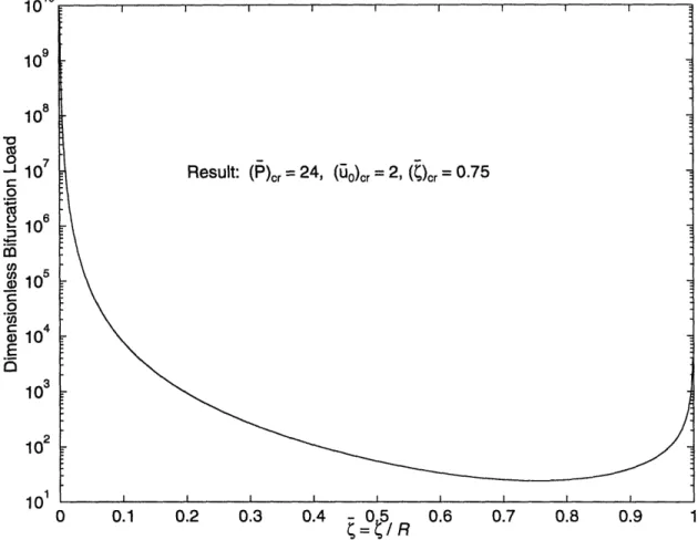
Fig. 2.9, shows the pre-buckling load-deformation curve given by Eq. (2.26) and a family of post-buckling curves for several values of • given by Eq. (2.25). The locus of the bifurcation loads as ý varies from 0 to 1 is plotted in Fig. 2.10. The lowest bifurcation load (called here Pcr) is obtained at ( = 0.75, and is assumed to characterize the onset of buckling. It represents the end of the in-plane phase (primary equilibrium path) and the beginning of the buckled phase (secondary equilibrium path).

As seen in Fig. 2.10, the buckling load Pcr is:

Pcr = 24 (2.28)

and the corresponding critical in-plane displacement (o)cr is:

(o cr = 2 (2.29)

The above results are found by first equating Eqs. (2.25) and (2.26) and solving for uo)cr as function of ý. Then, second by using this result in Eq. (2.26) and minimizing with respect to ý.

As depicted in Fig. 2.11, the onset of buckling leads to an immediate drop in axial stiffness to about 0.6 of the pre-buckling stiffness. In order to check the validity of our approximate solution, we compared our result with the exact values of 0.5 and 0.408 for rectangular plates loaded in compression by a distributed force with edges kept straight and edges free to wave, respectively (Rhodes, 1989). As seen, our approximate value compares favorably well with the exact ones given the different nature of the problem at hand.

(30)

2.6 Post-buckling Stage

Referring to Fig. 2.9, and focussing on the secondary equilibrium path given by:

PH = 12

C3 C4

2C7 c2

-2

C₅

we see, as the axial shortening increases, a further reduction in the plate stiffness. The load-deflection curve follows the envelope of a family of straight lines with various values of ý = I/R. Fig. 2.12, shows the final result for both the primary equilibrium and sec-ondary equilibrium paths.

The present model predicts that the assumed 'pyramid' shape for w (x, y) in the post-buckling stage reduces gradually in size. As the loading progresses, ý decreases continu-ously from () cr = 0.75 (onset of buckling) to ( ) u corresponding to the membrane yield of the material. Soon after the membrane yield is reached, the plate would have exhausted most of its load carrying capacity. We identify the force corresponding to the membrane yield as the ultimate strength of the plate Pu, and is assumed to characterize the end of the secondary equilibrium path.

2.7 Membrane Yield

As stated above, with increasing axial indentation, the plate material will yield. In this section, we identify the most stressed part of the material and calculate the corresponding value of (C) u. 22- _{C3 C4}

- 2

C2 2C

2 C

_{-C 2}

5

6 - - 3

2C5

_C3

L

~

4C1 -

5

(31)

Assuming that the plate yields due to membrane stresses alone, the plane stress yield condition applies (Ugural, 1981):

2 2 2

ax -a (xy + a +

3 oxy

= Y0 (2.30)

where o0 is the yield strength of the material.

At the commencement of yielding, Eq. (2.30) can be expressed in terms of the compo-nents of the strain tensor by making use of Hook's law for plane stress (Crandall and Dahl, 1959):

F

Sy

a

XY

E x - 1 --V2 (Ex + VEy) E 1- -2 (Ey + VEx) E 1+v Ex y (2.31)

The corresponding equation by inserting (2.31) in (2.30) takes the following form:

E2 (1 - v2₎ 2 (E+ve2 ) E2 + 2 (Ey + VEx) (1 -v 2) E2

-

_{2 (X + Ey)}

(1-V 2) 2 E2 2 +3 2xy = (1 +v)2 xy 2 + a3E 2ExEy 3 xy =

KE

(Ey + VEx) a₀ That is:

2 2)

Ex + }y where (2.32)

(32)

V2-V+ 1 = (1 - v2) ₂ v2 - 4v + 1

2

(1 - 2) 2 3 a3 = 2 (1 +v)

Using the expressions of u* and wo as function of uo (Eqs. (2.14) and (2.18)) in Eqs.

(2.7), (2.8), and (2.9), one can conveniently express the axial and shear strains as follows:

=

D

uo

+ D

2

S(DI)*

u04 Ey = D3u0+ D4 = ;for 0 x5rl -D2* ;for il x<r5 +X (D3*) u0+ D4* -

Exy

D

5

u

o

+ D

6 (Ds*) u0+ ; everywhere ;for 05 x5l .D₆* ;for ril<xrl+X

where the parameters Di (t) ; (i = 1, ... , 6 ) and Di* (ý) ; (i = 1, ... , 6 )

in Appendix A.6 on page 147.

Now, Eqs. (2.33), (2.34), and (2.35) in Eq. (2.32) for the case where 0 < x 5 T1 leads the following quadratic equation in uo:

Au2 + Buo + [C - 2 = 0 (2.33) (2.34) (2.35) are given where (2.36)

(33)

A = alD12 + D32) -a 2D D3 + a3D52

B = 2a1 (D1D2 + D3D4) -a2 (D1D4 + D2D3) + 2a3D5D6

C = a( D22 + D42) -a 2D2D4 +a 3D62

This result is also valid for the case where rl 5 x 5 rj + X. One need only to replace the

parameters Di (0) ; (i = 1, ..., 6 ) by their counterpart Di* (0) ; (i = 1, ..., 6 ) .

A dimensionless form of Eq. (2.36) is given in Appendix A.6 on page 147. The final result is function of the slenderness ratio parameter

3

defined by

3

=-- - and takes

the following form:

-- 2 --- - 1

Auo + Buo + C(- = 0 (2.37)

The two roots (UO)u, 1 and ( u, 2 of Eq. (2.37) define the yield locus. The corre-sponding loads plotted as function of (, delimit a yield surface (Fig. 2.13). Inside this sur-face, membrane yielding does not occur. Hence, the intersection of the secondary equilibrium path (shown in dotted lines) with the boundary of the yield locus is the point at which membrane yielding occurs. Fig. 2.14, shows the final result for the case where Trix5i+ X.

These two results are for a slenderness parameter

f

= 0.2315. This value corre-sponds to the one of the specimens used in the experimental investigation. In this example, clearly, the upper zone of the model where 11 5 x < ri + X will yield first. The correspond-ing non-dimensional ultimate force P3 and extent of the deformed zone ý are:

(34)

P = 72

(35)

KnifpE.rdop I nandino Welded Semi-Circular Bulkhead Clamped Boundary Conditions

Figure 2.1: Flanged Semi-Circular Plate Unit

F

C

Figure 2.2: Load-Deformation Characteristic

(36)

(a) Global View

(b) Close-up

Figure 2.3: Crushed Experimental Specimen

(37)

Section A-A

(38)

B YA C · a, -- ---- -- --- ~ -- -·-

--(a) Before Membrane Deformation

D

(b) After Deformation

Figure 2.5: Two-degree-of-freedom Model

p(5) Compr Tensio

SRemains

In-plane I

I

r ,I I P b I,-c -e c ,I ,, c

Is

(39)

Z. w

y, V

x, U

(40)

4ý1

6 ~'a3~_ SL~ ~: \`o ·2

(41)

C, U, C-0~_CD_C CO C, o CO 53 w L_ S_U)U, CO a_U) 0 Ci u) E, 5,

ý= IR

Figure 2.8: Dimensionless Elastic In-plane Stiffness vs. Extent of Damage

(42)

N.ý' O O · ·. q i017 ltS'iQ

ý h

(43)

,10 1l 109 108 - 107 0 2- 106 Cr S10 C 4 0 10 E 102 102 I n1 0 0.1 0.2 0.3 0.4 - 0.5 0.6 0.7

Figure 2.10: Determination of the Buckling Load

(44)

0 II ,Q. "o _0₀ -j u, U) 0 C,) c-u, O E 0 0° 2 3 4 0 1 2 3 4 5 6 _7

Dimensionless In-plane Displacement uo = uoR

Figure 2.11: Beginning of Post-buckling Phase

8 9 10

(45)

0 2 4 6 8 10 12 _14 16~

Dimensionless In-plane Displacement uo= uoR/P

Figure 2.12: Dimensionless Load-deflection Curve for Flanged Semi-circular Plates 18 20

(46)

Q

II a) 7_1₀_c o C, 0) E o•

(47)

Membrane \ Yield

-...

...

... .

I

...

.... ...

.

. ...

... ...

.

. ... ..

- 0.5

ý= R

R 0.7

Figure 2.14: Yield Locus for Upper Region of Model

I 2 100 80 40 20 -20 -40

60 n

_0.55 0.55 0.75 ` w•

(48)

L-Chapter 3

Circular Flanged Plates

-

Effect of Initial Imperfections

In the preceding chapter, the plate has been considered to be perfectly flat before load application. Due to structural imperfections and welding distortions, the plate at hand is initially imperfect. In the present chapter, we will investigate the influence of these initial imperfections on the behavior of the structure.

The analysis is carried out following the same logic as in Chapter 2. First, the displace-ment and strain fields are revisited to include the effect of the initial imperfections. Subse-quently, membrane and bending energies are derived from the strain field. Finally, making use of energy methods, the load-deflection curve is determined as function of imperfection magnitudes.

3.1 Displacement and Strain Fields

In addition to the displacement fields u (x, y) , v (x, y) , and w (x, y) established in Section 2.1 on page 17, we have an additional function w (x, y) representing the initial deviation from the perfectly flat shape. For simplicity, ýi (x, y) is assumed to be of the same form of the displacement mode w (x, y) with a maximum deflection 0vo (Fig. 3.1).

(49)

Also, imperfections are introduced only in the transverse direction. There are no imperfec-tions in the in-plane direction.

The new term describing the initial imperfection is given by

/

w (x, y) =

;for O<xr-;for rl<_xrl +1

The entire displacement field is therefore described by the following four functions:

;for O<x<5l

+4

v (x, y) = 0 for 1 x r + ;everywhere ;for 0<x5rl ;for rlix5rl + ;for Ox•'rl ;for rl !xrl +

From the theory of moderately large displacement of plates and the above postulated displacement field, one can derive the strain field with initial imperfections effect as fol-lows:

u (x,y)

=

{

w x

Wo

w (x, y) = wi (x, Y)

,(

,yt

wo 0 x y h+rlh u* . x +

uo +

rl+-

_{• ,}

.

Y)

WO

Xh

Y

+~!

xx

Ye1h

(50)

1 1

E =p 2 (ua,p+ Uj) +2 (Wa W'p - wi, iV')

Du

ax

av

, =-yy S=1

au

x'2

F

y

1

2 -(Dw)

(2

l

2 a

\y

By

+v 1(

+x 2

The detailed derivation is presented in Appendix B.1 on page 153 and the final result is:

11 + 1

211

1 1+

-2 +2

2 - 2 WO -WO) w+ wo -WO E8 = 2 W2 -2) ;for 05xjrl ;for l _5x<ri + ; everywhere ;for O<x<rl (3.3) ;for rl 5x<rl +X

We also need to introduce a curvature field with initial imperfection effect given by,

_[aX 2

•% =

ax-x

( w - iv )

Exy That is

Ex

{

(3.1) (3.2) 1 * 1

1

u* i 1(

w2

-2) + W_o - W_o

= (w- ýv), ao

(51)

3.2 Load-displacement Curve

The load-displacement curve is derived using the principal of virtual work as intro-duced in Chapter 2. The potential energy,

II,

written as a function of the membrane and bending energies is minimized to lead to a set of two nonlinear algebraic equations. The solution of these equations describes the behavior of the structure in terms of a load-dis-placement curve.

The membrane and bending energies are derived in the same manner as for the case of no initial imperfections. Using the strain field result (Eqs. (3.1), (3.2), and (3.3)) in the expressions for the membrane and bending energies, and the following expressions for the average curvatures

(K. wo-

wo

XX) avg WO 2 ; for

O

x <•1i

(lx)avg

(i,1) avg 2 W ; for T1 <x 11 + X

W0 -- WO (K)avg 2

one gets, as detailed in Appendix B.2 on page 156, the following result for the membrane and bending energies with initial imperfections:

Et

2 - 2 2 2 2 Um =

2(1-v

2) C1(O - WO) + Czuo ( 0 w o -+ C3U*•( wO - 02 + C4u*uo0 + C5 2 6 2 and Et3 Ub C7 ( o-o) 24 (1 - v2)

(52)

where Ci ; (i = 1, ..., 7 ) are as defined in Appendix B.2 on page 156.

From the above expressions, the equilibrium path for an initially imperfect plate is derived. The buckling of real (and therefore imperfect) structures is gradual. Therefore, the equilibrium path for an initially imperfect plate is now described with one smooth curve where there is no distinction between the primary and secondary equilibrium paths. In essence, the introduction of initial imperfections, w~of 0, implies that wo # 0 and therefore the secondary equilibrium path describes the entire equilibrium path. The final result is given in terms of the following two non-linear algebraic equations and is derived in Appendix B.3 on page 158. 2 Et 2 C4 PII = __ v 2 2 2CC -2 _2C₅ t2C7 C2 42C

(

2

CC

( 1

(3.4)

Uo 4C,-3 and

4C,

C3C

7

t

2 C, _ - 2 _o_6

uoo

-w -(3.5)

2C2-

C C

C52 )

(-2C

C5

Expressions (3.4) and (3.5) furnish a system of two equations with two unknowns, P and wo. Given uo and for some value of the imperfection ivo one finds wo from Eq. (3.5), then P from Eq. (3.4).

(53)

3.3 Non-dimensionalization

In what follows, we find a non-dimensional form for Eqs. (3.4) and (3.5). Making use - PR - uR

of the non-dimensional parameters = - P -, and u = , introduced in

Sec-R D t2 r

tion 2.3 on page 21, one can derive the following two dimensionless equations which describe the equilibrium path for the initially imperfect plate.

P

= 12 2C6 -- 2 C4 2C5 and uo = - U

[YJ

2C2 CS C3 C4

2 C,

C-C- 2C 2C, 1

u0

.2..

1 4C,-2-1

-] C _ 1 6 2 C, - U-3 C5 where

•

18 1

+-

+

1 - 1 C2= 2 1

+-

1 ₊₄1 1 lv

<-1

•3 22 22

.4= - X

x

(3.6)

-wo)

_U

(3.7)

(54)

C-1 C-- 1 4 I Vn.

4

-- -o

2

1 .

C

7 -3

+21

2 3

The details of the derivation are omitted because the procedure is similar to the one used in Appendix A.5 on page 145.

Now, defining two new non-dimensional parameters wo and r as follows:

- Wo wo = t and w0 r=-t

Eqs. (3.6) and (3.7) can be rewritten in the following final form:

P = 12 2C6--2

C

4 2C, u _uo- (3.8) h 2 + +·z~-= r h5

(55)

62 2 2

C5

(3.9)

Fig. 3.2, shows P vs. u0 for three different values of the initial imperfection

magni-tude parameter r (r = 1, 2, and 3 ). When constructing the load-displacement curve, the values P are found for each increment in uo by minimizing P with respect to . There-fore, each point of the curve is characterized by an in-plane displacement u0 and its

corre-sponding minimum load P with respect to . As loading progresses, decreases contin-uously until the membrane yield of the material corresponding to C is reached.

3.4 Membrane Yield

The most stressed part of the material and corresponding non-dimensional ultimate load PU are found in the same manner as for the case with no initial imperfection. First, the expressions for the axial and shear strains are conveniently expressed as follows:

ex

D,)uo +Dz (D1*) uo + CY= _D.u+D4 xy Dsuo + D6( (D₅*) uo + i-o 1 o) (D2*) 1 (D3*) u0+ (D4* 1 -(D6*) ( ;for 0 x5rl ;for rl <x5rl +X ; everywhere ;for 0 -x-5•l ;for r <5xrj5 +k U0o

-W-0

ý4c- -

I -U321

(56)

where the parameters Di(t) ; (i = 1, ... , 6) and Di* () ; (i = 1, ... , 6) remain identical to the ones derived in Appendix A.6 on page 147.

Using the above equations in the plane stress yield condition (Eq. (2.32) on page 31) yields a quadratic equation in u_o,

Auo2+B(1

_WO)

uo+[C(1WoJ(

_W0

_E

1

0 (3.10)

from which the following dimensionless form, as detailed in Appendix B.4 on page 160, is derived:

-- 2

(

r- _ •2

Auo +B(1 - uo + 1 _ = 0 (3.11)

Wo WO_o

For a given slenderness parameter ratio, = 03 , and for some value of the initial imperfection r, the ultimate load P, is found from Eqs. (3.8), (3.9), and (3.11). The meth-odology is to determine uo as function of for every increment in w. using Eq. (3.9). This result in Eq. (3.8) gives P as function of . Minimization with respect to leads to a P and uo₀for each increment wo. The found value uo is used to construct the left hand side of Eq. (3.11). Membrane yield commences at the first positive root, (wo0) , of Eq.

(3.11). Finally, from this solution ultimate load P, and corresponding ý, are found. In Fig. 3.2, the membrane yield for the special case

P

= 0.2315 is represented by an asterisk symbol '*' for the three initial imperfection magnitude parameter r=-l, 2, and 3. As an illustration of the final results, we find for r = 3 the following:

(57)

P,= 70

(Uo) = 18

(58)

(59)

-0 2 4 6 8 10 12.. 14 Dimensionless In-plane Displacement uo= uRt2

Figure 3.2: Load-deflection Curves for Several Values of Initial Imperfections

(60)

Chapter 4 Circular Flanged Plates: Post-failure Analysis

In this chapter, we develop a computational model for analysis of the plate crushing resistance in the post-failure phase. Using limit analysis, applied incrementally up to large displacements and rotations, an approximate solution for the load-deformation relation-ship is obtained. In this post-failure phase, the process is characterized by falling loads due to plastic folding, with large strains (up to the rupture strain of the material) and large

rota-tions.

4.1 One-degree-of-freedom Model

Once the ultimate strength evaluated from the membrane yield condition in Section

2.7 on page 30 is reached, the plate load carrying capacity decreases. Our

two-degree-of-freedom model developed in Section 2.1.2 on page 18 can be extended into the post-fail-ure range. This model is valid up to the point of the membrane yield. Beyond this point, the plate is subjected to further unloading, and plastic deformations spread outside of the bounded region. From experimental observations, referring to Fig. 2.4 on page 37, five hinge lines 'OD', 'OE', 'DE', 'AD', and 'CE' are activated. From this point on, the

(61)

in-plane and out-of-in-plane deformations are related through the geometry of the problem and the number of degrees of freedom is reduced to one. Fig. 4.1, shows a one-degree-of-free-dom model based on the above discussion. As indicated, the curved hinge lines are all approximated by straight ones.

Further experimental observations reveal that after a slight increase in the amount of axial deflection, the out-of-plane displacement w1 grows in much faster proportion than

w0 (w1 > w0o). To simplify the calculation, we assume that w = 0 . Under this

assump-tion, a final simplified one-degree-of-freedom model is constructed and shown in Fig. 4.2. Because of symmetry, only half of the model is considered. The notation is defined as fol-lows:

-parameter that determines the location of all hinge lines R -specimen radius

0i -rotation of the ith hinge line (i = 1, ..., 5)

Ii -length of the ith hinge line (i = 1, ..., 5)

a -angle between first and second hinge lines

0 -angle between second and fifth hinge lines y -angle between third and fourth hinge lines

8 -angle between third and fifth hinge lines

01 - projection of (a + p)

02 - projection of (y + ) P -applied force

Crush behavior of flanged plates under localized in-plane loadings

Crush Behavior of Flanged Plates Under Localized

In-Plane Loadings

by

Mohamed Yahiaoui

Submitted to the Department of Ocean Engineering in

partial fulfillment of the requirements for the degree

of

..;:-•~~Hus'rrs INSTITUrE

OF TECHNOLOGY

DOCTOR OF PHILOSOPHY

APR

1

6 1996

at the

MASSACHUSETTS INSTITUTE OF TECHNOLOGY

January, 1996

© Massachusetts Institute of Technology, 1996. All Rights Reserved.

Author ...

... ... . .

January, 1996

Accepted by ...

... .

. ...

...

Crush Behavior of Flanged Plates Under Localized In-Plane Loadings

Abstract

Acknowledgments

Table of Contents

List of Figures

List of Tables

Chapter 1

Introduction

1.1 The Need for Study of Flanged Circular and Rectangular Plates

1.2 Previous Work

1.3 Aim of Present Study

Chapter 2

Circular Flanged Plates

-

Pre-failure Analysis

2.1 Displacement Field

2

R+

u*(-- + )

;for 0•x•<1

x

2.2

Strain Field

p

w

x)

-ý t

+

ay

u

+ ýu + -iWo ; for

-+x_<rl+

2.3 Primary and Secondary Equilibrium Paths

Um

aH

a

auo

an

+

al

au*

u**

al

2=

IC3

C4Uo+2C5u* = 0

S(u

W

)

=

S=

[C22

an

Et

2Ctu3

_R+

**u*(-- + )**

_au*

**C4Uo+2C5u* = 0**

_{C5 )}

_D

_{-C 2}

_C3

_{2 (X + Ey)}