HAL Id: hal-02984996
https://hal.archives-ouvertes.fr/hal-02984996
Submitted on 1 Nov 2020
HAL is a multi-disciplinary open access
archive for the deposit and dissemination of
sci-entific research documents, whether they are
pub-lished or not. The documents may come from
teaching and research institutions in France or
abroad, or from public or private research centers.
L’archive ouverte pluridisciplinaire HAL, est
destinée au dépôt et à la diffusion de documents
scientifiques de niveau recherche, publiés ou non,
émanant des établissements d’enseignement et de
recherche français ou étrangers, des laboratoires
publics ou privés.
interaction
T Hilmi, I Minchev, T Buck, M Martig, A Quillen, G Monari, Benoit Famaey,
R de Jong, C Laporte, J Read, et al.
To cite this version:
T Hilmi, I Minchev, T Buck, M Martig, A Quillen, et al.. Fluctuations in galactic bar parameters
due to bar-spiral interaction. MNRAS, 2020, 497 (1), pp.933-955. �10.1093/mnras/staa1934�.
�hal-02984996�
MNRAS 000,1–22(2020) Preprint 1 July 2020 Compiled using MNRAS LATEX style file v3.0
Fluctuations in galactic bar parameters due to bar-spiral
interaction
T. Hilmi
1,2?, I. Minchev
1†
, T. Buck
1, M. Martig
3, A. C. Quillen
4, G. Monari
5,
B. Famaey
5, R. S. de Jong
1, C. F. P. Laporte
6, J. Read
2, J. L. Sanders
7,
M. Steinmetz
1, C. Wegg
81Leibniz Institut f¨ur Astrophysik Potsdam (AIP), An der Sternwarte 16, D-14482, Potsdam, Germany 2Astrophysics Research Group, University of Surrey, Guildford, Surrey GU2 7XH, UK
3Astrophysics Research Institute, Liverpool John Moores University, 146 Brownlow Hill, Liverpool L3 5RF, UK 4Department of Physics and Astronomy, University of Rochester, Rochester, NY 14627
5Universit´e de Strasbourg, CNRS UMR 7550, Observatoire astronomique de Strasbourg, 11 rue de l’Universit´e, 67000 Strasbourg, France 6Kavli IPMU (WPI), UTIAS, The University of Tokyo, Kashiwa, Chiba 277-8583, Japan
7Institute of Astronomy, University of Cambridge, Madingley Road, Cambridge CB3 0HA 8Universit´e Cˆote d’Azur, Observatoire de la Cˆote d’Azur, CNRS, Laboratoire Lagrange, France
Accepted 26 June 2020
ABSTRACT
We study the late-time evolution of the central regions of two Milky Way-like simu-lations of galaxies formed in a cosmological context, one hosting a fast bar and the other a slow one. We find that bar length, Rb, measurements fluctuate on a dynamical
timescale by up to 100%, depending on the spiral structure strength and measure-ment threshold. The bar amplitude oscillates by about 15%, correlating with Rb. The
Tremaine-Weinberg-method estimates of the bars’ instantaneous pattern speeds show variations around the mean of up to ∼ 20%, typically anti-correlating with the bar length and strength. Through power spectrum analyses, we establish that these bar pulsations, with a period in the range ∼ 60 − 200 Myr, result from its interaction with multiple spiral modes, which are coupled with the bar. Because of the presence of odd spiral modes, the two bar halves typically do not connect at exactly the same time to a spiral arm, and their individual lengths can be significantly offset. We estimated that in about 50% of bar measurements in Milky Way-mass external galaxies, the bar lengths of SBab type galaxies are overestimated by ∼ 15% and those of SBbc types by ∼ 55%. Consequently, bars longer than their corotation radius reported in the lit-erature, dubbed “ultra-fast bars”, may simply correspond to the largest biases. Given that the Scutum-Centaurus arm is likely connected to the near half of the Milky Way bar, recent direct measurements may be overestimating its length by 1 − 1.5 kpc, while its present pattern speed may be 5 − 10 km s−1 kpc−1smaller than its time-averaged value.
Key words: Galaxy: bulge - Galaxy: fundamental parameters - Galaxy: kinematics and dynamics.
1 INTRODUCTION
Galactic bars reside in the centres of about 2/3 of nearby
spiral galaxies, as seen in the near-infrared (e.g., Eskridge
et al. 2000). Bars are typically described by their length, strength, and pattern speed. Their length can be estimated
visually (e.g., Martin 1995), by structural decompositions
of the galaxy surface brightness (e.g.,de Jong 1996;Prieto
? E-mail: [email protected]
† E-mail: [email protected]
et al. 1997;Gadotti 2011), by locating the maximum in the
isophotal ellipticity (e.g.,Wozniak et al. 1995;Laine et al.
2002; Aguerri et al. 2009), by variations of the isophotal
position angle (e.g.,Sheth et al. 2003), or by variations of the
Fourier modes phase angle of the galaxy light distribution
(e.g.,Quillen et al. 1994). Bar lengths have been found to
correlate with galaxy parameters, such as the galaxy mass, galaxy color, the disc scale-length, and the bulge size (e.g.,
Aguerri et al. 2005;Marinova & Jogee 2007;Gadotti 2011). Early-type systems host significantly larger bars than
type ones (e.g., Elmegreen & Elmegreen 1985; Men´ endez-Delmestre et al. 2007;Aguerri et al. 2009).
The bar angular velocity (or pattern speed, Ωb or Ωp)
determines at what radii resonances occur in the disk, knowl-edge of which is necessary to understand the bar’s impact on the disk dynamics. While bar length and strength can be
directly measured from the observations, estimating Ωb in
principle requires kinematic information. To get around this, indirect methods have been developed, e.g., by identifying rings in the disk morphology with the location of the Lind-blad resonances or sign-reversal of streaming motions across
the corotation radius (CR, e.g., Buta 1986; Jeong et al.
2007). A model-independent direct measurement of Ωbusing
kinematics is the Tremaine-Weinberg method (Tremaine &
Weinberg 1984, hereafter TW). This has been applied
exten-sively to individual external galaxies (e.g.,Merrifield &
Kui-jken 1995;Aguerri et al. 2003;Meidt et al. 2009), SDSS-IV
MaNGA IFU data (Bundy et al. 2015;Guo et al. 2019), the
CALIFA survey (S´anchez et al. 2012;Aguerri et al. 2015), as
well as to the Milky Way (hereafter MW,Debattista et al.
2002;Sanders et al. 2019;Bovy et al. 2019).
Unlike in external galaxies, the MW bar is hard to ob-serve directly owing to our position in the disk plane, there-fore, indirect approaches have been used to determine its length, strength, orientation, and pattern speed (for a
re-view, see Bland-Hawthorn & Gerhard 2016). Until about
five years ago, the bar half-length was thought to be well
constrained to Rb ∼ 3.5 kpc and its pattern speed to
Ωb∼ 50 − 60 km s−1 kpc−1, based on matching
longitude-velocity (` − V ) diagrams of HI and CO gas in the inner MW (Englmaier & Gerhard 1999), the position of the
La-grangian point L4 (Binney et al. 1997), the position of the
Hercules stream in the u − v plane (Dehnen 2000;Fux 2001;
Antoja et al. 2012;Monari et al. 2017b), the Oort constant C (Minchev et al. 2007; Siebert et al. 2011; Bovy 2015), and some low-velocity moving groups in the u − v plane (Minchev et al. 2010), although lower Ωbestimates did
ex-ist (e.g., Weiner & Sellwood 1999;Rodriguez-Fernandez &
Combes 2008).
Starting withWegg et al.(2015),Sormani et al.(2015),
Li et al.(2016), andPortail et al.(2017), more recent works using different datasets and methods have suggested a signif-icantly longer bar than previously thought (∼ 5 kpc) and a pattern speed much lower than previously accepted (35 − 45
km s−1kpc−1, e.g.,Hunt & Bovy 2018;Sanders et al. 2019;
Clarke et al. 2019; Monari et al. 2019; Bovy et al. 2019).
In contrast, Anders et al. (2019) found a bar-shaped
fea-ture inclined by ∼ 40◦ with respect to the solar azimuth
and a length of ∼ 3.5 kpc in the stellar density
distribu-tion of Gaia DR2 data (Gaia Collaboration et al. 2018a) for
stars brighter than G = 18, using distances derived with the
StarHorse code (Santiago et al. 2016;Queiroz et al. 2018).
Some studies find consistency with both a slow and a fast
bar (Hattori et al. 2019;Trick et al. 2019).
To some degree, such disparity may result from the dif-ferent methods used to measure the bar length. There could be also dynamical reasons for finding different bar lengths
and pattern speeds, as we will argue in this work. Quillen
et al.(2011) noted that in their N-body simulations the bar length visibly fluctuates in R − φ density maps, resulting from the interaction with the inner disk spiral structure, as spirals connect and disconnect from the bar ends. Time
de-pendent fluctuations in bar length, strength, and pattern
speed were found in double-barred N-body models by Wu
et al.(2018), interpreted as the interaction between the two bars moving with different pattern speed.
The present work studies two hydrodynamical simula-tions of MW-like disks forming in the cosmological context, in an effort to quantify variations in bar parameters on a dynamical timescale. Implications for the MW and external galaxies are discussed.
This paper is organized as follows. In §2 we describe
our two simulations and in §3 our three methods of
bar-length measurement are introduced. In §4we quantify the
time oscillations of the bars’ lengths, amplitudes, and pat-tern speeds. Interpretation for these fluctuations is offered
in §5, where we perform power spectrum analyses relating
bar oscillation frequencies to the reconnection between bars and spiral modes of different multiplicity. A comprehensive
discussion is presented in §6, where we relate to other
nu-merical work and make predictions for both observations of external galaxies and the MW. Finally, we conclude with a
summary in §7.
2 SIMULATIONS
We consider the last 1.38 Gyr of evolution before redshift zero from two simulations in the cosmological context with disk properties close to those of the MW, e.g., both having central bars, velocity dispersion radial profiles compatible with observations, and the presence of spiral arms.
The first simulation was first presented byBuck et al.
(2018) and is out of a suite of high-resolution
hydrody-namical simulations of MW-sized galaxies from the
NIHAO-UHD project (Buck et al. 2019a, galaxy g2.79e12, hereafter
Model1). This galaxy was simulated using a modified ver-sion of the smoothed particle hydrodynamics (SPH) solver
GASOLINE2 (Wadsley et al. 2017) and star formation and
feedback are modelled following the prescriptions inStinson
et al.(2006) andStinson et al.(2013). The total stellar mass
of Model1 is 1.59 × 10¹¹ M
. The galaxy is resolved with
∼ 8.2×10⁶
star, ∼ 2.2×10⁶gas, and ∼ 5.4×10⁶dark matter
particles (Table 1 inBuck et al. 2019b), which corresponds
to a baryonic mass resolution of ∼ 3 × 10⁴ M per star
particle (∼ 9 × 10⁴ M
gas particle mass) or 265 pc force
softening. For more details on the simulation details and
galaxy properties we refer the reader toBuck et al.(2019b).
Model1 was also used to study the chemical bimodality
of disk stars (Buck 2020) and its satellite galaxies closely
fol-low the observed satellite mass function (Buck et al. 2019b).
To properly study the time evolution of the disk’s central re-gion we require closely spaced time outputs, here using snap-shots every 6.9 Myr. This ensures that the central barred region (where the period is ∼ 100 Myr) would have over a decade of complete rotations.
The second model is from a suite of 33 simulations
presented by Martig et al. (2012) (the g106 galaxy,
here-after Model2) and also studied extensively in the past (e.g.
Martig et al. 2014a,b, Kraljic et al. 2012, Minchev et al. 2013, 2014a,b, 2015, Carrillo et al. 2019). Time outputs here are separated by 4.5 Myr. The simulation is run using
a re-simulation technique first introduced in Martig et al.
Fluctuations in bar parameters
3
& Combes(2002,2003). The spatial resolution is 150 pc andthe mass resolution is 3 × 10⁵M for dark matter particles,
7.5 × 10⁴ M
for star particles present in the initial
condi-tions, and 1.4 × 10⁴ M for gas particles and star particles
formed during the simulation. Model2 has a stellar mass of
∼ 4.3 × 10¹⁰
M (within the optical radius of 25 kpc) and
a dark matter mass of ∼ 3.4 × 10¹¹ M .
Originally Model1 and Model2 have disk scale-lengths
of hd ≈ 5.6 and hd ≈ 5.1 kpc and roughly flat rotation
curves at Vc ≈ 340 and Vc ≈ 210 km s−1, respectively.
We rescaled both models’ positions and velocities in order
to match measurements for the MW: hd = 3.5 kpc and
Vc= 240 km s−1(Bland-Hawthorn & Gerhard 2016), which
affects the mass, M , of each particle according to the
rela-tion GM ∼ V2R, where G is the gravitational constant. We
chose an hdvalue near the upper limit of the
recommenda-tion byBland-Hawthorn & Gerhard(2016) so that the bar
lengths do not become too short.
2.1 Bars
After the rescaling, both Model1 and Model2 have very
similar bar lengths1 at the final time, R
b ≈ 3.05 kpc and
Rb ≈ 3.2 kpc, respectively, but arrive there by different
paths. During the period studied, Model1’s bar length de-creases monotonically by about 10% while that of Model2
increases by the same amount (see dotted-red lines in Figs.3
and 4). As may be expected, the pattern speeds change
in the opposite directions with final values of ∼ 80 and
∼ 50 km s−1 kpc−1, respectively. The bar lengths quoted
above are the “true” values, the meaning of which will be-come clear in the next sections. Typically bars are found to slow down and to grow in length with time (as in Model2) due to losing angular momentum to the disk and dark mater halo. The opposite behavior of Model1’s bar is due to gas in-fall at this particular time period, given that the simulation is unconstrained and in the cosmological context.
Having the same length but very different pattern speeds places the bar resonances at very different radii for each simulation. This makes Model1 comparable to the fastest bars found in observations, given by the ratio of the
bar’s CR radius to its length, R ≡ RCR/Rb ≈ 3.1/3.05 ≈
1.02; conversely, Model2 hosts a significantly slower bar,
with R = 5.6/3.2 ≈ 1.75 (e.g., see Table 1 by Rautiainen
et al. 2008), using final time values.
2.2 Spiral structure
The spirals of Model1 are more tightly wound and
multi-armed (see Fig. 1 in Buck et al. 2018), while for Model2
they are more open and dominated by two or four arms (see
top-right panel of Fig. 1 inMartig et al. 2014a or Fig. 1 in
Minchev et al. 2013), which signifies that they are stronger. Indeed, we measured spiral structure overdensity for Model1 typically ∼ 5 − 10% higher than the background, compared
to ∼ 15 − 25% for Model2 (see rightmost columns of Figs.1
and 2). These values are on the lower end of the 15%-60%
spiral-arm overdensity estimated byRix & Zaritsky(1995)
for 18 face-on spiral galaxies.
1 Estimated from the L
contmethod, described in §3.1.
Recent estimates of the MW spiral-arm overdensity in-clude ∼ 14% from modeling the radial velocity field of RAVE
data (Siebert et al. 2012), ∼ 26% needed to account for the
migration rate of supersolar metallicity open clusters near
the Sun (Quillen et al. 2018a), and ∼ 20% obtained from
matching the radial velocity field of stars on the upper red
giant branch from a compilation of data (Eilers et al. 2020).
These are somewhat larger than the spiral strength of our Model1 and quite consistent with our Model2.
3 MEASUREMENTS OF BAR LENGTH
Here we employ three methods to determine the bar length2
of Model1, two of which have been widely used in the
litera-ture (e.g.,Athanassoula & Misiriotis 2002;Wegg et al. 2015;
Wu et al. 2018) and a new approach introduced below. We use a cut of |z| < 1 kpc, where z is the distance from the disk midplane, but the results do not vary wildly for other reasonable values.
3.1 Drop in background-subtracted densities: Lcont
Since galactic bars feature very high stellar densities relative to the rest of the disk, the surface density along the bar major axis will start to drop approaching the bar ends, as
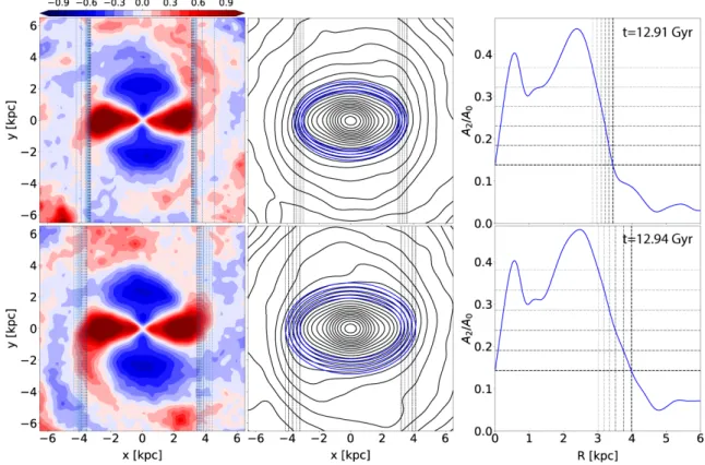
can be seen in the left column of Fig.1, which shows the
background-subtracted surface density plots for two time outputs from Model1 35 Myr apart. The density will then either fall off until it matches that of the disk (the case for the top panel) or it would be elevated if spiral structure is present nearby (as in the bottom panel).
Our new method of measuring the bar length is
some-what similar to tracing the drop of the A2/A0 Fourier
com-ponent (see §3.3), but uses instead a drop in the
background-subtracted density, considering the range between 10% and 80% above the radial mean. This range, covered in steps of 10%, is shown by the vertical dashed lines, indicating the corresponding contour levels.
An important feature of the method is that it allows one to estimate each side of the bar separately. From the
left column of Fig. 1 it is already obvious that only in a
time range of 35 Myr the bar can change length by about 10-20%, which varies depending on the choice of threshold.
3.2 Drop in disk ellipticities: Lprof
The density profiles along the bar major and minor axes
gradually become similar as radius increases.Athanassoula
& Misiriotis(2002) proposed to fit ellipses to the central den-sity region while gradually increasing radius until reaching a point where the density along the minor and semi-major axes are the same within 5%.
This method is adapted here, though with the threshold modified to use a range of ellipticities between 30% and 40% in steps of 2.5% of the difference between the bar major
and minor axes. This range covers the value used byWegg
et al.(2015) (30%) to estimate the length of the MW bar
2 Hereafter we use “bar length” to mean the length of its
Figure 1. Illustration of the three methods used to measure the bar length. For the top row we use a snapshot from Model1 at t = 12.91 Gyr and for the bottom one an output ∼ 35 Myr later. Left column: Lcont method. Face-on stellar density contours with
the azimuthally-averaged density subtracted. Vertical dashed lines mark the contour levels crossing the y-axis where the overdensity of stars has dropped by 10% to 80% from the maximum. The 50% drop is shown by the solid vertical lines. Middle column: Lprof method. Bar length is measured by fitting ellipses and measuring when the difference between the density along the semi-major
and semi-minor axis falls to below 30% to 40% of the semi-major value. Right column: Lm=2method uses the ratio of the amplitude
of the m = 2 to the m = 0 Fourier components of the stellar density, A2/A0, as a function of radius, R. The bar length is taken as the
radius where this ratio falls below a fraction of the maximum value. We here consider six thresholds from 30% to 80% of the maximum value. The larger bar estimate in the bottom row is due to its being connected to spiral arms, as seen in the left column.
in their N-body model, which was significantly higher than
the 5% ofAthanassoula & Misiriotis (2002). We also agree
with a larger threshold, as we found that a smaller one often produced abnormally large values or failed altogether.
We show the results of this bar length measurement in
the middle column in Fig. 1 over the stellar density
con-tours. As in the left column, the Lprof method measures a
longer bar for the bottom row time output by about a similar amount.
3.3 Fourier analysis of the central disk: Lm=2
An estimate of bar length can also be obtained by taking the Fourier transform over all disk azimuths. This can find the numbers, strengths, and multiplicities of non-axisymmetric
modes (Masset & Tagger 1997;Meidt et al. 2008; Quillen
et al. 2011). For each disk component being analysed, the fol-lowing coefficients of the Fourier series are first determined:
am(R) = 1 π Z 2π 0 ρ(R, θ) cos(mθ) dθ bm(R) = 1 π Z 2π 0 ρ(R, θ) sin(mθ) dθ (1)
Here, m is the azimuthal wavenumber and ρ(R, θ) is the mass density at a specific spatial bin. We estimate
Am with respect to the axisymmetric component A0, as
√
a2
m+ b2m/A0 (see, e.g.,Athanassoula & Misiriotis 2002).
Any galactic bar, which would have rotational symme-try of order two will, therefore, be highlighted in the m = 2 Fourier component, along with any 2-armed spiral structure. This allows the bar strength to be seen as a function of
ra-dius in the rightmost column in Fig.1, using 300 pc radial
and 10◦ azimuthal bins. The bar length is estimated from
the radius at which A2/A0 drops below some percentage of
the maximum strength in the range 30% to 80%, in steps of 10%. Measuring bar lengths of individual sides could then be done by reflecting one half of the disk onto the other side prior to performing the analyses. As in the previous two
methods, it is clear from the right column of Fig.1that the
bar length measured at the second time output is longer by 10%-20%, depending on the threshold used.
For our choice of thresholds, the three methods agree quite well in the ranges of bar length they measure for Model1, however, this is not going to be the case for Model2.
As will become clear from Fig.3, the top row of Fig.1shows
Fluctuations in bar parameters
5
Figure 2. As Fig.1, but for Model2. We have chosen three snapshots to highlight some typical cases. Top row: At t = 13.49 Myr, the bar is relatively well separated from spiral arms, as seen in the background-subtracted density, and the Lcontmeasured length lies in the
range ∼ 2.8 − 3.5 kpc, depending on the threshold used. This range changes to ∼ 4 − 4.2 kpc for Lprofand ∼ 1.6 − 3.2 kpc for Lm=2, i.e.,
the three methods are much less consistent than for Model1. We tend to trust the Lcontmethod more than the other two, since we can
clearly see the bar morphology and orientation with the spiral structure for each bar half. Middle row: At a time output ∼ 270 Myr later, the bar is measured to be 25-50% longer, with artifacts due to connected spiral arms clearly seen in the left panel, but not in in the total density contours in the middle or the azimuthally averaged A2/A0 variation with radius in the right panel. Bottom row: At
a time output ∼ 170 Myr earlier than in the top row, the bar is overestimated by almost a factor of two by Lcont and by ∼ 38% by
Lprof. This problem is evident from the overdensity discontinuity in the right bar half of the Lcont measurement, but is not clear from
the other two methods. In both the second and third rows the bar is connected to the spiral structure. As for Model1, we take the Lcont
measurement with threshold of 50% to be the “true” bar length at t = 13.49 Gyr, R ≈ 3.1 kpc.
argue that this then represents the “true” bar length, while
the larger bar measurement in the bottom row of Fig.1 is
caused by connecting spiral arms (this is much more
ob-vious for Model2, see §3.4). We, therefore, take the “true”
bar length at t = 12.91 Gyr to be Lcont with threshold of
50%, which corresponds to Rb ≈ 3.25 kpc. Note that this
changes monotonically with time owing to the bar’s secular
evolution, as seen in Fig.3.
3.4 Model2 bar length measurements
In Fig.2we present the three bar length measurements
ap-plied to Model2, as done for Model1 in Fig.1. We have
cho-sen three snapshots to highlight some typical cases, since this galaxy shows more complex variations than Model1. In the
top row, Lcontshows that the bar is relatively well separated
from spiral arms and the measured length is 2.8-3.5 kpc, de-pending on the drop. The left bar half is about 10% longer
owing to a connected spiral, as evident from the disturbed highest density contour.
The Lprof measurement is systematically larger, around
4 kpc. Conversely, Lm=2 varies between about 1.6 and 3.2
kpc. Note the strong disagreement among the different bar estimates compared to Model1, although the same thresh-olds were used for each model. We conclude that the “true” bar length is given by the bar side along the positive x−axis
of Lcont, as the disturbance seen in the left half must be
caused by a spiral arm. As for Model1, we take the “true”
bar length at this time to be the Lcont value with threshold
of 50%, which corresponds to Rb ≈ 3.1 kpc. We note that
this varies monotonically with time due to the bar’s secular
evolution, which can be seen in Fig.4.
The second row of Fig.2shows a case ∼ 270 Myr later,
where the bar is measured to be 25%-50% longer by all three methods. Finally, the third row shows a time output ∼ 170 Myr earlier than in the top row, where the bar is
found to be larger by almost a factor of two with the Lcont
and by ∼ 38% with Lprof methods. For Lm=2 the m = 2
amplitude does not drop below 50% for the radial range of 6 kpc shown in the plot. This means that this method
would measure a length > 6 kpc for larger drops in A2/A0,
which would clearly be incorrect. Comparing A2/A0between
the two models reveals also that Model2 has a significantly stronger spiral arm overdensity.
From the Lcont plot in the bottom row of Fig. 2 it is
obvious that the spiral arm orientation is such that it adds
to the bar length, however, in the case of Lprof even a visual
inspection would not catch this problem, since the density variations along the bar major axis are not seen in the to-tal density, shown as the contours in the middle column.
Athanassoula & Misiriotis (2002) warned about using the latter method blindly, as in certain cases there may not be a steep drop. Here, however, we do see a steep drop for the
Lprofmethod (in the middle row the 5 thresholds are on top
of each other), yet from the Lcont measurement we clearly
see that the Model2 bar is not longer than ∼ 3 kpc. We at-tribute this discrepancy to the stronger spiral arms in this hydrodynamical simulation as opposed to the dissipationless
N-body runs byAthanassoula & Misiriotis(2002) and other
works.
Looking only at the Lprof measurement (middle column
of Fig.2) one could conclude that the bar is much larger in
the bottom panel, however, both the Lcont and Lm=2 plots
argue against this. It is clear from the Lcont plot that the
extension of the bar, especially of its right side, comes from
the strong spiral arms attached to it. Using only the Lprof
method can, therefore, lead to erroneous results, as a ran-domly selected time output may correspond to a time when the bar and spiral structure are connected. Note that when
spiral arms are stronger (as in our Model2), Lprof tends to
overestimate the bar size even when the bar is as best as
pos-sible separated from spiral arms, as in the top row of Fig.2.
This conclusion is in agreement with the results ofPetersen
et al.(2019), who showed that the bar length measured from
the extent of the x1 orbits (true length) is at or below the
minimum of their ellipse-fit-derived length (similar to our
Lprof) in their N-body simulations (see their Fig. 10).
4 TIME OSCILLATIONS OF BAR
PARAMETERS
4.1 Mean bar length
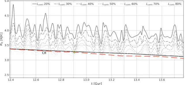
In Fig. 3we plot the bar length time evolution, Rb(t), for
Model1, using the Lcont method described in §3. Variations
with a well-defined period are seen over these last 1.38 Gyr of quiescent disk evolution, which is also true for the other two
methods (see Figs.A1andA2). The amplitude is typically
0.3 kpc (or ∼ 10%), decreasing (increasing) for thresholds that measure a shorter (longer) bar for all three methods. Note however that, as discussed below, the deviations from the “true” bar length are double that, or ∼ 20%, since the “true” bar length is given by the minimum of the time
vari-ations.
We see in Fig. 3 that the time variations for smaller
density drops have a period of Tlong≈ 125 Myr (gray
short-dashed curves), from counting 11 peaks in the period of 1.38 Gyr. As the drop increases to 50%-40% and beyond, a doubling in the frequency is seen resulting in a period of Tshort∼ Tlong/2. The more frequent oscillations appear as
we enter the disk and encounter different spiral modes of
var-ious multiplicity (as will be detailed in §5.1 below). These
are not seen from the Lprof measurement in Fig.A1, except
possibly for the 30% threshold, which may be because fitting an ellipse averages strongly over the density variation. The
Lm=2 method (Fig.A2), on the other hand, matches quite
well the Lcont variations with time, including the transition
from the lower to higher frequency with increasing density drop, for the most part.
To get the “true” bar length as a function of time we
interpolate over the minimum values measured by the Lcont
method (corresponding to when the bar and spirals are not
connected). The small green circle in Fig.3marks the time
output used in the top row of Fig.1, which corresponds to a
local minimum. Upon inspection of all measurement
meth-ods in Fig.1, we choose the Lcont threshold of 50% to refer
to as the “true” bar length at this time (Rb≈ 3.25 kpc). The
red-dashed line shows the approximate position of the min-ima for this threshold at different times, which we argued in
§3.4correspond to the true bar length. The bar is seen to
decrease with time from Rb≈ 3.35 kpc to Rb≈ 3.05 kpc in
the period of time we consider (red-dashed line in Fig.3).
The monotonic change is accompanied by an increase in
pat-tern speed (see Fig.10), such that the bar CR radius follows
closely its length. To see this, we overlaid the evolution of the mean CR radius (solid black curve marked by “CR” ), estimated form the m = 2 Fourier component in power
spec-trograms (see §5.1).
In the case of Model2, the measured bar extent (Figs.4
and A3) appears to vary much more with time than for
Model1, although the true bar length is shorter for most of
the time - compare dotted-red lines in Figs.3 and 4. The
Lcont bar length measurement shown in Fig.4varies more
erratically with time compared to Model1, as already
ex-pected from Fig.2. The period is also less regular than for
Model1 and longer overall, because of the slower bar. The small green circle marks the time output used in the top
row of Fig. 2, which corresponds to a local minimum. As
for Model1, we use Lcont with a threshold of 50% to get the
“true” bar length at this time, finding Rb ≈ 3.1 kpc. The
min-Fluctuations in bar parameters
7
CR
Figure 3. Variations with time of the Lcontbar length measurement for Model1 (see Fig.1). Light smoothing is applied. Different curves
show different threshold values in density between 20% and 80%, as indicated on top. Smooth variations with a period Tlong≈ 125 Myr are
seen for the smaller threshold values, however, additional peaks appear for the largest three thresholds with Tshort≈ Tlong/2. The green
circle marks the time output used in the top row of Fig.1, which corresponds to a local minimum. Upon inspection of all measurement methods in Fig.1, we choose the Lcont threshold of 50% to refer to as the “true” bar length at this time (Rb≈ 3.25 kpc). To get the
true bar length as a function of time we interpolate over the minimum values for the same threshold (red-dashed line), corresponding to when the bar and spirals are not connected. The bar is clearly seen to get shorter with time, starting with Rb≈ 3.35 kpc and ending up
with Rb≈ 3.05 kpc in the period of time we consider. The decrease in bar length with time is accompanied by an increase in pattern
speed (see Fig.10), such that the CR radius follows closely the bar’s length. To see this, we overlaid the evolution of the mean CR radius (solid black curve marked by “CR” ), estimated form the m = 2 Fourier component in power spectrograms (see §5.1).
CR
Figure 4. As Fig.3, but for Model2. The Lcont bar length measurement varies more erratically with time compared to Model1, as
already expected from Fig.2. The period is also less regular than for Model1 and we find a longer period overall, due to the slower bar here. The green circle marks the time output used in the top row of Fig.2, which corresponds to a local minimum. As for Model1, we use Lcont with a threshold of 50% to get the “true” bar length at this time, finding Rb ≈ 3.1 kpc. The red-dashed line results from
interpolating over such minima, which then gives the secular evolution of the true bar length. Opposite to Model1, the bar size increases with time from Rb≈ 2.9 kpc to Rb≈ 3.2 kpc in the period of time we consider. The time evolution of the CR radius is shown by the
solid-black line, found to be at a much larger radius than the bar length, compared to Model1. This is because of the lower bar pattern speed for Model2 (see Figs.10and12).
ima, which then gives the secular evolution of the true bar length. Opposite to Model1, this bar grows larger with time
from Rb ≈ 2.9 kpc to Rb ≈ 3.2 kpc in the period of time
we consider. The time evolution of the CR radius is shown by the solid-black line and is found to be at a much larger radius than the bar length, because of the bar’s low pattern
speed, compared to Model1 (see Figs.10and12).
The amplitude of oscillations in Fig.4is up to 1.5 kpc,
which corresponds to ∼ 100% overestimation, since the bar’s
true length is given by the minima. Fig.A3shows that Lprof
overestimates the bar length for all thresholds, while we found that the different methods agreed well for Model1. Unlike in Model1, using larger thresholds does not result in significantly shorter bar estimates, especially near the min-ima, which are ∼ 1 kpc above the true bar length determined
in Fig.4. We attribute this discrepancy to the stronger spiral
structure of Model2.
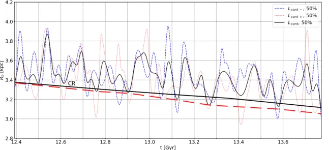
4.2 Individual bar halves
Since we would like to link our results to the MW bar, for which our current knowledge is limited to its near end, we also examined each bar half separately. This could be
achieved naturally from the Lcont method. For the other
two methods we reflected the disk density containing the bar side under consideration along the bar minor axis (i.e.,
in the case of Lprof, across the line x = 0 in the middle row
of Fig.1), after which we applied the method as before. To
make sure we did not measure different lengths for different bar halves just because our disk was not centered correctly we did a number of tests. The disk was centered by
subtract-ing the centroid of a cylinder of radius rcand height zc. We
experimented with rcand zcvalues ranging from 2 to 6 kpc
and from 0.1 to 1 kpc, respectively, finding that our results were minimally affected.
Figs. 5,A4, andA5 show the time variations in
indi-vidual bar halves (blue-dashed and red-dotted curves) for Model1 for each of the three measurement methods. For all three methods individual bar halves have larger length fluc-tuations (sometimes by a factor of two) than the mean bar length variations shown by the black curves. The length can be seen to vary by ∼ 1 kpc for Model1. As expected, a peak in the length of one side of the bar does not necessarily cor-respond to a peak in the other - these are often completely offset, i.e., a maximum length measured for one side corre-sponds to a minimum for the other (e.g., at t ≈ 12.78 Gyr
in Fig.5). It should be noted that the mean bar half-length
is not the mean of the individual sides estimated here,
ex-cept for the Lcont method. The other two methods measure
the total bar length as described in §3.2and §3.3and then
divide in half.
Fig.6shows the variation of individual bar halves for
Model2. Here we used the Lprof method, since Lcont shows
abrupt changed on a short timescale (as seen in Fig.4).
Sim-ilarly to Model1, there is no apparent correlation between
the two half-length fluctuations (seeA4) and often a peak in
the length of one bar-half corresponds to a minimum for the other. Larger maxima and minima are reached than those seen in the mean bar length measurement, but not to the extent found for Model1.
4.3 Bar amplitude
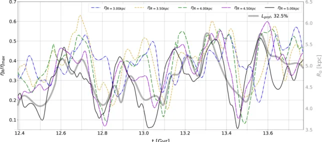
To find out if the bar length fluctuations are accompanied
by variations in the bar strength, in Fig. 7 we show the
Model1 bar amplitude at five different distances from the disk center along the bar major axis, divided by the
maxi-mum, ηR/ηmax, as indicated, where η ≡ A2/A0and ηmaxis
the maximum as a function of radius. As in Fig.1, these are
estimated from the the m = 2 Fourier mode, A2/A0, where
A0 is the axisymmetric component.
Very similar time variations appear for all radii, with
typical amplitude changes in ηR/ηmax of ∼ 0.2, except for
the innermost radius considered. The thick solid-gray curve
in Fig. 7 represents the mean bar half-length variations
(black curve from Fig.5), which can be seen to agree very
well with the amplitude fluctuations, including the short and long periods.
The fluctuations seen in the bar amplitude at fixed radii
(Fig.7) are more similar to the bar length time variations
than the ηmax, which can vary with radius (see Fig. A6).
This can generally be seen for Model2 as well in Fig.8. One
key difference between the two simulations is the fact that for Model1 all radii peak at nearly the same time, while in Model2 they are delayed with the lowest radius of 3 kpc al-ways peaking last. Such a pattern suggests a spiral arm
con-tribution. Indeed, we established in §3.4that the Model2 bar
true length is about 3 kpc, therefore the region examined in
Fig.8lies at or outside the true bar, yet in the regime where
our three measurement methods detect a bar. The solid-gray
curve in Fig.7shows the bar length time variations, seen to
follow the overall trend in ηR/ηmax, in best agreement with
the two outermost radii.
4.4 Bar pattern speed
We estimated the instantaneous bar pattern speed using the
modified TW method bySanders et al.(2019), who applied
it to both MW data and N-body simulations. The top-left
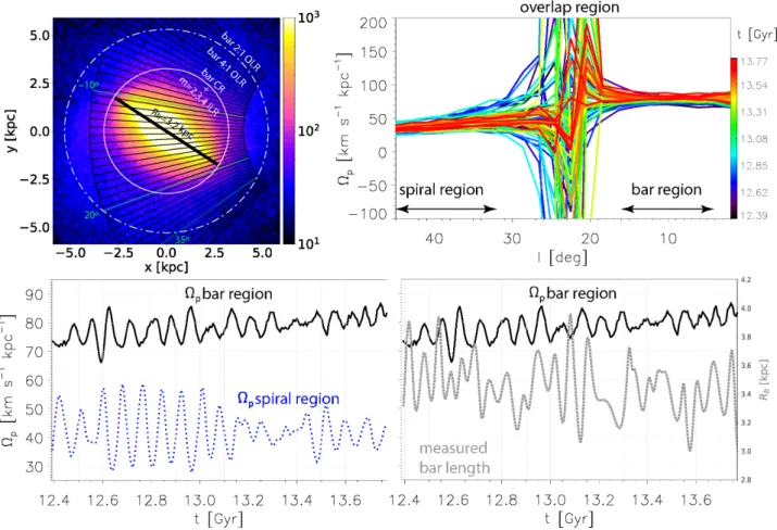
panel of Fig.9shows the configuration we used to measure
Ωp, over the stellar density of Model1. As done bySanders
et al. (2019), we assumed a bar angle of 33◦, a Galactic
latitude range |b| < 5◦, and a solar Galactocentric distance
of R0 = 8.12 kpc. The rotation is clockwise. Estimates are
done in bins of Galactic longitude dl = 2◦in the radial range
indicated by the two arches centered on the Sun (at distances of 4.12 and 8.12 kpc), which is sitting at (x, y) = (8.12, 0). The straight black line over the bar has a half-length of
3.2 kpc, which corresponds to l ∼ 17◦for our bar angle. The
bar angle is kept the same at each time output. The white circles show the bar time-median CR, 4:1 OLR, and 2:1 OLR
at RCR = 3.25, R4:1OLR = 4.2, and R2:1OLR = 5.3 kpc,
respectively. The bar CR radius coincides with the 2:1 ILR of a 2-armed, the 4:1 ILR of a 4-armed spiral, and the 3:1 ILR of a 3-armed spiral, estimated from power spectrograms
(see §5.1.1and Fig.11below).
The top-right panel of Fig.9 shows the estimated Ωp
variation with Galactic longitude, l, covering the near bar half. The color-coded curves correspond to different times,
as indicated in the colorbar. The strong divergence at 18◦.
l . 28◦ is caused by the bar-to-spiral transition, happening
between the bar CR and 4:1 OLR. To make sense of the pattern speed estimates at different longitudes (and thus,
Fluctuations in bar parameters
9
CR
Figure 5. Time variations in individual bar-half lengths for Model1, using the Lcontmethod. Lcont−and Lcont+correspond to the left
and right bar halves, respectively, as seen in Fig.1. A density threshold of 50% is used. The mean bar half-length variation with time is shown by the black curve. Significantly larger fluctuations are found for the individual halves. Individual bar halves peak in length at different times, alternating between smaller and larger maxima. We relate this to the spiral structure’s departure from bisymmetry, i.e., the bar ends do not connect to a spiral arm at the same time. The mean CR radius is shown by the black line, marked by “CR’, while the red-dashed line indicates the “true” bar length.
Figure 6. Model2 bar half-length variation with time for the mean and individual ends, using the Lprof method. The blue-dashed and
red-dotted lines show the left and right halves, respectively, for a bar fixed along the x−axis as in Fig.2. Note that the true bar length is ∼ 3 − 3.2 kpc (see Fig.4), thus, it lies outside the range of this figure. A variation of more than 40% is seen for this method and threshold, however, the overestimate from the true bar length is ∼ 90%, considering Rb≈ 5.7 kpc found around 13 Gyr. We argue that this results
from the bar-spiral structure overlap at the bar ends. The mean bar CR radius estimated from the m = 2 Fourier component of power spectrograms (see §5.1) is shown by the black line, marked with “CR’. Note that the bar’s instantaneous pattern speed fluctuates between ∼ 40 and ∼ 65 km s−1kpc−1(see Fig.10), resulting in CR radius fluctuations in the range ∼ 3.8 < R
CR< 6.4 kpc. It is remarkable
that even this very slow bar can appear “ultra-fast” for a small fraction of the time.
different distances from the Galactic center), we selected a bar-dominated and a spiral-dominated regions safely away from the transition region, as indicated by the double-arrows
in the top-right panel of Fig.9. In the bottom-left panel we
plot Ωp(t) for the “spiral region” (dotted-blue curve) and
“bar region” (solid-black curve) obtained by averaging over the longitude ranges indicated in the upper-right panel. A
very good anti-correlation is seen, which is remarkable as
these regions are separated by ∼ 16◦ in l (> 1.5 kpc along
the bar major axis). This is indicative of a bar-spiral mode
coupling (Tagger et al. 1987;Quillen et al. 2011;Minchev &
Famaey 2010;Petersen et al. 2019).
In the bottom-right panel of Fig.9we juxtaposed Ωp(t)
posi-Figure 7. Bar amplitude for Model1 at five different distances from the disk center along the bar major axis, divided by the maximum, ηR/ηmax, as indicated. Very similar time variations appear for all radii, with typical amplitude changes in ηR/ηmaxof ∼ 0.2, except for
the innermost radial bin. The thick solid-gray curve indicates the mean bar half-length variations (black curve from Fig.5), showing a very good agreement with the amplitude fluctuations. Note that as the bar decreases in length, so does its amplitude.
Figure 8. As Fig.7, but for Model2. The solid-gray thick curve indicates the mean bar half-length variations (black curve from Fig.6), showing an overall good agreement with the amplitude fluctuations. Since the true bar length is ∼ 3 kpc, the outermost three radial bins for which ηR was estimated correspond to the spiral arms, as evident from the systematic time offset among different curves.
tive longitude half (blue-dashed curve in Fig.A4). The Ωp(t)
period in both bar and spiral regions is very well defined at
∼ 80 Myr, which lies between the Tlong ≈ 125 Myr and
Tshort ≈ Tlong/2 periods of the measured bar length
varia-tion in Fig. 3. We relate these frequencies to the coupling
between the bar and spiral modes of different multiplicity
using power spectrum analyses in §5.1.1.
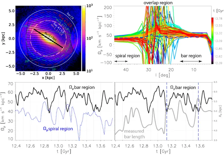
Fig. 10 is the same as Fig. 9 but for Model2. In the
top-left panel, the black line has a half-length of 3.1 kpc, in-dicating the time-median bar length. The white circles show
the bar’s time-median CR and 4:1 ILR at RCR= 5.25 and
RILR = 3.2 kpc, respectively. The orange, green, and red
circles indicate the positions of the 2:1 ILR of a 2-armed, the 3:1 ILR of a 3-armed, and the 4:1 ILR of a 4-armed spi-ral mode, respectively, estimated from power spectrograms
(see Fig.12). A ring in the stellar density is seen just outside
the bar 4:1 ILR.
As for Model1, a strong divergence in Ωp is seen in
the transition between the bar and spiral regions (top-right
panel of Fig.10), but with a wider range, 17 . l . 33,
be-cause of the stronger spiral arms. The decline of Ωpat l < 6◦
is possibly related to the perpendicular x2 orbits starting
to dominate over the bar-supporting x1 orbits. The
blue-dashed curve shows t = 13.57 Gyr, when Ωp is relatively
constant out to l = 45◦. This also corresponds to a
max-imum in the measured bar length (rightmost blue-dashed vertical in bottom-right panel).
The bottom-left panel of Fig.10shows Ωp(t) in the
“spi-ral region” (dotted-blue curve) and “bar region” (solid-black curve) obtained by averaging over the longitude ranges in the upper-right panel. A very good mirror symmetry across
Fluctuations in bar parameters
11
Figure 9. Tremaine-Weinberg method applied to Model1 as in the MW, assuming a bar angle of 33◦. Top left: Face-on view of the disk stellar density at the final time. Estimates are done in bins of Galactic longitude, dl = 2◦, in the indicated radial range (black arches) and |b| < 5◦. The Sun is at (x, y) = (8.12, 0) and the black line over the bar has a half-length of 3.2 kpc, which corresponds to the time-median Rbvalue extracted from Fig.3. The white circles show the bar’s time-median CR, 4:1 OLR, and 2:1 OLR at RCR= 3.25,
R4:1OLR= 4.2, and R2:1OLR= 5.3 kpc, respectively. The bar’s CR radius coincides with the 2:1 ILR of the 2-armed, the 4:1 ILR of a
4-armed, and a 3:1 ILR of a 3-armed spiral, as estimated from Fig.11(see §5.1.4). Top right: Estimated Ωpvariation with l for the near
bar half; color-coded curves correspond to different times, as seen in the color bar. The bar ends just inside ∼ 20◦for our bar angle. The
strong divergence at 18 . l . 28 is caused by the bar-to-spiral transition, which happens between the bar’s CR and 4:1 OLR. Bottom left: Ωp(t) in the “spiral region” (dotted-blue curve) and “bar region” (solid-black curve) obtained by averaging over the longitude ranges
indicated in the upper-right panel. The remarkable anti-correlation seen is indicative of bar-spiral mode coupling. Bottom right: Ωp(t)
in the “bar region” juxtaposed with the Lprof measurement of the corresponding bar half. The Ωp(t) period for both bar and spiral
regions is very well defined at ∼ 80 Myr, which lies between the Tlong ≈ 125 Myr and Tshort≈ Tlong/2 periods of the measured bar
length variation in Fig.3.
the line Ωb ≈ 45 is seen for most peaks, which again we
point out as remarkable (as in Model1), since these regions
are separated by ∼ 24◦(∼ 2.7 kpc along the bar major axis).
The fractional amplitude of oscillations is significantly larger than for Model1.
In the bottom-right panel of Fig.10we compare Ωp(t)
in the “bar region” to the measured bar length for the
pos-itive longitude bar half (dotted-gray curve, as in Fig.6). A
relatively good anti-correlation can be seen also here (ex-cept around 12.6 and 13.3 Gyr), with longer bar
measure-ment corresponding to slower Ωp. The blue-dashed
verti-cal lines indicate possible configurations for the MW, where
the bar appears long (∼ 5.3 − 5.7 kpc) and slow (Ωp ∼
40 km s−1kpc−1). Note, however, that the average bar
pat-tern speed is ∼ 50 km s−1kpc−1with variations around the
mean of ∼ 20%, and the true bar length is ∼ 3.1 kpc.
The variations of about 20 km s−1 kpc−1seen in the
bar region, or Ωp≈ 50 ± 10 km s−1 kpc−1, correspond to a
fluctuation around the mean of ∼ 20%. In addition to four major peaks, one can also see smaller variations on the order
of 60 Myr, many of which are also seen in the measured Rb(t)
(see bottom-right panel of Fig.10). We relate these periods
of Ωp(t) and Rb(t) to the interaction between the bar and
spiral modes, using power spectrum analyses in §5.1.3.
More discussion on Fig.10is presented in §5and
rela-tion to the MW bar is made in §6.4.
5 EVIDENCE FOR BAR-SPIRAL ARM
INTERACTION
Since bars typically rotate faster than the spiral structure, there will be times when the two components overlap
spa-tially. As discussed byComparetta & Quillen (2012), this
can be thought of as a constructive interference between
Figure 10. As Fig.9, but for Model2. The black line has a half-length of 3.1 kpc, indicating the time-median bar length. The white circles show the bar’s time-median CR and 4:1 ILR at RCR= 5.25 and R4:1ILR= 3.2 kpc, respectively. The orange, green, and red
circles show the positions of the 2:1 ILR of a 2-armed, the 3:1 ILR of a 3-armed, and the 4:1 ILR of a 4-armed spiral mode, estimated from power spectrograms (see §5.1.4). A ring in the stellar density is seen just outside the bar 4:1 ILR. Top right: Estimated Ωpvariation
with l for the near bar half; color-coded curves correspond to different times, as seen in the color bar. The bar ends just inside ∼ 20◦. As for Model1, a strong divergence in Ωpis seen in the transition between bar and spiral regions, with a wider range this time, 17 . l . 33,
due to the stronger spirals. The decline of Ωp at l < 6◦is possibly related to the perpendicular x2orbits starting to dominate over the
bar-supporting x1 orbits. The blue-dashed curve shows a case (t = 13.57 Gyr), when Ωpis relatively constant out to l = 45◦; this also
corresponds to a maximum in the measured bar length (rightmost blue-dashed vertical in bottom-right panel). Bottom left: Ωp(t) in
the “spiral region” (dotted-blue curve) and “bar region” (solid-black curve) obtained by averaging over the longitude ranges in the upper-right panel. A very good anti-correlation is seen, although not as perfect as for Model1, however, the amplitudes are significantly larger. Bottom right: Ωp(t) in the “bar region” is compared with the measured bar length for the positive longitude half (dotted-gray curve,
as in Fig.6). A relatively good anti-correlation can be seen also here (except around 12.6 and 13.3 Gyr), with longer bar measurement corresponding to slower Ωp. The blue-dashed vertical lines indicate possible configurations for the MW, where the bar appears long
(∼ 5.3 − 5.7 kpc) and slow (Ωp∼ 40 km s−1 kpc−1). Note, however, that the average bar pattern speed is ∼ 50 km s−1 kpc−1with
variations around the mean of ∼ 20%, and the true bar length is ∼ 3.1 kpc.
density plots the bar seemed to increase in length when con-nected to the spiral. It is important to consider that spiral structure is never perfectly symmetric in unconstrained sim-ulations, meaning that even 2- or 4-armed spirals will not necessarily connect to the two bar ends at the same time. This is because the density that the bar sees is a combi-nation of the different modes present in the system, which may include m = 1 and m = 3 components, as frequently
seen in simulations (e.g.,Quillen et al. 2011;Minchev et al.
2012). This can explain why the bar does not grow in length
simultaneously on both sides, which is what we found in
§4.2.
It was already evident from Figs. 9 and 10 that the
bar and spiral are a coupled system for both models, as we showed that their instantaneous pattern speeds fluctuate in
time with near-perfect anti-correlation. We explore below a different method of estimating the pattern speeds and search for spiral modes that can explain the fluctuation frequency of our measured bar lengths.
5.1 Power spectrum analyses
We constructed power spectrograms using a Fourier
trans-form over a given time window, as described by, e.g.,Tagger
et al. (1987), Masset & Tagger (1997), and Quillen et al.
Fluctuations in bar parameters
13
Table 1. Fourier modes with corresponding frequencies and pat-tern speeds for Model1 and Model2, approximated from the spec-trograms shown in Figs.11and12.
m ω [Myr−1] Ω [km s−1kpc−1] Model1 1 0.03 29.3 2 0.16 (bar) 78.2 0.05 2.4 3 0.08 26.1 4 0.32 78.2 0.11 26.9 0.22 53.8 Model2 1 0.08 78.2 2 0.10 (bar) 48.9 0.04 19.6 0.07 34.2 3 0.165 53.8 0.09 29.3 4 0.14 34.2 5.1.1 Model1
In Fig. 11 we plot power spectrograms of the m = 1, 2, 3,
and 4 Fourier components for Model1 at t = 13 Gyr using a time window of 350 Myr. The resonance loci are overlaid for the CR (solid-black curve), 4:1 LR (dashed) and 2:1 LR (dot-dashed), computed as Ω, Ω ± κ/4, and Ω ± κ/2, respec-tively. Contours in the top two panels are saturated at 0.60 (arbitrary scale in color bar) in order to display the spiral structure better.
The bar is seen as the red feature in the m = 2
spec-trum (top panel) with ωb≈ 0.16 Myr−1. Two slower moving
modes (two-armed spirals) are found at ω ≈ 0.05 Myr−1 –
a clump centered near its 2:1 ILR at ∼ 3.5 kpc and the other extending to its CR radius near 10 kpc. Four-armed spirals can be identified in the m = 4 spectra in the second
panel, with the bar’s first harmonic seen at ω ≈ 0.32 Myr−1.
Clearly defined extended features of relatively constant ω are found also for the m = 1 and m = 3 modes. The rounder clumps of multiplicities 1, 2, and 3 in the inner disk are quite mobile in the vertical direction, when inspecting spec-trograms centered on different median times (while the rest are quite stable and long-lived). This is also evident from their vertical extent in this time-averaged plot. An m = 2 clump seen to shift between the bar and the extended 2-armed spiral as they overlapped was previously reported by
Minchev et al.(2012), which is much like what we see in this simulation.
Most of the features found in the spectrograms can be related to each other as it is expected for a coupled system (Tagger et al. 1987;Sygnet et al. 1988;Quillen et al. 2011;
Minchev et al. 2012). A mode with an azimuthal wave
num-ber m1 and frequency ω1 can couple to another wave with
m2 and ω2to produce a third one at a beat frequency, ωbeat
with the following selection rules:
m = m1± m2 (2)
and
ω = ω1± ω2 (3)
For example, the low-frequency extended m = 2 spiral can result from the coupling of the m = 3 and m = 1 modes
seen in the range 5 < R < 10 kpc, as ωm2≈ 0.08 − 0.03 =
0.05 Myr−1and m = 3 − 1 = 2. Adding these wave numbers
gives us an m = 4 mode with ωm4 ≈ 0.11 Myr−1, which is
indeed seen in the m = 4 spectra. Moreover, the bar appears coupled with the 2-armed and the faster 4-armed waves,
since ωm4− ωm2 ≈ 0.22 − 0.05 = 0.17 Myr−1. The modes
and their frequencies used in the following discussion are
listed in Table1.
Which of these modes can explain the measured bar
length fluctuations in Fig.3? We can answer this by
consid-ering how often the bar encounters different spiral modes.
5.1.2 The reconnection frequency, ωrec
We define here the reconnection frequency, ωrec, between
the bar and a spiral mode, which tell us how often either bar side is being passed by any spiral arm. For a spiral with
m = 2, this is ωrec= 2|Ωb− Ωs| = |ωb− ωs|. For an m = 4
mode ωrec= 4|Ωb− Ωs| = 4|ωb/2 − ωs/4|. For two modes of
the same multiplicity, therefore, ωrec= ωbeat, where ωbeatis
defined as in, e.g.,Tagger et al.(1987), but this is not the
case when the wave numbers are different. For bisymmetric
modes, ωrecgives also the frequency of how often the same
bar half is encountered by any spiral arm, which is a quantity we are more interested here.
Considering non-bisymmetric modes, for m = 3 we can
write ωrec= 6|Ωb−Ωs| and for m = 1 we have ωrec= 2|Ωb−
Ωs|. Unlike for even modes, the same bar half is encountered
by any spiral arm at the frequency ωrec/mb.
From the above discussion we can write more generally
ωrec= LCM (mb, ms)|Ωb− Ωs|, where LCM (mb, ms) is the
Least Common Multiple of the bar and spiral wave numbers. For non-bisymmetric modes we need to divide by the bar wave number to find out how often a given bar half is passed by any spiral arm.
The reconnection period between the bar and the
4-armed spiral at ω ≈ 0.22 Myr−1 is Trec = 2π/ωrec =
2π/(4|0.22/4 − 0.16/2|) ≈ 63 Myr. Similarly, for the m = 2
spiral with ω ≈ 0.05 Myr−1 we get ∼ 57 Myr, which is
consistent with the m = 4 mode within our rough estimate of the frequencies. The 3-armed mode just outside the bar
with ω ≈ 0.14 Myr−1 has Trec≈ 2π/(6|0.16/2 − 0.14/3|) ≈
32 Myr, but it meets the same bar half every ∼ 64 Myr. The interaction between the bar and these spiral modes (with m = 2, 3, and 4) thus explains the high-frequency
fluctua-tions (Tshort ≈ 60 Myr) seen in the wavelength of the
low-threshold bar measurements in Fig.3.
We can also explain the longer Rb(t) period (Tlong ≈
125 Myr) by considering the m = 1 mode with ω ≈
0.03 Myr−1, which has Trec ≈ 2π/(2|0.16/2 − 0.03/1|) ≈
63 Myr, but it meets the same bar half every ∼ 126 Myr. The above modes with m = 1, 2, 3, and 4, including the
bar, must be all coupled since they all have Trec≈ 60 Myr.
It appears that the shorter and longer timescales of the bar
length fluctuations are related as Tshort= Tlong/2, resulting
from the effect of the slow m = 1 mode.
As noted in the discussion of Fig. 5, individual bar
halves peak in length at different times, alternating between smaller and larger maxima. This suggests the work of m = 1 and/or m = 3 modes, which would naturally connect to each
Figure 11. Power spectrograms of the m = 1, 2, 3, and 4 Fourier components for Model1 at t = 13 Gyr using a time window of 350 Myr. The resonance loci are overlaid for the CR (solid-black curve), 4:1 LR (dashed) and 2:1 LR (dot-dashed), computed as Ω, Ω ± κ/4, and Ω ± κ/2, respectively. Contours in the top two panels are saturated at 0.60 (arbitrary scale in color bar) in order to show the spiral structure better. The bar can be seen as the fast red feature in the m = 2 spectra. Most of the modes in the spectrograms can be related to each other as it is expected for a coupled system. For example, the m = 2 spiral can result from the coupling of the m = 3 and m = 1 modes, seen in the range 5 < R < 10 kpc, as ωm2= ωm3− ωm1≈ 0.08 − 0.03 = 0.05 Myr−1.
The reconnection period between the bar and the 4-armed spiral at ω ≈ 0.22 is Trec= 2π/ωrec= 2π/(4|0.22/4 − 0.16/2|) ≈ 63
Myr and similarly, for the m = 2 spiral with ω ≈ 0.05 and the 3-armed mode with ω ≈ 0.14. The interaction between the bar and these spiral modes (with m = 2, 3, and 4) thus explains the high-frequency fluctuations (Tshort≈ 60 Myr) seen in the wavelength
of the low-threshold bar measurements in Fig.3. The longer Rb(t)
period (Tlong≈ 125 Myr) can be related to the m = 1 mode with
ω ≈ 0.03, which has Trec ≈ 2π/(2|0.16/2 − 0.03/1|) ≈ 63 Myr,
but it meets the same bar half every ∼ 126 Myr.
bar side at different times. This departure from bisymmetry can now be explained by the above found m = 1 mode that
we associated with Tlong.
The bar pattern speed resulting from the m = 2
spectrogram is Ωb = ω/m = (0.16/2) × 977.915 ≈
78.2 km s−1 kpc−1, where the last factor fixes the
units. We derive a remarkably similar value of ∼
78.5 km s−1kpc−1from the TW method applied to the “bar
region” (bottom-left panel of Fig. 9), after averaging over
the 350 Myr time window used for the spectrograms and centered on 13 Gyr.
Figure 12. As Fig. 11, but for Model2. As already seen in the TW-method estimates, this bar is about 50% slower than Model1’s bar. Contours in the top two panels are saturated at 1.0 (arbitrary scale in color bar) in order to show the spiral structure better. The reconnection period between the bar and the slower 2-armed spiral is Trec= 2π/(2|ωb/2−ωm2/2|) = 2π/|0.1−0.04| ≈
105 Myr. The same reconnection periods with the bar are found for both the m = 4 spiral with ω ≈ 0.14 and the m = 3 mode with ω ≈ 0.09 Myr−1, which can explain the ∼ 100 Myr fluctu-ations of the Rb(t) measurements. As in Model1, m = 2, 3, and
4 modes conspire to interact with the bar on the same timescale, here ∼ 105 Myr, suggesting that we have a strongly coupled sys-tem. The longer period of 200 Myr in both Rb(t) and Ωp(t) can
be related to the faster m = 2 spiral, which has a reconnection period with the bar of Trec≈ 210 Myr. Even longer reconnection
periods result from the m = 1 mode near R = 4 kpc and the fast feature in m = 3 with ω ≈ 0.165 Myr−1, which can be linked to
the longer timescale seen in the second half of the time period of Model2 and the wave packet of about 200 − 400 Myr found in the TW-method estimated Ωp(t) in Fig.10.
We can also look in Fig.11for the spiral whose
time-fluctuating pattern speed was measured by the TW method
in Fig. 9. There are two constraints there: (1) we need a
mode that has a mean Ωp≈ 40−45 km s−1kpc−1and (2) we
need the same mode to have a reconnection frequency with
the bar of ∼ 0.08 Myr−1, in order to explain the ∼ 80 Myr
period of Ωp(t) in the “spiral region” of Fig.9.
These conditions are satisfied for an m = 2 mode with
ωm2 ∼ 0.08 Myr−1 or an m = 4 with ωm4 ∼ 0.24 Myr−1,
both of which give Ωp= ω/m ≈ 39 km s−1kpc−1. Note that
these frequencies lie between the bar and the m = 2 and m = 4 clumps centered near R = 3.5 kpc. It may be
pos-Fluctuations in bar parameters
15
sible that transient recurring waves shifting back and forth between the bar and slower spirals would result in the strong
Ωp fluctuations. Indeed, these two clumps must oscillate in
the ranges 0.05 < ωm2< 0.12 and 0.2 < ωm4< 0.26 Myr−1,
i.e., 25 < Ωp < 60 km s−1 kpc−1, which is very much
in agreement with the fluctuations in the “spiral region”
of Fig. 9. For this estimate we considered the bar’s lower
boundary to be at ω ≈ 0.12 Myr−1, which makes sense since
bar minima correspond to spiral maxima in Ωp. This can be
thought of as the bar speeding up to connect to a spiral arm and slowing down as it disconnects from it (and similarly but opposite for the spiral arm).
5.1.3 Model2
In Fig.12we show power spectrograms of Model2 for a time
window of 700 Myr, also centered on 13 Gyr. Unlike for Model1 and what is typically seen in other simulations, here we find that the first m = 2 mode outside the bar is slower
(ω ≈ 0.04 Myr−1) than the second one (ω ≈ 0.07 Myr−1),
which is probably related to the bar being slow. These 2-armed waves are likely coupled to the bar since the sum of
their frequencies is ∼ 0.11 Myr−1, which is close to the bar’s
ω ≈ 0.1 Myr−1. The slow m = 2 and the faster m = 4
modes also present evidence for coupling with the bar since
ωm4− ωm2 ≈ 0.14 − 0.04 = 0.10 Myr−1. A summary of
Model2’s modes, frequencies, and pattern speeds is given in
Table1.
As discussed about Model1, clumps near the bar end tend to move vertically with time, as the bar and spirals reconnect, e.g., the m = 2 and m = 4 features at R ≈ 3.5 kpc. These fluctuations of ω just outside the bar are
likely causing the TW-method Ωp variations with time in
Fig.10.
The reconnection period between the bar and the slower
2-armed spiral is Trec= 2π/(2|ωb/2 − ωm2/2|) = 2π/|0.1 −
0.04| ≈ 105 Myr. Exactly the same reconnection peri-ods with the bar are found for both the m = 4 spiral
with ω ≈ 0.14 Myr−1 and the strong m = 3 mode with
ω ≈ 0.09 Myr−1. As for Model1, for the 3-armed wave we
used Trec/2, which gives the frequency of any arm passing
the same bar side, which is what is needed here. It is remark-able that, as in Model1, m = 2, 3, and 4 modes conspire to interact with the bar on the same timescale of ∼ 105 Myr, assuring us that we have a strongly coupled system. This reconnection period is very close to the ∼ 100 Myr
fluctua-tions of the Rb(t) measurements, estimated from the 8 peaks
in Lprof in the first ∼ 800 Myr (roughly, the time window
used for spectrograms) shown in Fig.A3; we considered one
bar half to account for deviations from bisymmetry. The faster m = 2 spiral has a reconnection period with
the bar of Trec≈ 210 Myr. Exactly the same number arises
from the m = 1 mode, if we use ω ≈ 0.08 Myr−1, which is
the value that the vertically extended red clump is centered on. We can add a range here by considering the boundaries
of this clump, obtaining 140 < Trec < 420 Myr. The fast
feature in m = 3 with ω ≈ 0.165 Myr−1 can produce an
even longer reconnection period of 315 < Trec < 630 Myr.
The latter range results from the unknown precise frequency
(we considered 0.16 < ω < 0.17 Myr−1) as the result is very
sensitive to the small denominator in the expression Trec=
2π/(3|ωb/2 − ωm3/3|). The longer periods of these m = 1, 2,
and 3 modes may be responsible for the longer timescale seen in the second half of the Model2 time period and the wave packet of about 200-400 Myr found in the TW-method
estimated Ωp(t) (major peaks at ∼ 12.45, 12.65, 13.0, 13.3,
and 3.65 Gyr in the black-solid curve in bottom panels of
Fig.10).
Trec≈ 105 Myr found above between the bar and the
m = 2, 3, and 4 modes is also very close to the short period
in Ωp(t) in the TW-method estimates in the bar and spiral
regions of Fig.10.
It is clear that a Fourier analyses of the measured bar length and instantaneous pattern speed will extract the in-dividual frequencies contributing to the effect, however, we leave that to future papers.
5.1.4 Resonances
For each model, we estimated the positions of the bar’s and spiral waves’ main resonances in the bar vicinity from the
power spectrograms presented in Figs.11and12. These
val-ues were already used in the top-left panels of Figs.9and
10, to indicate the radii at which resonances occur in the
disks.
For Model1 the bar’s time-median CR, 4:1 OLR, and 2:1
OLR are approximately located at RCR= 3.25, R4:1OLR=
4.2, and R2:1OLR= 5.3 kpc, respectively, as estimated from
the points at which the resonance loci cross the maximum power of the corresponding feature in the m = 2
spectro-gram of Fig.11. We can also see that the bar CR radius
coincides with the 2:1 ILR of a 2-armed, the 4:1 ILR of a 4-armed, and a 3:1 ILR of a 3-armed spiral mode, all of which are the first order resonances of the corresponding multi-plicity wave. These resonances are plotted as white circles on top of the face-on density contours of Model1 in the
top-left panel of Fig.9.
Similarly, for Model2 we estimate from Fig.12that for
the bar RCR = 5.25 and R4:1ILR = 3.2 kpc, respectively.
Additionally, we also identify the 2:1 ILR of a 2-armed, the 3:1 ILR of a 3-armed, and the 4:1 ILR of a 4-armed spiral modes, located near R = 3.2, 4.0, and 4.8 kpc, respectively. These resonances are plotted as circles on top of the face-on
density contours of Model2 in the top-left panel of Fig.10.
For both simulations, the regions just outside the bar ends are densely populated with resonances of different pat-terns and these are exactly the “overlap regions” where our TW-method pattern speed estimate produces non-sensible results. Indeed, such overlap of resonances can cause non-linear dynamical effects in the region, such as a strong
angu-lar momentum exchange (Minchev & Famaey 2010;Brunetti
et al. 2011), and suggests a coupling between the bar and all
participating spiral modes (Tagger et al. 1987;Sygnet et al.
1988;Masset & Tagger 1997).
5.2 Phase-space structure near the bar ends
We can also trace the transition from bar to spiral by study-ing the velocity space structure near the bar ends. Because stars on bar orbits will have different velocities than those affected by a spiral arm, we should see the two types as individual clumps in phase space.
velocity, VR− Vφ (known as the u − v plane in the
so-lar vicinity), for two time outputs (different columns) from Model1 and five disk radii along the bar major axis, from 3 to 5.5 kpc. The local rotation curve is subtracted, therefore
Vφ= 0 km s−1corresponds to a tangential velocity equal to
the circular velocity of the galaxy at the centre of the bin. Both snapshots correspond to times when the bar length
peaks in Fig.3.
The smallest radius neighbourhoods (bottom panels of
Fig. 13) show one major clump, which can be associated
with the x1 bar orbits, as this region is inside the bar, but
not too deep to sample the orthogonal x2 orbits (see, e.g.,
Contopoulos & Papayannopoulos 1980). As we move to R = 3.75 kpc another clump appears for both time outputs, likely due to the spiral structure. More clumps appear at larger radii, changing positions with radius, that could be related to different spiral modes.
The single clump seen only in the bottom two panels of
Fig.13corroborates our conclusion that the true bar length
is given by the minimum values measured in Fig. 3. The
longer bar length measurement at these particular times, however, indicates that spiral structure extends it
morpho-logically to R ≈ 4.2 kpc (see Fig.3). This test can be used to
probe the length of the MW bar as more accurate distances and velocities become available in the near future.
6 DISCUSSION
All three methods used in this work tend to overestimate the bar length, which we interpreted to be due to interac-tion with the spiral structure. In simulainterac-tions, for most time
outputs visual inspection of the Lcontmethod can reveal
ar-tifacts caused by bar-spiral arm connection (see Fig.2); this
method has the advantage that each bar half can be exam-ined independently. Such discontinuities will not be seen in
the Lm=2 estimate since the disk is azimuthally averaged.
Identifying an artificially large bar measurement with the
Lprof method appeared to be the hardest.
Interestingly, we found that the Lprof method
overesti-mated the Model2 bar for all thresholds (see Fig.A3). Even
the minimum measurements for the highest threshold over-estimate the time-median length by ∼ 1 kpc (or ∼ 33%). On
the other hand, for Model1 Lprof produces similar results to
the other two methods.
Unlike Lprof, the Lcont method produces similar results
for both models, which is the reason we used the minima in
the same threshold to estimate the true bar lengths (see §3;
Figs.1and2).
6.1 Intrinsic vs apparent bar parameter
fluctuations
How much of the time fluctuations in bar parameters are simply caused by the constructive interference resulting from the overlapping spiral modes with the bar end, and how much of that is intrinsic?
As seen from Figs.11 and 12, for both of our
simula-tions multiple resonances coexist near the bars ends. Such resonance overlap is often seen in N-body simulations and is
known to give rise to global non-linear effects (e.g.,Sygnet
et al. 1988;Masset & Tagger 1997; Quillen 2003; Minchev
[h!]
Figure 13. Velocity space along one side of the Model1 bar major axis, for two time outputs (different columns) and six disk neigh-borhoods along the bar major axis in the range 2.5 − 5.5 kpc (me-dian values indicated in the lower-left corners). The local value of the rotation curve is subtracted at each radius. Each neigh-borhood is 0.5 kpc in radius and 7.5◦ in galactic azimuth. The total number of stars in each spatial bin is shown in the upper left corners. Both snapshots correspond to times when the bar length peaks in Fig.3(blue-dashed curve). The bottom two pan-els are inside the bar, thus a single clump resulting from the x1
orbits is present. The splitting of the central clump at larger radii (R = 3.75 kpc and above) indicates that spiral structure extends the bar morphologically to the measured ∼ 4.0 and ∼ 4.2 kpc, although its true length is ∼ 3.25 kpc.