HAL Id: hal-00296259
https://hal.archives-ouvertes.fr/hal-00296259
Submitted on 20 Jun 2007
HAL is a multi-disciplinary open access
archive for the deposit and dissemination of
sci-entific research documents, whether they are
pub-lished or not. The documents may come from
teaching and research institutions in France or
abroad, or from public or private research centers.
L’archive ouverte pluridisciplinaire HAL, est
destinée au dépôt et à la diffusion de documents
scientifiques de niveau recherche, publiés ou non,
émanant des établissements d’enseignement et de
recherche français ou étrangers, des laboratoires
publics ou privés.
Asymmetricity of ground-based GPS slant delay data
R. Eresmaa, H. Järvinen, S. Niemelä, K. Salonen
To cite this version:
R. Eresmaa, H. Järvinen, S. Niemelä, K. Salonen. Asymmetricity of ground-based GPS slant delay
data. Atmospheric Chemistry and Physics, European Geosciences Union, 2007, 7 (12), pp.3143-3151.
�hal-00296259�
www.atmos-chem-phys.net/7/3143/2007/ © Author(s) 2007. This work is licensed under a Creative Commons License.
Chemistry
and Physics
Asymmetricity of ground-based GPS slant delay data
R. Eresmaa, H. J¨arvinen, S. Niemel¨a, and K. Salonen
Finnish Meteorological Institute, Erik Palm´enin aukio 1, 00100 Helsinki, Finland
Received: 19 December 2006 – Published in Atmos. Chem. Phys. Discuss.: 27 February 2007 Revised: 30 May 2007 – Accepted: 8 June 2007 – Published: 20 June 2007
Abstract. The ground-based measurements of the Global
Positioning System (GPS) allow estimation of the tropo-spheric delay along the slanted signal paths through the at-mosphere. The meteorological exploitation of such slant de-lay (SD) observations relies on the hypothesis of azimuthal asymmetry of the information content. This article addresses the validity of the hypothesis.
A new concept of asymmetricity is introduced for study-ing the SD observations and their model counterparts. The asymmetricity is defined as the ratio of the absolute asym-metric delay component to total SD. The model counterparts are determined from 3-h forecasts of a numerical weather prediction (NWP) model, run with four different horizontal resolutions. The SD observations are compared with their model counterparts with emphasis on cases of high asym-metricity in order to see whether the observed asymmetry is a real atmospheric signature.
The asymmetricity is found to be of the order of a few parts per thousand. Thus, the asymmetric delay component barely exceeds the assumed standard deviation of the SD observa-tion error. However, the observed asymmetric delay compo-nents show a statistically significant meteorological signal. Benefit of the asymmetric SD observations is therefore ex-pected to be taken in future, when NWP systems will explic-itly represent the small-scale atmospheric features revealed by the SD observations.
1 Introduction
Dense networks of ground-based receivers of the Global Po-sitioning System (GPS) constitute a meteorological observ-ing system for numerical weather prediction (NWP) (e.g. El-gered et al., 2005). The applications of ground-based GPS
Correspondence to: R. Eresmaa
meteorology show potential especially on short-range NWP, where the forecast lead time is of the order of 3–18 h. This time scale corresponds to atmospheric phenomena in hori-zontal length scales of a few hundreds of kilometers or less. Geodetic processing of raw GPS measurements results in de-lay observations. These are measures of atmospheric refrac-tivity integrated over either a vertical column (zenith total delay, ZTD observations; e.g. Bevis et al., 1992) or a slanted signal path between a satellite and a receiver station (slant de-lay, SD observations; e.g. de Haan et al., 2002). Several stud-ies show that data assimilation of the ZTD observations, pro-cessed in near-real-time, can result in a positive NWP fore-cast impact on humidity and precipitation in synoptic scales (e.g. De Pondeca and Zou, 2001; Vedel and Huang, 2004; El-gered et al., 2005). Considerably fewer reports are available on data assimilation of the SD observations. As the existing dense GPS receiver station networks do not yet cover areas large enough for NWP, these studies are mainly conducted by using hypothetical observations (MacDonald et al., 2002; Ha et al., 2003; Liu and Xue, 2006).
The ZTD observations exhibit no information on az-imuthal asymmetry of atmospheric refractivity field. In pres-ence of humidity gradients, data assimilation of the ZTD ob-servations in a high resolution NWP system can therefore be considered suboptimal. In theory, the SD observations are capable of detecting the azimuthal asymmetry. Since strong humidity gradients are typical fingerprints of severe weather, exploitation of the SD observations is an attractive development. Forecasting of severe weather is considered as one of the main challenges for the current NWP activities (Hollingsworth et al., 2002; Bouttier, 2004).
An SD observation can be thought to consist of symmetric and asymmetric components (de Haan et al., 2002). It is ob-vious that the asymmetric component represents atmospheric phenomena in considerably finer scales than the symmetric component. Consequently, the SD observations are expected to show potential on NWP in very high spatial resolution,
3144 R. Eresmaa et al.: Asymmetricity of ground-based GPS slant delay data but not necessarily in the synoptic scales. So far, there has
been only little evidence that the currently operational NWP systems can benefit from the asymmetric property of the SD observations.
This article assesses the potential of the asymmetric delay components from data assimilation point of view. Answers are searched especially to the following questions. First, how large is the contribution of the azimuthally asymmetric in-formation to the SD observations? Second, is the azimuthal asymmetry in the SD observations related to real atmospheric asymmetry? Third, are the currently operational NWP sys-tems, with horizontal grid spacings of around 10–20 km, able to represent the scales appropriate for extracting the asym-metric information? Fourth, can the NWP models’ represen-tation of the azimuthal asymmetry be improved by increasing the horizontal resolution?
The structure of this article is as follows: The used SD observations and the NWP model are described in Sect. 2. Following Sects. 3 and 4 focus on statistical properties of the asymmetric components of the SD observations (Sect. 3) and NWP model counterparts to the SD observations (Sect. 4). In Sect. 5, extreme cases of the azimuthal asymmetry in the ob-servations and in the model counterparts are intercompared. Section 6 presents the conclusions.
2 Methodology and used data
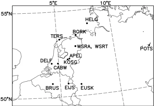
2.1 SD observations and their NWP model counterparts The SD observations used in this study are processed at the Technical University of Delft, the Netherlands. The observa-tions originate from 17 receiver staobserva-tions in the North-Western Europe over the time period 1–24 May 2003. Due to compu-tational limitations of the NWP model, a subset of 296 604 observations from 13 receiver stations, with a time interval of 10 min, is used. The receiver station locations are shown in Fig. 1.
The fundamental assumption behind the SD processing is that the fitting residuals of the geodetic network solution are indicative of the atmospheric asymmetry (de Haan et al., 2002). This assumption allows the usage of a two-step pro-cedure for processing. First, the symmetric component of SD is estimated as part of the network solution, using the least-squares fitting. Second, the fitting residuals are added on top of the symmetric component to obtain the final SD. Formally one can write
SD = mhZHD + mwZWD | {z }
Symmetric component
+δrs, (1)
where mhand mware the hydrostatic and wet mapping
func-tions, respectively, ZHD and ZWD are the zenith hydrostatic and wet delays, and δsr is the fitting residual, interpreted as the asymmetric component of SD, corresponding to the
satel-lite s and the receiver r. The processing applies the mapping functions proposed by Niell (1996).
The applied methodology for the processing has been criti-cised in geodetic literature. In particular, Elosegui and Davis (2004) showed by a simulation study, that the azimuthally asymmetric delay component cannot be completely retrieved from the fitting residuals of the network solution. Moreover, a gross measurement error in a single raw observation has a considerable impact on the other SD observations processed for the same receiver at the same time. This problem relates to general properties of any least squares fit, and it degrades the potential of the SD observations for any application, not only for NWP.
The model counterparts to the SD observations are pro-duced from the output of the High Resolution Limited Area Model (HIRLAM; Und´en et al., 2002). Three hour HIRLAM
forecasts are transformed from the model grid to the observa-tion space by applying the non-linear SD observaobserva-tion oper-ator (Eresmaa and J¨arvinen, 2006). The hydrostatic forecast model has been run with four different model resolutions. The initial state for the model integration is obtained by the three-dimensional variational data assimilation (3D-Var) sys-tem of HIRLAM (Gustafsson et al., 2001; Lindskog et al., 2001) separately for each model run. The SD observations have not been assimilated in the model. The first model run applies 40 model levels in vertical, horizontal grid spacing of 22 km and the operational analyses of the European Centre for Medium-range Weather Forecasts (ECMWF) as the lat-eral boundary condition. For the subsequent nested model runs, the grid spacing is halved in horizontal, and the lateral boundary conditions are retrieved from the NWP analyses obtained from the previous model run with a coarser grid. Consequently, the horizontal grid spacings in the nested runs are 11, 5.6 and 2.8 km, respectively.
Use of a non-hydrostatic NWP system, rather than the hy-drostatic HIRLAM system, would in theory be more justi-fied for horizontal grid spacings below 5 km (Niemel¨a and Fortelius, 2005). There is also a non-hydrostatic version of the HIRLAM model, but it is not applied here. This is moti-vated as follows: since the primary objective of running the model in a nested mode is to gain insight specifically into the role of the horizontal resolution in the SD modelling, the de-tails of the four model runs are kept as close as possible to each other. Different model dynamics and physical parame-terizations would be likely to confuse the interpretation of the results. Furthermore, since the area of interest is relatively flat and the studied period is not characterized by strong con-vective activity, the non-hydrostatic effects are believed to be weak. Role of the non-hydrostatic modelling is considered as a separate research issue, and it is not addressed in this study.
Fig. 1. The HIRLAMNWP model domain used in the run with grid spacing of 2.8 km. The GPS receiver station locations are marked with dots.
2.2 Determination of the asymmetric SD components Both the symmetric SD components and the fitting residuals are available in the present SD observation data set. There-fore, the asymmetric SD components would be readily avail-able for examination. In contrast, since the SD observation operator involves no least squares fitting, the NWP model counterpart data sets contain only the total SD values. For the sake of comparability, the asymmetric delay components from the observations and from the model counterparts are extracted in a similar manner using the following procedure. Note that the term “observable” is used here to refer to both the SD observations and the NWP model counterparts at the four horizontal grid resolutions.
1. The SD observables are classified in groups such that the observables at one receiver station at one time epoch constitute a group.
2. For each group, the SD observables are projected to zenith and averaged to yield a pseudo-ZTD, using a pre-determined mapping function.
3. The pseudo-ZTD is projected back to the actual satellite zenith angles to yield the symmetric component SDs of
each SD observable.
4. The asymmetric component SDais finally obtained by
subtracting SDsfrom SD.
Note that the resulting SDais not equal to δsr in (1), because
the determination of SDadoes not make use of separate
map-ping functions for hydrostatic and wet delay components.
Furthermore, a concept of asymmetricity rais introduced as
ra= |SDa|
SD (2)
associated to an SDa. ra is a measure of the azimuthally
asymmetric contribution to an SD observation or to a model counterpart.
Errors of the predetermined mapping function are recog-nized to contribute to the calculation of SDa even in a case
of a perfectly symmetric atmosphere. Specific attention is taken in order to find the mapping function that most accu-rately projects the SD observables to zenith (step 2) and back to the satellite zenith angle (step 3). Performances of hydro-static and wet mapping functions of Niell (1996) and Boehm et al. (2006) have been evaluated through histograms of SDa.
In principle, the better the mapping function, the narrower the histogram, and the closer is the mean SDa to zero. As
a result, the hydrostatic mapping function of Niell (1996) is selected for this study.
3 Asymmetricity in the SD observations
In this Section, a statistical approach is taken in order to fo-cus on the azimuthally asymmetric properties of the SD ob-servations. Mean value of asymmetricity raof the SD
obser-vations is 0.82 parts per thousand (ppt). Table 1 shows the numbers of the SD observations at different satellite zenith angle intervals, together with the percentages of those SD observations that exceed certain threshold values of raat
3146 R. Eresmaa et al.: Asymmetricity of ground-based GPS slant delay data
Table 1. Numbers of the SD observations (#SD) and percentages of
those observations that exceed the asymmetricity thresholds 0.5, 1, 2, and 3 parts per thousand (ppt) at different zenith angle intervals.
Interval #SD 0.5 ppt 1 ppt 2 ppt 3 ppt 0◦–5◦ 3566 64.2 36.3 8.10 1.37 5◦–15◦ 18365 62.3 33.2 6.98 1.24 15◦–25◦ 25901 59.0 29.3 5.15 0.76 25◦–35◦ 32047 56.9 26.4 3.92 0.46 35◦–45◦ 36842 56.0 25.5 3.64 0.44 45◦–55◦ 44382 57.2 26.5 3.93 0.57 55◦–65◦ 51088 59.0 29.1 5.47 0.97 65◦–75◦ 57822 64.4 36.4 8.74 1.77 75◦–80◦ 26591 71.2 46.2 15.4 3.91 0◦–80◦ 296604 60.5 31.3 6.47 1.21
the number of observations increases rather uniformly with increasing zenith angle. The first threshold, 0.5 ppt, is ex-ceeded by 60% of the observations, and nearly one third of the observations exceed the threshold of 1 ppt. About 1% of the observations exceed the threshold of 3 ppt. These per-centages depend on the satellite zenith angle interval. The observations at the largest zenith angles contain more asym-metricity than the other observations. From geometrical per-spective, this is not surprising, since those observations sense atmospheric regions farther away from the receiver station than the other SD observations.
Table 1 also indicates that the observations near zenith can be notably asymmetric. This is a rather surprising result, which could perhaps be explained as follows. The geodetic network solution is mostly contributed by the measurements from large zenith angles, because more satellites are visible there than near zenith. Consequently, the fitting residuals of the network solution appear to be large at small zenith angles. This phenomenon is solely due to the observing geometry and it has no relation to the atmospheric asymmetry.
The statistical behaviour of asymmetricity is studied also at separate GPS receiver stations. It is found that there are considerable differences between different receiver stations (not shown). The differences can be related to topographi-cal effects, such as land-sea distribution and orography, or to differences in the receiver station equipment, including re-ceiver and antenna types. Moreover, the effect of multipath propagation is highly dependent on the surroundings of the receiver. Unfortunately, the data set used in this study does not allow to draw any more specific conclusions on the re-ceiver station dependency.
Asymmetricity threshold of 3 ppt corresponds to an asym-metric delay component of about 7, 8 and 15 mm at the satel-lite zenith angles of 0◦, 30◦ and 60◦, respectively. The SD model counterpart error standard deviation is of nearly equal magnitude, but the SD observation error standard deviation is roughly 1.7 times larger (J¨arvinen et al., 2007). Thus, SD
0
10 20 30 40 50 60 70 80
ZENITH ANGLE [deg]
0.06
0.06
0.07
0.07
0.08
0.08
0.09
0.09
0.10
0.10
RATIO
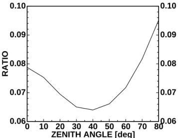
Fig. 2. Ratio of the standard deviations of the normalized
asymmet-ric and symmetasymmet-ric components of SD observations as a function of satellite zenith angle.
observation error standard deviation clearly exceeds the 3 ppt level of asymmetric delay component. Since the majority of the SD observations exhibits asymmetricity less than 3 ppt, the potential of the SD observations to NWP applications is somewhat doubtful. On the other hand, the representative-ness of the SD observations will increase through increasing NWP grid resolutions in the future. This is expected to de-crease the effective SD observation error from data assimi-lation point of view. Nevertheless, all efforts aiming at in-creasing the SD observation accuracy would be appreciated. These efforts might include advances, for instance, at the re-ceiver station equipment, increase in the accuracy of satellite orbit data, improvement in the treatment of the ionospheric refraction, or other breakthroughs in the SD processing pro-cedure.
Comparing the variabilities of the symmetric and asym-metric delay components provides another approach for as-sessing the asymmetric information content of the SD obser-vations. For this purpose, standard deviations of the sym-metric and asymsym-metric delay components are calculated at zenith angle intervals 0◦–5◦, 5◦–15◦, . . . , and 75◦–80◦. The delay components are normalized by the hydrostatic map-ping function of Niell (1996) prior to determination of the standard deviations. Figure 2 plots the ratio of the standard deviations of the asymmetric and symmetric delay compo-nents as a function of satellite zenith angle. The standard deviation of the asymmetric delay component appears to be between 6–10% of the standard deviation of the symmetric delay component. The shape of the curve, showing max-ima at both small and large zenith angles, is similar to the columns of Table 1. Overall, it is concluded that the variabil-ity of SD is mainly due to variabilvariabil-ity of the symmetric delay component.
0
2
4
6
8
10
ASYMMETRICITY [ppt]
10
10
10
10
10
FRACTION [%]
-3 -2 -1 0 1OBS
22km
11km
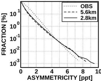
Fig. 3. Percentages of the SD observations and the model
counter-parts exceeding the given threshold of asymmetricity. Observations (dotted line) and model counterparts with a grid spacing of 22 km (dashed line) and 11 km (solid line).
4 Asymmetricity in the NWP model counterparts
In the previous section, the magnitude of the asymmetricity of the SD observations was studied in terms of percentages of observations exceeding certain threshold values. This Sec-tion provides a statistical comparison of the asymmetricity properties of the SD model counterparts with those of the SD observations. Comparison of single observations with their model counterparts will not be attempted yet. Motivation for this approach rises from properties of the analysis increments in data assimilation. The horizontal resolution of the analysis increments is governed by the so-called structure functions, which determine the spreading of information from observa-tions to the model grid, taking multivariate balances into ac-count (Berre, 2000). The structure functions are determined in a way, which leads to domination of synoptic scales in the analysis increments. The finer scale observational informa-tion is filtered out. The fine scale informainforma-tion in the analysis is provided solely by the background field and is generated by the forecast model through e.g. model physiography and land-sea distribution (Gustafsson et al., 2001).
The dotted line in Figs. 3 and 4 shows the percentages of the SD observations exceeding given thresholds. The statis-tics are calculated over all satellite zenith angles. Also the corresponding curves for the model counterparts with the four different horizontal grid resolutions are plotted. Fig-ure 3 shows the curves for the model run with 22 km (dashed line) and 11 km (solid line) grid spacings, and Fig. 4 shows the curves for 5.6 km (dashed line) and 2.8 km (solid line) grid spacings.
Among the large group of the most symmetric SD observa-tions, covering 99% of all cases, the observed asymmetricity
0
2
4
6
8
10
ASYMMETRICITY [ppt]
10
10
10
10
10
FRACTION [%]
-3 -2 -1 0 1OBS
5.6km
2.8km
Fig. 4. As Fig. 3, but for grid spacings of 5.6 km (dashed line) and
2.8 km (solid line).
is below 3 ppt. The model forecasts, especially those made with grid spacings 22 and 11 km (Fig. 3), fail to represent the asymmetricity to a similar extent in these cases and only reach 2 ppt. This could be explained by the SD observations containing a significant amount of non-meteorological mea-surement noise, resulting in too large asymmetricity in sym-metric atmospheric conditions. Another possible explanation is that the currently used NWP systems are unable to simu-late these small scale features. The fact, that an increase in the horizontal resolution results in closer agreement with the observations (Fig. 4), supports the latter interpretation. How-ever, without additional data it is not possible to exclude the former interpretation.
For asymmetricities above 3 ppt, the percentage curves of the model forecasts tend to approach the observation curve. At asymmetricity values higher than 5 ppt, the model coun-terparts with a 5.6 and 2.8 km grid spacing show even more asymmetricity than revealed by the observations. It is inter-preted that part of the asymmetric information is lost in the SD processing procedure in cases of extreme atmospheric asymmetricity. This interpretation is in line with the simu-lation study reported by Elosegui and Davis (2004), and it holds for 0.05% of the observations in the present data set.
Moreover, since the curves for the model counterparts with a 5.6 and 2.8 km grid spacing are very close to each other, it is concluded that the NWP grid with horizontal spacing of 5.6 km is likely to be dense enough in order to model the az-imuthal asymmetricity of the SD observations in the present data set with a reasonable accuracy. This means that data as-similation of the SD observations can be expected to be bene-ficial compared to data assimilation of the ZTD observations in NWP systems with horizontal grid spacing of around 5 km or less.
3148 R. Eresmaa et al.: Asymmetricity of ground-based GPS slant delay data
-0.01
0.00
0.01
ASYMMETRIC DELAY [m]
10
10
10
10
FREQUENCY
1 2 3 4OBS
22km
11km
-0.01
0.00
0.01
ASYMMETRIC DELAY [m]
10
10
10
10
FREQUENCY
1 2 3 4OBS
22km
11km
-0.04 -0.02 0.00 0.02 0.04
ASYMMETRIC DELAY [m]
10
10
10
10
FREQUENCY
1 2 3 4OBS
22km
11km
(a)
(b)
(c)
30
o50
70
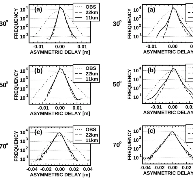
o oFig. 5. Frequency distributions of the asymmetric delay
compo-nents at zenith angle intervals 30◦±5◦(a), 50◦±5◦(b) and 70◦±5◦
(c). Observations (dotted line) and model counterparts with a grid
spacing of 22 km (dashed line) and 11 km (solid line).
Figures 5 and 6 show the frequency distributions of SDaat
three satellite zenith angle intervals. Figure 5 shows the dis-tributions of the SD observations (dotted line) and the model counterparts with a 22 km (dashed line) and 11 km (solid line) grid spacing, and Fig. 6 shows the distributions of the model counterparts with a 5.6 km (dashed line) and 2.8 km (solid line) grid spacing. At all zenith angle intervals, the distributions of the model counterparts are too narrow com-pared with the observed distributions. However, increasing the NWP model’s horizontal resolution generally increases the spread towards the observed distribution. At the zenith angle interval of 70◦±5◦, the distributions of the model coun-terparts at resolutions of 5.6 km and 2.8 km (panel (c) of Fig. 6) are very similar. On the other hand, the 2.8 km
reso--0.01
0.00
0.01
ASYMMETRIC DELAY [m]
10
10
10
10
FREQUENCY
1 2 3 4OBS
5.6km
2.8km
-0.01
0.00
0.01
ASYMMETRIC DELAY [m]
10
10
10
10
FREQUENCY
1 2 3 4OBS
5.6km
2.8km
-0.04 -0.02 0.00 0.02 0.04
ASYMMETRIC DELAY [m]
10
10
10
10
FREQUENCY
1 2 3 4OBS
5.6km
2.8km
(a)
(b)
(c)
30
o50
70
o oFig. 6. As Fig. 5, but for grid spacings of 5.6 km (dashed line) and
2.8 km (solid line).
lution provides clearly the best agreement with observations at the smaller zenith angles (panels (a) and (b) in Figs. 5 and 6). In conclusion, 5.6 km grid spacing appears to be suffi-cient for explicit modelling of the asymmetricities in the SD observations at the largest zenith angles, where the observed azimuthal asymmetricity is relatively large (see Table 1). De-creasing the grid spacing closer to 2.8 km is probably neces-sary in order to make the best use of the observations at zenith angles smaller than 65◦.
The frequency distributions of the model counterparts are generally not symmetric around zero. To be more specific, the distributions are skewed towards positive asymmetric de-lays at small zenith angles and towards negative asymmetric delays at large zenith angles. This behaviour can be seen also in frequency distributions corresponding to separate re-ceiver stations (not shown). Such a behaviour suggests that
the applied mapping function is inconsistent with the zenith angle dependency of the SD model counterparts. This is in line with the zenith angle dependent bias in the observation minus model background statistics reported earlier by Eres-maa and J¨arvinen (2006). This study applies no algorithm for bias correction. Note that it is impossible to say whether the observations or the model counterparts are more responsible for the bias. The symmetric distributions of SD observations in Figs. 5 and 6 most likely follow from the fact that the SD observation processing has made use of the same mapping function as the one applied in this study.
It is important to note that the asymmetric delay compo-nents of the model counterparts do not follow gaussian dis-tributions, while those of the SD observations do. It seems that the model counterparts contain too little asymmetricity in the relatively symmetric cases, but overestimate the asym-metricity in the cases of extreme asymasym-metricity. The reason for this behaviour is unknown at the moment.
5 Intercomparison in highly asymmetric cases
In this section, the comparison is extended to pairs of obser-vations and their model counterparts, focusing on cases of exceptionally high asymmetricity as revealed by either ob-servations or their model counterparts.
The asymmetricity rameasures the azimuthally
asymmet-ric contribution to an SD observation or to a model coun-terpart. Even though the high values of observed ra can be
attributed to atmospheric properties in the vicinity of the GPS receiver station, it is not obvious that all such cases are mete-orologically interesting. This is due to a number of uncertain-ties affecting the microwave propagation, signal reception and GPS data processing. In this Section, the NWP model forecasts are considered as reference atmospheres, which ei-ther do or do not support the interpretation of atmospheric properties as the source of high observed asymmetricity. 5.1 Support from the NWP model forecasts
In order to investigate whether the observed high asym-metricity values are signatures of atmospheric properties, the following procedure is applied:
1. The SD observations are ordered according to increas-ing ra. The observations exceeding the threshold ra
value of 3.12 ppt are considered highly asymmetric. The threshold is chosen such that the highly asymmetric ob-servations cover 1% of all SD obob-servations.
2. The model counterparts are ordered in a similar manner as the observations. The threshold value corresponding to 1% of the model counterparts varies between 2.19 and 2.65 ppt, depending on the horizontal grid spacing.
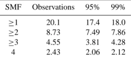
Table 2. Percentages, and their 95% and 99% confidence limits, of
highly asymmetric observations that are interpreted to indicate real atmospheric asymmetry at different numbers of supporting model forecasts (SMF). SMF Observations 95% 99% ≥1 20.1 17.4 18.0 ≥2 8.73 7.49 7.86 ≥3 4.55 3.81 4.28 4 2.43 2.06 2.12
3. The counterparts to the highly asymmetric observations, detected by the receiver station identification, observ-ing time and the Satellite Vehicle Number (SVN), are searched one by one from the group of highly asymmet-ric model counterparts. Time difference of up to three hours is allowed between the observation and the model background.
4. If there is a matching highly asymmetric model coun-terpart to the highly asymmetric observation, the NWP model is concluded to support the interpretation that this observation indicates a real atmospheric asymmetry. 5. The steps 2–4 are repeated four times corresponding to
the model counterpart data sets at four different NWP grid resolutions.
The interpretation of a highly asymmetric SD observation showing real atmospheric asymmetry is thus supported by up to four NWP model forecasts. The larger the number of supporting model forecasts (SMF) is, the more convincing is the interpretation. The second column of Table 2 shows the percentages of the SD observations receiving support of at least one, two, three or four SMF. A fraction of the highly asymmetric SD observations can be concluded to indicate a real atmospheric asymmetry. This result shows the balance between the noise influencing the SD processing and the me-teorological, azimuthally asymmetric, information contained in the SD observations.
5.2 Statistical significance of the support
It is obvious that the procedure described above would result in non-zero percentages in Table 2 even in a case of artificial SD observations being definitely independent of real atmo-spheric conditions. In other words, some unknown percent-age of the artificial observations would accidentally receive support from the NWP model forecasts and would further be concluded to show an asymmetric meteorological signal. Therefore, confidence limits to the percentages in Table 2 are estimated in the following way: A sample of one hundred sets of gaussian random numbers is constructed. Each set consists of 296 604 values being definitely not related to real
3150 R. Eresmaa et al.: Asymmetricity of ground-based GPS slant delay data atmosphere. Each individual random number in each set is
attached to one SD observation in the original data set; each random number is thus considered to represent asymmetric-ity of a single SD observation. The procedure applied above to the data set of observed asymmetricities is then applied one by one to each of the sets of random numbers. Repeat-ing the procedure over the sample of one hundred sets allows to assign the confidence limits. Note that the statistical pa-rameters of the random numbers are irrelevant for this study. The conclusions of the experiment will be sensitive only to the order at which the random numbers happen to occur.
The resulting 95% and 99% confidence limits are included in the third and fourth columns of Table 2 for each level of SMF. The percentage of highly asymmetric SD observations indicating real atmospheric asymmetry exceeds the 99% con-fidence limit at all SMF levels. The subsequent conclusion is that the SD observations contain a statistically significant asymmetric meteorological signal.
6 Conclusions
This article introduces and applies the concept of asym-metricity on the SD observations and their NWP model coun-terparts. Asymmetricity expresses the contribution of az-imuthal asymmetry to the total SD. On the basis of the results presented in the previous Sections, the following answers are provided to the questions listed in Sect. 1:
– How large is the contribution of the azimuthally
metric information to the SD observations? The asym-metric contribution, i.e. asymasym-metricity, is of the or-der of a few parts per thousand of the absolute delay value. In the extreme cases, mainly at satellite zenith angles larger than 65◦, the asymmetricity can exceed
the threshold of 5 ppt. It is exceptional that the asym-metric contribution is larger than the assumed standard deviation of the SD observation error.
– Is the azimuthal asymmetry in the SD observations
re-lated to real atmospheric asymmetry? As far as the NWP model represents the true atmosphere, it seems to be related. This conclusion holds for the cases of ex-treme asymmetricity and it is statistically significant at the confidence level of 99%.
– Are the currently operational NWP systems, with
hor-izontal grid spacings of around 10–20 km, able to rep-resent the scales appropriate for extraction of the asym-metric information? The HIRLAMNWP system is only partially able to represent the asymmetric properties of the SD observations. The closest agreement with the ob-servations is obtained at zenith angles larger than 65◦.
– Can the NWP model’s representation of the azimuthal
asymmetry be improved by increasing the horizontal
resolution? Yes, it can be improved. If the SD ob-servations at zenith angles larger than 65◦ are
consid-ered, the horizontal grid spacing of around 5 km seems to be dense enough in order to explicitly model the asymmetricity. However, modelling of the asymmetry at smaller zenith angles requires a denser grid.
This study makes use of a hydrostatic limited area NWP system, originally intended to provide synoptic scale guid-ance. It is possible that the conclusions would be some-what different if a finer scale non-hydrostatic NWP system was used. Moreover, the results are expected to depend also on the horizontal resolution of the observing systems assim-ilated in the model.
The currently operational limited area NWP systems are already close to the highest horizontal resolution used in this study. Therefore, the NWP data assimilation is expected to be able to make use of the whole information content of the SD observations in near future. At the moment, the most obvious obstacle for SD data assimilation is the lack of data processing in near real time.
Acknowledgements. The funding from the EU FP5 project
“Targeting Optimal Use of GPS Humidity Measurements in Me-teorology” (TOUGH) in 2003–2006 and from the TEKES project “Geophysically Assisted Satellite Positioning” in 2004–2006 is thankfully acknowledged. TOUGH is a shared-cost project (contract EVG1-CT-2002-00080) co-funded by the Research DG of the European Commission within the RTD activities of the Environment and Sustainable Development sub-programme (5th Framework Programme). TEKES is the Finnish Funding Agency for Technology and Innovation. The authors are grateful for Hans van der Marel (Technical University of Delft, the Netherlands) for providing the SD observations.
Edited by: K. Hamilton
References
Berre, L.: Estimation of synoptic and mesoscale forecast error co-variances in a limited area model, Mon. Wea. Rev., 128, 644– 667, 2000.
Bevis, M., Businger, S., Herring, T., Rocken, C., Anthes, R., and Ware, R.: GPS meteorology: Remote sensing of atmospheric water vapor using the Global Positioning System, J. Geophys. Res., 97, 15 787–15 801, 1992.
Boehm, J., Niell, A., Tregoning, P., and Schuh, H.: Global Mapping Function (GMF): A new empirical mapping function based on numerical weather model data, Geophys. Res. Lett., 33, L07304, doi:10.1029/2005GL025546, 2006.
Bouttier, F.: The AROME mesoscale project, in: Proceedings of a seminar on Recent developments in data assimilation for at-mosphere and ocean, 8–12 September 2003, European Centre for Medium-Range Weather Forecasts, Shinfield Park, Reading, Berkshire, England, pp. 433–448, 2004.
de Haan, S., van der Marel, H., and Barlag, S.: Comparison of GPS slant delay measurements to a numerical model: case study of a cold front passage, Phys. Chem. Earth, 27, 317–322, 2002.
De Pondeca, M. and Zou, X.: A case study of the variational assim-ilation of GPS zenith delay observations into a mesoscale model, J. Appl. Meteorol., 40, 1559–1576, 2001.
Elgered, G., Plag, H.-P., van der Marel, H., Barlag, S., and Nash, J., eds.: COST Action 716: Exploitation of ground-based GPS for operational numerical weather prediction and climate appli-cations, Final report, Rep. EUR 21639, European Union, 234 pp., 2005.
Elosegui, P. and Davis, J.: Accuracy assessment of GPS slant-path determinations, in: Proc. International Workshop on GPS mete-orology, Tsukuba, Japan, 14–17 Jan 2003, edited by: Iwabuchi, T. and Shoji, Y., 1-35-1–1-35-6, 2004.
Eresmaa, R. and J¨arvinen, H.: An observation operator for ground-based GPS slant delays, Tellus, 58A, 131–140, 2006.
Gustafsson, N., Berre, L., H¨ornquist, S., Huang, X.-Y., Lindskog, M., Navascu´es, B., Mogensen, K. S., and Thorsteinsson, S.: Three-dimensional variational data assimilation for a limited area model. Part I: General formulation and the background error con-straint, Tellus, 53A, 425–446, 2001.
Ha, S.-Y., Kuo, Y.-H., Guo, Y.-R., and Lim, G.-H.: Variational as-similation of slant path wet delay measurements from a hypothet-ical ground-based GPS network. Part I: Comparison with pre-cipitable water assimilation, Mon. Wea. Rev., 131, 2635–2655, 2003.
Hollingsworth, A., Viterbo, P., and Simmons, A. J.: The relevance of numerical weather prediction for forecasting natural hazards and for monitoring the global environment, Tech. Memo. 361, ECMWF, European Centre for Medium-Range Weather Fore-casts, Shinfield Park, Reading, Berkshire, England, 29 pp., 2002. J¨arvinen, H., Eresmaa, R., Vedel, H., Salonen, K., Niemel¨a, S., and de Vries, J.: A variational data assimilation system for ground-based GPS slant delays, Q. J. Roy. Meteor. Soc., in press, 2007.
Lindskog, M., Gustafsson, N., Navascu´es, B., Mogensen, K. S., Huang, X.-Y., Yang, X., Andræ, U., Berre, L., Thorsteinsson, S., and Rantakokko, J.: Three-dimensional variational data assimi-lation for a limited area model. Part II: Observation handling and assimilation experiments, Tellus, 53A, 447–468, 2001.
Liu, H. and Xue, M.: Retrieval of moisture from slant-path water vapor observations of a hypothetical GPS network using a three-dimensional variational scheme with anisotropic background er-ror, Mon. Wea. Rev., 134, 933–949, 2006.
MacDonald, A. E., Xie, Y., and Ware, R. H.: Diagnosis of three-dimensional water vapor using a GPS network, Mon. Wea. Rev., 130, 386–397, 2002.
Niell, A.: Global mapping functions for the atmosphere delay at radio wavelengths, J. Geophys. Res., 101, 3227–3246, 1996. Niemel¨a, S. and Fortelius, C.: Applicability of large scale
con-vection and condensation parameterization to meso-γ -scale HIRLAM: A case study of a convective event, Mon. Wea. Rev., 133, 2422–2435, 2005.
Und´en, P., Rontu, L., J¨arvinen, H., Lynch, P., Calvo, J., Cats, G., Cuxart, J., Eerola, K., Fortelius, C., Garcia-Moya, J. A., Jones, C., Lenderlink, G., McDonald, A., McGrath, R., Navascu´es, B., Woetman Nielsen, N., Ødegaard, V., Rodriguez, E., Rum-mukainen, M., R˜o˜om, R., Sattler, K., Hansen Sass, B., Savij¨arvi, H., Wichers Schreur, B., Sigg, R., The, H., and Tijm, A.: HIRLAM-5 Scientific Documentation, Hirlam-5 Project, avail-able from Hirlam-5 Project, c/o Per Und´en, SMHI, S-60176, Norrk¨oping, Sweden. 144 pp., 2002.
Vedel, H. and Huang, X.-Y.: Impact of Ground Based GPS Data on Numerical Weather Prediction, J. Meteor. Soc. Japan, 82, 459– 472, 2004.