HAL Id: halshs-00564688
https://halshs.archives-ouvertes.fr/halshs-00564688
Preprint submitted on 9 Feb 2011HAL is a multi-disciplinary open access
archive for the deposit and dissemination of sci-entific research documents, whether they are pub-lished or not. The documents may come from teaching and research institutions in France or abroad, or from public or private research centers.
L’archive ouverte pluridisciplinaire HAL, est destinée au dépôt et à la diffusion de documents scientifiques de niveau recherche, publiés ou non, émanant des établissements d’enseignement et de recherche français ou étrangers, des laboratoires publics ou privés.
Emission: Reduced vs. Structural form and the role of
international trade
Jie He
To cite this version:
Jie He. Economic Determinants for China’s Industrial SO2 Emission: Reduced vs. Structural form and the role of international trade. 2011. �halshs-00564688�
Document de travail de la série Etudes et Documents
Ec 2005.05
ECONOMIC DETERMINANTS FOR CHINA’S INDUSTRIAL SO2EMISSION:
REDUCED VS.STRUCTURAL FORM AND THE ROLE OF INTERNATIONAL TRADE
Jie HE
CERDI
University of Auvergne 65, Boulevard François Mitterrand
63000 Clermont-Ferrand France Tel : +33-4-7317-7501 Fax : +33-4-7317-7428 Email : Jie.HE@u-clermont1.fr February 2005 36 p.
Abstract
In this paper, basing on panel data on Chinese provincial level from 1991-2000, we test, firstly, the existence of EKC for industrial SO2 emission density. Following, we decompose the economical
determinants of this SO2 emission density into: income effect (GDPPC), scale effect (Industrial GDP per
km2) and composition effect (industrial capitalistic ratio). And in the third step, we study the direct and indirect role of international trade intensity ((X+M)/GDP). Instead of a supposed EKC, we find ever-increasing trend in industrial SO2 emission density with respect to income growth for most Chinese
provinces when the three largest cities (Beijing, Tianjin and Shanghai) directly under central government are taken off from our database. Following, confirming Grossman (1995), we succeed in decomposing industrial SO2 emission density into its three famous economic “effects”. However, different from our
expectation, the composition effect, measured by industrial capitalistic ratio K/L in this paper, instead of being a pollution-increasing role as generally accepted idea, turns out to lead industrial SO2 density to
reduce as a technology-reinforcing factor. For the role of trade, besides the positive direct impact on industrial SO2 density, we find equally some “pollution haven” evidences. In addition, our results show
for most provinces, their comparative advantage stays still in labour-intensive sectors, increase in the capitalistic ratio is proven to be environment-friendly through its technological “pollution-abatement” effect until this ratio reach the level of 83333 yuan/person, which can be considered as the threshold to distinguish capital-intensive sector. Due to these different aspect’s effects, corresponding to the conclusion of ACT (1998, 2001), the total effect of trade on industrial SO2 pollution does not turn out to
be an important factor for industrial SO2 emission density. Including all these co-related economic
determinants into a more general graphical analysis, we find that, for most provinces whose actual income and capitalistic ratio stay still at moderate level, further income growth and capital accumulation are generally environment-friendly factor in openness process. However, the further enlargement of openness degree will result in environment deterioration for the provinces that have relatively low income and too low or too high capitalistic ratio. The necessary policy to reduce this possible deterioration is to adopt besides the open policy, the complementary policies aiming at reinforcing public consciences on environment quality (through income effect) and encouraging R&D activities to increase technological efficiency in pollution abatement.
Key Words: China, EKC, international trade, industrial SO2 emission, decomposition, “pollution haven”
1. Introduction
China, one of the countries with highest growth rate, risks equally to be nominated as one of the most polluted countries in the world. With the increasing importance attached to environment in development process and the common understanding achieved on the definition of sustainable development, how to realize economy growth without arousing environment deterioration and future potential growth capacity lose becomes an important topic for Chinese economy studies.
According to Selden and Song (1995) and Lopez (1994), given accelerating increase in marginal “disutility” caused by pollution with income level and the ever-strengthening “substitutability” between clean and dirty production technologies, the disutility from environmental deterioration will finally become enough serious to make cleaner production technologies necessary measure for utility maximization objective. Therefore theoretically, the appearance of the dichotomy between economy growth and environment degradation described in EKC hypothesis can be automatically realized when income attains certain critical threshold.
Although over twenty empirical analyses on cross-section data showed evidence for this dichotomy between economy growth and environmental deterioration during growth process. This ex-post relationship between economy growth and environment for certain countries and certain periods found in reduced form cannot offer us more information about how to improve environment without sacrificing economy growth. Furthermore, from a strict econometrically point of view, the environment-growth relation found in the reduced form is probably spurious, since the two variables follow obviously some opposite trends during the time. In addition, the disagreement between these studies on the actual form of EKC also brings difficulties in extrapolating the static EKC found by cross-country experiences into a dynamic projection for the relation between environment and economy growth for a single country, especially a developing countries like China, who appears relatively less frequently in these studies. Even if the extrapolation were possible, the income level corresponding to the turning points of these cross-country EKC (5000-8000 USD, Dasgupta et al, 2002, 1990 price) are generally too high with respect to China’s current income level (4534 yuan, 947.78 USD equivalent in year 2000 ).i Whether deterioration in environment in China is an unavoidable price for economical growth? Whether such a high income
Common (2000) said, the global EKC is, at least for the case of SO2 emission, a “misspecification”, each
country in fact, has its own special trajectory formed in her special historical, geographical, political and economical conditions?
Instead of staying at the reduced form of EKC, economists also try to search more direct links between economic activities and pollution. Grossman (1995) regarded pollution as a by-product of production activities and can be calculated by multiplying the output of each sector with its pollution intensity and then sum them up. According to him, the economic determinants for pollution emission can be classified into three effects. The scale effect, supposing the emission rate unchanged, larger is the production scale of one economy, more pollution she emits to environment. The composition effect, given emission intensity and industrial scale stay unchanged, more industrial composition deviates to pollution-intensive sectors, more pollution will be emitted. And finally the income effect (or technique effect), which suppose an increase in income will reinforce on one hand, public demand for better environment, and on the other hand, permits improvements in pro-environment research and development activities, given industrial scale and composition of this economy unchanged, income increase will reduce pollution. This decomposition in fact shows a dynamic version to explain the formation of EKC during one country’s economic growth process. When the positive link between industrial scale and pollution is cancelled off by the pollution reduction effect from income increase and industrial composition transformation, the famous dichotomy between environment and economy will appear. As concluded in Panayotou (1998): “the apparition of one EKC results from a J-curve relationship between pollution abatement expenditure and income level masked by scale and composition effect”.
However, the pessimists pointed out that the EKC found by cross-section data are possibly showing only a static “pollution haven” effect caused by trade liberalization, the latter works as a canal for developed countries to discharge their environmental burdens to developing ones. If this is true, from a global point of view, environment pollution has not reduced in volume but only transfer from rich countries to poor ones. However, last ten years’ empirical studies have not achieved agreement on this issue. On one hand, many empirical analyses did not find evidences to support this predicted negative relationship between openness and environmental quality, like Tobey (ACT, 1990), Grossman and Krueger (1991), Agras and Chapman (1999) and Antweiler, Copeland and Taylor (2001). Their results
pass on the information that, whatever is its implication in pollution, “the trade’s impact --whether positive of negative-- will be small”. On the other hand, there also exist the studies supporting the hypothesis of “pollution haven”. Hettige et al (1992) found that, the reduction in industrial toxicity intensity in sense of total GDP in developed countries was not realized by an absolute reduction in toxicity intensity with economic growth, but by the displacement of their pollutant industries to the low income countries, since the industrial toxicity intensity per unit of industrial output in these developed countries has not declined with their total volume reduce during the time. Rick (1996) proved that the chemical toxicity intensity is higher in the countries applying “outward-orientation” trade strategies than those following “inward-orientation” trade strategies. By studying in detail on the actual product movements between countries, Suri and Chapman (1998) also concluded the apparition of an EKC between countries of different income levels is due to the fact that the industrialized countries satisfy their consumption demand for the energy-intensive products by importing them from industrializing countries instead of producing themselves.
The incoherence between these empirical results reflects the potential complexity in the environment/openness nexus. Besides the differences in the strictness of environmental regulations, there are also other aspects through which international trade can influence pollution, such as the differences in economical, natural endowment and institutional characteristics between countries. There should not exist a general version for the environment/openness relationship that can be applied easily to different economies.
Comparing to developed countries, China is, at the same time, rich in labor forces endowment and relatively poor. The reasoning of Copeland and Taylor (1997) shows that, on one hand, China’s natural comparative advantages should lead her to participate in international division system by specializing in labor-intensive sectors which is supposed to be less pollution-intensive; on the other hand, “pollution haven” hypothesis expects China’s relatively relaxing environmental regulations due to her low income also endows her with some comparative advantages in pollution-intensive sectors. The total effect of trade on environment should depends on the forces contrast between the “pollution haven” effect, which attracts polluting sectors, and the composition effect, which favors the growth of less polluting
In this paper, after a quick description on Chinese current economical and environmental situation and data discussion, we will firstly test the existence of a reduced-form EKC for industrial SO2 emission
density by using the panel data on Chinese provincial level from 1991 to 2000. For a better understanding of the structural determinants of Chinese environmental quality, following, we decompose the three determinants defined by Grossman (1995) for industrial SO2 emission. Following, to analyze the direct
and indirect role of international trade in emission determination, we include into our estimation model the trade intensity (defined as the ratio of international trade to GDP of the same period) individually and interactively with the other structural determinants. Finally, we conclude.
2. An introduction on the actual Chinese economical and environmental situation
(1) China’s economic situation during her economy reform
During the 1990s, China experienced an obvious tendency of economy growth. According to China’s official statistical data, the real average growth rate of GDP was 8.7% during 1990-2000. The per capita GDP almost tripled in the last decade, from 1634 Yuan of year 1990 to 4534 Yuan of year 2000. However, in term of the absolute level of income per capita, China is still a low-income country with a per capita GDP of 947.78 USD (2000 price) in the year 2000 according to the official exchange rate.
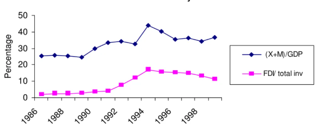
Like most of the East Asian industrializing countries, China’s economy growth showed a remarkable increase in industrial activity ratio to the whole economy during the last two decades, from 37% of year 1990 to 52% of year 1999 (China’s Statistics Yearbook, 2001). The openness policy since 1978 has induced a rapid integration of Chinese economy into the world market, which is not only presented by the increase in the ratio of international trade to GDP, but also by huge inflows of foreign direct investments. Figure 1 shows the common up-growing tendency in trade intensity (defined as the sum of export and import over total GDP) and FDI intensity (defined as the ratio of FDI in China over total fixed investment). These two ratios experienced firstly a rapid increase in the first half of 1990s, and then stayed relatively steady at this high level in the second half.
(Insert Figure 1 about here)
(2) China’s environmental situation during her economy reform period
Besides a remarkable progress in economy growth process, we noticed at the same time, serious environmental pollution problems in China. The SO2concentration indices in the large Chinese cities are
very high, even according to the standards for developing countries. For many large Chinese cities, their SO2 concentration level during 1996-1997 is at least twice higher than the standard of World Health
Organization (WHO) for developing countries. In Guiyang, the index of concentration of SO2 is even 7
times higher than the standard (China’s Environmental Statistics, 1998).
Although the situation of SO2 concentration in urban regions is serious, fortunately, we observed
during the same period amelioration tendency in industrial SO2 emission intensity. Showed in Figure 2,
since 1990, the increasing tendency of industrial SO2 emission ran slowlier than that of industrial output,
which in fact indicates an actual decreasing tendency in industrial SO2 emission intensity.
(Insert Figure 2 about here)
(3) The great disparity in economic growth and environmental situation between provinces
Due to the tradition to give local government relatively more autonomy in economic policy decision and the great differences in geographical, political and historical characters between provinces, the inter-province disparity is a remarkable character for Chinese regional economy. In figure 3, we enumerate the income level, trade intensity and industrialization degree in year 1998 for seven chosen representative provinces.ii Obviously, the differences are striking, especially for the income level and integration degree. In figure 4, similar to their economic characters, the annual industrial SO2 emission
situation in the seven chosen provinces is also very different, so are their variation tendency during year 1992 to 1998.
(Insert Figure 3 and 4 about here)
3. Environmental indicator
We choose industrial SO2 emission as environmental indicator studied in this paper. This choice is
based on two considerations. Firstly, since most of the previous empirical EKC studies discussed the SO2
pollution case in their works, by concentrating on SO2 pollution, we can get more reference for our
results. Secondly, SO2 emission is the most important air pollution problem in China. Moreover,
industrial SO2 emission is responsible for 70% of the total SO2 emission in China (World Bank, 1998).
By concentrating on industrial SO2 emission, weshould be able to get better understanding on China’s air
However, instead of using the emission per capita as dependant variable as many paper discussing the similar topic, in this paper, we decided to calculate the emission density for each province by dividing the annual emission with the surface of the corresponding province. Doing so, without losing the principal characteristic of total industrial SO2 emission for each province as the geographical area of each
province is constant during years, we have an environment indicator similar to pollution concentration index. In addition, comparison between the environment indicator of emission per capita and emission per km2 in equation shows the difference resides on the fact that the population density information is in fact missed in the emission per capita indicator. Since the same quantity of emission can cause more health problem if the population are more condensed in a smaller surface. We will have more interest to choose emission per km2 as environmental indicator from the point of view of the impacts of pollution on economy’s capacity of sustainable development, such as health impact of pollution that can cause the reduction in labor’s productivity. Furthermore, this calculation will also permit us to avoid the disturbances in our estimation coming from the huge geographical dimension difference between provinces. density Population Population Emission Area Population Population Emission Area Emission= × = × (1)
Table 1sum up the statistics for all the data used in this article. (Insert Table 1 about here)
4. The existence of EKC —“reduced form” analysis
To estimate firstly the existence of an “inverted U” relationship between industrial SO2 emission
density and income per capita, we employ a simple reduced form to connect industrial SO2 emission
density (SO2it) directly to GDP per capita (GDPPCit) as equation (2).
it 3 2 it 2 it 1 i it 2 X GDPPC (GDPPC ) t SO = +
α
+α
+α
+ε
(2)The index i and t represent respectively province and year. Given great inter-provincial differences in economic and environmental situation, we use Xi to capture the immeasurable and unchanged specific
effect for province i. At the same time, to capture the possible time tendency in emission, we add also in our estimation t, a time trend variable.
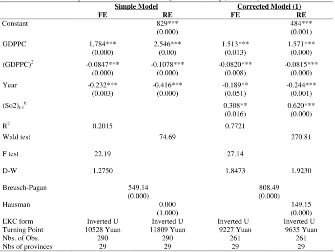
Table 2 presents the main results for EKC estimation. The Simple Model columns record the estimations based directly on Eq(1) and the Corrected Model columns include the results after correcting the first order serial-correlation problems within each group by including the instrumented lagged dependant variable SO2it-1 on the right hand of the regression function.
iii
Basing on this reduced form, we do find a significant inverted U form relationship between emission and GDPPC with the turning point close to 10000 CNY (about 2090 USD).iv However, the relatively low R2 value shows only the income level has in fact weak explication power for industrial SO2 pollution.
(Insert Table 2 about here) (Insert Figure 5 about here)
The figure 5 shows graphically the found Environment Kuznets Curve based on the result in Table 2.v Given that we accept these Environmental Kuznets Curves, what are the actual positions of the 29 provinces on this inverted U form curve? In Table 3, we show income level in year 2000 for each province and their geographical area. Interestingly, except the three municipalities directly under central government as Shanghai, Beijing and Tianjin, the income level of the other 26 provinces is still below the threshold of 10000 CNY. At the same time, the geographical areas of the three municipalities are also the smallest among 29 provinces (and cities). Therefore, their SO2 density will be naturally higher than that
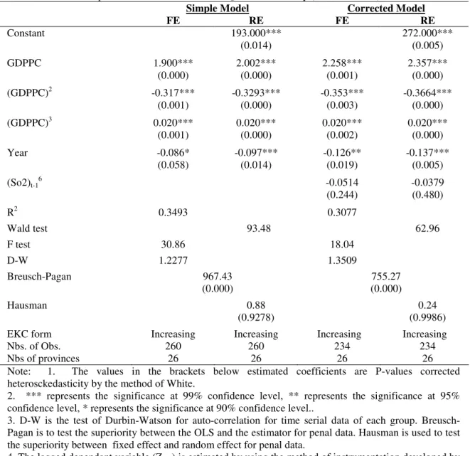
of the other provinces due to their higher concentration of economic activities, a general characteristic for urban economy. Correspondingly, in Figure 5, most observations are actually concentrated in the increasing part of the curve and the points corresponding to the decreasing part of EKC is only the several ones belonging to the largest municipalities whose income level is higher than that corresponding to the turning point. Whether the found inverted U curves are in fact formed by the overwhelmingly increasing part of the 26 provinces whose industrialization process is on progress and the distorted “pulled-down” part beyond the income level of 9000-10000 Yuan by the outlier observations of the three special municipalities whose economy structure is beginning to deviate to services and high-tech sectors? To test this possibility, we re-estimate the EKC hypothesis in the sub-sample of 26 provinces. The results are presented in Table 4.vi
Interestingly, after reducing the database to only 26 provinces, the previous inverted U curve for industrial pollution density with respect to income disappears. The right panel of Figure 6 plots separately the industrial SO2 density of the three municipalities to their respective income level. Only Shanghai and
Beijing have clear decreasing tendency in their industrial SO2 emission density, even the 10 observations
of Tianjin still keep an increasing trend for SO2 density with income growth. Whether we can conclude
that the increasing tendency in the 26 provinces and Tianjin is in fact due to their income level are still below the critical threshold level of 10000 Yuan, and further income increase in these provinces will finally help to realize the dichotomy between economy growth and environment deterioration as that happened in the two most rich Chinese municipalities? Or the inverted U curve found in Table 2 is only an increasing curve for Chinese provinces distorted and pulled down by the “large city effect”? To answer these questions, we go further to employ a structural model and look into the other economic determinants of industrial SO2 density besides per capita GDP.
(Insert Table 4 about here) (Insert Figure 6 about here)
5. The economic determinants of industrial SO2 emission density — a structural model and the
decomposition step
(1) Relationship between industrial SO2 emission intensity and income
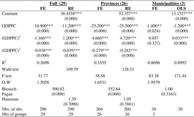
Since income growth can reinforce both demand and supply capability of an economy for better environment, Selden and Song (1994) and Panayotou (1998) have directly considered per capita GDP as an indicator for abatement activities. In this section, we also look into the direct relationship between income and SO2 intensity (measured by SO2 divided industrial GDP). The estimation results are in Table
5. Corresponding to the last step, our estimation also consists of three parts, the results based on full sample, on 26-province restricted sample and on 3-municipality sample. Figure 7 gives the graphical demonstration of the estimated relationship. Different from the case of SO2 density, in all the three
samples we find the common decreasing tendency in industrial SO2 intensity with respect to income
growth. This finding reminds us the quite similar results of Hettige et al (2000, p460) and confirms that of Selden and Song (1995) and Panayotou (1998). It does reflect the significant technological progress tendency in cleaning production in Chinese industrial sector.
(Insert Table 5 about here)
(Insert Figure 7 about here) (2) Grossman decomposition
If we agree that emission is a by-product of production, according to Grossman (1995), the density of industrial SO2 emission can be decomposed into the following three determinants.
)
Y
SO
Y
Y
(
area
Y
area
SO
i i 2 i i 2=
∑
×
(3)The index i=1, …, n signifies different industrial sectors. Y presents industrial GDP and area means geographical area. The first term (Y/area) reflects industrial activity density, signifying scale effect in Grossman’s definition. A higher industrial activity density normally means higher pollution density if SO2 emission intensity keeps constant. (Yi/Y), the proportion of product of sector i in total industrial
product reflects the composition effect in Grossman (1995). Intuitively, the industry composition with higher proportion of pollution industry has a higher pollution density if the other determinants keep unchanged. Finally, (SO2i/Yi) means pollution intensity of sector i. If industrial scale and composition
hold constant, higher pollution intensity leads to more pollution. This determinant is also called by Grossman as income effect, since he supposes income growth can lead pollution intensity to decrease, which is already confirmed by our previous results. Therefore, we can re-write the equation (3) as following by replacing the intensity term by GDPPC.
( )
e
GDPPC
Y
Y
area
Y
area
SO
i i i 2=
∑
×
×
(4)ei is a sector specific factor for SO2 intensity, we use it to capture the specific emission characters
in different sector since GDPPC can only reflect the general correlation of income level with the average industrial SO2 intensity of total economy and ignore the possible sectoral specific character in emission
intensity. From equation (4) we see that GDPPC is only one of the determinants for SO2 emission density
besides the scale effect (Y/area) and composition effect
∑
×
i
i i
/
Y
e
)
Y
(
. The divergent tendency betweenindustrial SO2 emission density and per capita income (or more directly, industrial SO2 emission
structural determinants in industrial SO2 emission density besides GDPPC. Followed, we use the
estimation function (5) to see the possible contribution of these two economic determinants.
it i it it it it 2 GDPPC Scale (K /L) X t SO =β +γ +θ +φ +ρ +ε (5) Besides GDPPC measuring the income effect, provincial total industrial GDP over the surface of the same province is used to measure the scale effect (Scaleit). We expect a positive coefficient for it. To
avoid data constraints in constructing a detailed composition effect indicator due to insufficient information in the sector specific factor ei, we use total industrial capitalistic ratio (K/L) to describe
industrial composition for each province by simply supposing a sector more capital-intensive to be generally more pollution-intensive. The same hypothesis can be found in Copeland and Taylor (1994, 1997) and ACT (2001). Therefore, for this variable, a positive efficient is expected. To include the provincial specific effect, we employ penal data estimator for this equation. Considering the possible non-linear relationship between industrial SO2 emission density with these determinants, we include the
higher order polynomial terms when necessary.
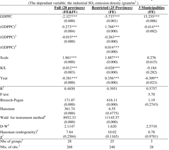
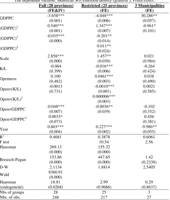
The estimation results are in Table 6. Similarly, the estimations are done in three samples: full (28 provinces & cities, we drop Hainan province due to lack of investment indices for this province), 25 provinces and 3 municipalities. Clearly, included the other two variables, the model’s explication power is improved (from 0.20 to 0.39). Moreover, since Wang and Wheeler (1996), World Bank (2000) indicated that “China’s levy system has been working much better than that has been supposed” due to her great flexibility and her active complaining citizens, we wonder whether this effective levy system (official or non-official) will in turn result in some feedback effect in re-orientation of the new production capacity investment and then in industrial composition formation given some sectors are more pollutant than the others. To test the potential simultaneity or endogeneity in composition and scale effect with respect to the industrial emission density, we use the lagged composition effect (K/L)it-1 and lagged scale
effect (Scale)it-1 as instruments for current (K/L)itand (Scale)it in each of the result reported in Table 6.
The Hausman test (1978) is used to compare the efficiency of the instrumental method with that of the estimations without instruments. Confirming to the opinion about the high efficiency of Chinese emission levy system, the χ2 value of Hausman (1978) test proves the endogeneity of the scale and composition effect in the full 28 provinces and especially in the 25 provinces sample.
(Inserted table 6 about here)
Further comparison in the three columns in Table 6 shows, interestingly, the estimation results of the full and 25-province restricted samples tell very different stories than that from 3 cities. Though for the 3 cities, the relationship between emission density and income level keeps the same inverted U form with the downward turning points at the income level of 18424 yuan. The results for the full sample shows that income growth seems to lead SO2 emission density to decrease by reducing SO2 emission
intensity. While for the 25-province sample, the relationship between income effect and SO2 emission
density for 25-province sample is in fact a U-formed curve, with the upwards turning point at about the GDPPC of 7600 yuan, which is generally beyond the income of most of the 25 provinces in the sample. Therefore, we can still suppose the income effect as a monotonous reduction factor for industrial SO2
emission density for these 25 provinces.
Concerning the two new explication factors for SO2 emission density, their significant coefficients
for the full and 25-province samples and not for the 3 municipalities shows the potential difference in the determination mechanism of industrial SO2 emission density between the 25 provinces and the 3 cities.
Given a generally negative relationship between income growth and industrial SO2 intensity, the
significance of the scale and composition effect in the results of the 25 provinces show the determination forces of industrial SO2 emission in these provinces come principally from production activity. While for
the 3 cities, the only significance found for income effect shows that industrial pollution in these cities is actually related to people’s consumption demand going up with income growth rather than their production activities.
Another finding need to indicate is that, in all of the three estimation results, contrary to the generally accepted idea that higher capitalistic ratio means more serious pollution performance, our results show the increase in industrial capitalistic ratio leads to, significantly, a decrease in industrial SO2
pollution. We will come back with more detail to this point in the following section.
6. The role of international trade in determination of industrial SO2 emission density
ACT (2001) succeeded in merging the role of openness into the decomposition model similar to Grossman (1995). Following their reasoning, we assume that international trade can exert influence on
low income with respect to her rich trade-partners will make her attractive for investment in pollution-intensive production, and on the other hand, the traditional comparative advantage hypothesis that assumes China’s richer endowment in labor forces also leads her to specialize in labor-intensive sectors, which are generally regarded as less pollution-intensive. Therefore, the total effect of trade on environment of one province depends on the force contrast between her industrial composition characters and her income level.
Following the empirical idea of ACT (1998, 2000) and basing on the decomposition in the last section, we look further into the trade impacts on in industrial pollution in Chinese provinces in this section. To capture the impacts of trade on industrial SO2 emission density, we will firstly introduce
simply the trade intensity variable (openit), measured by the ratio of sum of export and import over total
GDP of each province.vii In turn, for a better understanding on the indirect effects of trade that depend on the provinces’ income level and industrial composition characters, we further add into our estimation function the interaction terms between the openness and the two effects, (open×(K/L)) and (open×GDPPC). “Pollution haven” hypothesis supposes with the same openness degree, lower is the income level for a country, she has more pollution problem, so a negative coefficient for (open×GDPPC) term confirms this hypothesis. The traditional comparative advantage theories shows a country endows more labor will have less pollution problem under trade liberalization since their comparative advantage is in the labor-intensive sectors which are generally considered to be less pollution-intensive. Therefore for the multiple terms between trade and industrial capitalistic ratio, a positive coefficient means confirmation to the traditional international trade hypothesis.
The results are shown in Table 7. Coherent to the results found in decomposition step, the coefficients of income effect keep the same significance and the expected signs in all the three samples. The scale effect, similar to last decomposition step, shows its positive and significant coefficient only in full and 25-province restricted samples. Come to the composition effect, we only find its determination role in 25-province sample with a significantly negative coefficient, which is, once more, contrary to the general accepted expectation of a positive relationship. For the full and 3-municipality sample, the role of the capitalistic ratio turns out to be non-concludable due to their unsatisfactory P values.
Come to the role of trade, we find the direct effect of international trade is significantly positive in the full and 25-province restricted sample. This indicates increase in openness degree can directly bring more pollution. Similar to ACT (1998, 2001), for full and 25-province restricted samples, the inclusion of the multiple terms of trade with income and composition effects can not improve the efficiency of estimation until the quadratic terms (open×GDPPC2
for full sample estimation and open×(K/L)2
for the 25-province restricted sample estimation) are included. While for the 3-municipalitiy sample, the inclusion of trade terms and the multiple terms of openness degree fails once more to improve the explication power of the estimation The only determination role residing in income level reveals for once more the consumption-determination mechanism for industrial SO2 emission in the three largest cities.
Though there exist small differences in the estimation results of the trade terms between full and 25-province restricted samples, the coefficients of the multiple terms of trade with income and composition effect between full and 25-province restricted samples show good coherence. The negative coefficients before the open×GDPPC terms confirm “pollution haven” hypothesis. However, this decreasing tendency in pollution with income increase seems not to be monotonous, since in full sample, once income level goes beyond 7273 yuan/person, further income growth leads pollution to retake the increasing tendency. This in fact corresponds to the increasing parts of the U-formed curve found for the income effect in the 25-province sample. This re-increasing tendency can be explained by the pollution-increase effect caused by consumption structure transformation once income attains certain level. A good example is the electronic goods consumption. With income increase, possessing luxury electronic goods as refrigerator, TV, washing machine and air-conditioning equipment for family use become more possible. Augmentation in consumption of these goods will lead industrial SO2 pollution to increase since
their electricity consumption are satisfied generally by electricity generation fueled principally by coal combustion.viii The deepening of open process can at the same time pushes the price of these electronic goods to reduce by introducing more intensed competition into domestic market. Therefore, at same income level, a more open province will counter earlier this re-increasing trends in pollution caused by income-induced consumption of luxury electronic goods than a relatively closed province.
Come to the multiple terms between trade and capitalistic ratio, we find the positive coefficient anticipated by the traditional comparative advantage theories does not appear till the capitalistic ratio of one province attains to the 83333 yuan/person. These contrary-to-general-belief negative coefficients before the threshold of capitalistic ratio are similar to that for the simple capitalistic ratio. The possible explication for these coefficients is that, capitalistic ratio is, on one hand, an industrial pollution performance indicator. Normally, the pollution-intensive sectors, such as steel processing, electricity generation sectors, etc., generally possess higher capitalistic ratio. Meanwhile a higher capitalistic ratio also means a higher technology level in production, especially for the enterprises in the same industrial sector. If we agree with this explication, the negative coefficient before simple capitalistic ratio term and the multiple terms open×(K/L) will be easy to understand. Generally speaking, when the absolute capitalistic ratio of a province stays still relatively low, an augmentation of the total capitalistic ratio in industrial production helps to reduce SO2 emission since the pollution-reduction effect coming from
technological progress dominates the pollution-increasing effect of industrial structure transformation to pollution-intensive sectors. However, for the provinces possessing a (K/L) ratio over certain high level, such as what we find in this estimation 83333 yuan/person, under openness process, their comparative advantages in pollution-intensive heavy industry sectors will lead her industrial composition to deviate even more towards these pollution-intensive sectors, though technological progress is still working to reduce pollution at this time.
(Insert Table 8 about here)
What about the general income, scale and composition effect and the role of international trade on industrial SO2 emission on the national average level? In Table 8, we list the elasticity of the three effects
and that of trade intensity in the emission density calculated by Delta method (Greene, 1997, pp280). Clearly, the elasticity for income and scale effect corresponds to theoretical analysis. The positive elasticity for the international trade shows the average negative role of trade for Chinese environment. However, we observe that this elasticity, similar to that found in ACT (2001), is quite approach to zero, which indicates a fairly weak influence of trade. Come to composition effect, its negative elasticity in industrial SO2 emission confirms the domination of the technological progress effect of capital
accumulation over its industrial composition transformation effect in China. Clearly till now, Chinese industry is still generally specialized in labor-intensive sectors.
The two panels in Figure 8 show in details the elasticity of trade in industrial SO2 emission
intensity for each province with respect to their own average income level and capitalistic ratio respectively. Corresponding to the elasticity calculated at national average level, although there exist quite large differences in income level, capitalistic ratio and openness degree between the 25 provinces, for most provinces, openness seems generally have only very weak negative impacts on environment.
(Insert Figure 8 about here)
However, from figure 8 we observe some contradictory elasticity results for provinces Xinjiang(XJ) and Qinghai(QH). Since both of these provinces possess relatively high capitalistic ratio and relatively low income, an important negative value found for their openness elasticity seems opposite to our discussion for the estimation results above. Furthermore, compared with ACT(1998, 2001), Figure 8 give totally opposite relationship of openness elasticity with respect to per capita GDP and capitalistic ratio than those found in ACT (1998) for cross-country data. In upper-panel, we can almost not distinguish a downward relationship between openness elasticity and GDPPC confirmed in ACT (1998, 2001). And the clear negative tendency found for the relationship between provincial openness elasticity and their capitalistic ratio in the under-panel in fact reveals the domination of capitalistic role as the technology indicator over its role as a pollution performance indicator for industrial sectors for current Chinese industries given their actually low capitalistic ratio.
One possible explanation for these contradictions resides in the highly complicated co-determination relationship between industrial SO2 emission density and the three interactive economic
factors: GDPPC, capitalistic ratio and openness degree. Till now, our analysis on the environmental impacts of trade still stays on a “given the other determinates fixed at average level, what is the impact of the determinant that we are interested” basis. However, since the industrial SO2 emission is in fact
co-determined by all these tree economic characters involved in production activities directly and indirectly, the variation of one of these determinants can equally affect the actual impact of the other determinants on pollution through the interactive terms between them. To clarify the complexity existing in the actual
further evolution of SO2 emission density given its economic determinants’ variation, we make some
necessary derivation and mathematical combination based on the results in table 7 column 2 and get Figure 9. With help of this figure, we try to reveal how the impacts of one of the three determinant factors (trade openness, composition effect and income) on industrial SO2 pollution change when their related
interactive determinants change their values. The 25 points marked in the three panels is to indicate the actual position of the related economic determinants for industrial SO2 pollution of the 24 provinces in
year 2000.
The increasing curve in the first panel is derived from the condition of d(SO2)/d(GDPPC)=0, where
SO2 is calculated from the estimation results of 25-province sample in Table 6. We use the curve
d(SO2)/d(GDPPC)=0 to define the border of the change in direction of the total effect of income increase
on industrial SO2 emission density. ix
This upward border shows that for a provinces, a higher openness degree will be more possible to have environment-friendly effect when it possess a higher income, which in fact confirms the “pollution haven” hypothesis. From dynamic point of view, in year 2000, for most provinces with relatively low per capita income, further income growth will, from the point of view of total effect of income in industrial SO2 emission, help economy to reduce the negative “pollution haven”
effect incurred by openness policy. While for the provinces as Jiangsu(JS), Zhejiang(ZJ), Fujian(FJ), Liaoning(LN) and Shangdong(SD), their relatively high income have or will made the consumption-induced pollution to dominate the pollution reduction tendency realized by the attenuation of the “pollution haven” effect through income increase since their income level have attained certain high level.
The second panel of Figure 9 shows the relationship between capitalistic ratio and industrial SO2
emission density. We find that the pro-environment relationship between capitalistic ratio and industrial SO2 emission will be impossible when a high capitalistic ratio is combined with a high openness degree.
This does confirm the traditional comparative advantage theory supposing that the country specialized in capital-intensive industry will find their environment to degrade under opening process. In year 2000, most provinces’ total effect of industrial composition on industrial SO2 emission density stays still
negative, even the capitalistic ratio and openness degree continue to grow. It reveals that for most Chinese provinces, their comparative advantage still resides in the labor-intensive sectors, a further
capitalistic ratio increase will reinforce more the technology degree of production and help to reduce pollution. However, the province Xinjiang(XJ) is actually situated on the border line, further increase in capitalistic ratio and the enlargement of openness degree will lead industrial SO2 pollution in this
province to increase. It indicates that this northwest enclosed province is actually specialized in pollution-intensive heavy industries, further opening policy will transform the industrial structure to be even more deviated to pollution-intensive sectors.
The bottom panel of Figure 9 shows the relationship between openness degree and industrial SO2
emission. Given a relatively low income, a province possessing an industrial capitalistic ratio too low or too high will find her opening process to be accompanied with an increasing trend in her industrial SO2
pollution. Among the 25 province, there are 11 provinces belong to these two cases. For the 9 provinces appearing to the left-hand of U curve, the trade-led pollution results from two reasons, on one hand, due to “pollution haven’ hypothesis, their low income level endows them with comparative advantage in pollution-intensive industry, and on the other hand, their low capitalistic ratio shows their low technique capacity in pollution abatement activities. While for the 2 provinces situating to the right hand side of the U curve, the pollution deterioration accompanied with enlargement of openness degree is due to their actual comparative advantages in pollution-intensive heavy industries. To reduce the negative impacts of trade on environment, for these 11 provinces, their gradual opening should be accompanied by the policies aiming at encouraging economy growth and R&D activities in pollution abatement domain, which will help them to go upward and finally to enter the environment-amelioration zone bounded by the U-curve in the figure.
(Insert Figure 9 about here)
6. Conclusion
In this paper, basing on panel data on Chinese provincial level from 1991-2000, we first test the existence of an EKC in the case of industrial SO2 emission density. Following, we decompose the
economical determinants of this SO2 emission density into: income effect (GDPPC), scale effect
(Industrial GDP per km2) and composition effect (industrial capitalistic ratio). In the third step, we study the direct and indirect role of international trade intensity ((X+M)/GDP).
Our principal results showed that, instead of the supposed EKC, we find an ever-increasing trend in industrial SO2 emission density with respect to income growth for most Chinese provinces when the three
largest cities (Beijing, Tianjin and Shanghai) directly under central government are taken off from our database. The seemingly dichotomy between industrial SO2 emission density and economy growth after
income per capita attains over 10000 yuan is only caused by a “drawing-downwards” effect of the several outlier observations of Shanghai and Beijing after year 1995, whose income level are much higher and whose industrial SO2 emission seems to be only related to their consumption demand. For the other 25
provinces, confirming to Grossman (1995), their industrial SO2 emission density is determined by the
three famous economic “effects”. Firstly, before income leads the consumption-induced pollution to dominate after it attains 6500 yuan, augmentation in income will make industrial SO2 intensity to
decrease. While at the same time, this decreasing trend in emission intensity bought by income effect will be cancelled off by the general rapid enlargement of industrial scale in most of provinces. Moreover, different from our expectation, the composition effect, measured by industrial capitalistic ratio K/L in this paper, instead of being proven as pollution-increasing role as generally accepted idea, turns out to lead industrial SO2 density to reduce as a technology-reinforcing factor.
For the role of trade, besides the positive direct impact of trade on industrial SO2 density, we also
find some “pollution haven” evidences. Moreover, our results show for most provinces, their comparative advantage stays still in labour-intensive sectors, increase in the capitalistic ratio is proven to be environment-friendly through its technological “pollution-abatement” effect until this ratio reach the level of 83333 yuan/person, which can be considered as the threshold to distinguish between labor-intensive and capital-intensive sectors. Due to these different aspect’s effects, the total effect of trade on industrial SO2 pollution does not turn out to be an important factor for industrial SO2 emission density.
Corresponding to the conclusion of ACT (1998, 2001), no matter positive or negative, the role of trade on pollution seems to be rather small for most of the provinces.
Including all these co-related economic determinants into a more illustrative graphical analysis, we find, for most provinces whose actual income and capitalistic ratio stay still at moderate level, further income growth and capital accumulation are generally environment-friendly factor in openness process. Though the trade’s impact on pollution seems to be relatively weak, to analyse its real role in
environment need to include province’s industrial composition and income characters into consideration. Out results showed that further enlargement of openness degree might result in environment deterioration for the provinces that have relatively low income and too low or too high capitalistic ratio. The necessary policy to reduce this possible deterioration is to employ, besides open policy, the complementary policies aiming at reinforcing public consciences on environment quality (through income effect) and at encouraging R&D activities to increase technological efficiency in pollution abatement.
Acknowledgement
The author thanks the helpful comments from Patrick Guillaumont, Sylvie Demurgy of CERDI, University of Auvergne in France, Alain de Janvry and Elisabeth Sadoulet of University of California, Berkeley and Paul Collier of World Bank and the participants of the fifth Workshop of Francophone universities on “environment and development” in Montreal, Canada on 27-28, Sept. 2001.
REFERENCES
Agras, J. and D. Chapman. 1999. A dynamic Approach to the Environmental Kuznets Curve Hypothesis. Ecological Economics, 28:267-277.
Antweiler, W., B. R. Copeland and M.S. Taylor, 1998. Is Free Trade Good for The Environment? NBER, No. 6707.
Carson, R. T., Y. Jeon and D. McCubbin, 1997. The Relationship Between Air Pollution Emission and Income: US Data. Environmental and Development Economics, 2:433-450.
Cole, M. A., A. J. Rayner and J. M. Bates 1997, “The Environmental Kuznets Curve : An Empirical Analysis”, Environmental and Development Economics, 2:401-416.
Copeland, B. and M. S. Taylor, 1994. North-South Trade and the Environment. The Quarterly Journal of Economics, August, 1994, pp755-787.
Copeland, B. and M. S. Taylor, 1997. A Simple Model of Trade, Capital Mobility and the Environment. NBER, No. 5898.
De Bruyn, S. M., 1997. Explaining the Environmental Kuznets Curve: Structure Change and Intenational agreements in Reducing Sulphur Emission. Environmental and Development Economics, 2:485-503.
De Bruyn, S. M., J.C.J.M. van der Bergh and J. B. Opschoor, 1998. Economic Growth and Emissions: Reconsidering the Empirical Base of Environmental Kuznets Curves. Ecological Economics, 25:161-175.
Dessus, S., D. Rolland-Holst and D. van der Mensbrugghe, 1994. Input-Based Pollution Estimates for Environmental Assessment In Developing Countrie. OECD Development Centre, Technical Paper, No. 101, OECD. Dinda, S., D. Coondoo and M. Pal, 2000. Air Quality and Economic Growth: An Empirical Study. Ecological Economics, 34:409-423.
Frankel, J. A. and A. K. Rose, 2002. Is trade good or bad for the environment? Sorting our the causality. NBER No. 9201.
Glover, D, 1999. Economic Growth and the Environment. Canadian Journal of Development Studies, 20:609-623.
Greene, W. H., 1997. Econometric Analysis, International Edition, Version III. Prentice-Hall International Inc. New York University, 1997.
Grossman, G., 1995. Pollution and growth: What do we know? In: Goldin and Winter (Editors.), The Economics of Sustainable Development. Cambridge University Press, 1995.
Grossman, G. and A. Krueger, 1991. Environmental Impacts of A North American Free Trade Agreement. NBER, No. 3914.
Grossman, G. and A. Krueger, 1994. Economic Growth and The Environment, NBER, No. 4634.
Harbaugh, W., A. Levinson and D. Wilson, 2000. Re-examining the Empirical Evidence for an Environmental Kuznets Curve, NBER, No. 7711.
Heil, M. K. and T. M. Selden, 2000. Carbon Emission and Economic Development : Future Trajectories Based on Historical Experience. Environment and Development Economics, 6:63-83.
Hilton, Hank F. G., 1998. Factoring the Environmental Kuznets Curve: Evidence form Automotive Lead Emissions. Journal of Environmental Economics and Management, 35:126-141.
Kaufmann, R., Davidsdottir, B., Garnham, S. and Pauly, P., 1998. The Determinants of Atmospheric SO2
Concentrations: Reconsidering the Environmental Kuznets Curve. Ecological Economics, 25:209-220. Kuznets, S., 1955. Economic Growth and Income Inequality. American Economic Review, 49:1-28. List, J.A. and C. A. Gallet, 1999. The environmental Kuznets Curve :Dose One Size Fit All ? Ecological Economics, 31:409-423.
Lopez, R., 1994. The Environment as a Factor of production: The Effects of Economic Growth and Trade Liberalisation. Journal of Environmental Economics and Management,. 27:163-184.
Lucas, R. E., B.D. Wheeler, and H. Hettige, 1992. Economic Development, Environmental Regulation and the International Migration of Toxic Industrial pollution : 1960-1988. In: P. Low (Editor), International Trade and the Environment, World Bank, Discussion paper No. 159, Washington, DC.
Matyas, L. and P. Sevestre, 1992. The Econometrics of Panel Data : Handbook of Theory and Applications. Kluwer Academic Publishers, 1992.
Sevestre, Patrick and Alain Trognon (1996) Dynamic Linear Models. Chapter 7 in: The Econometrics of Panel Data, edited by L. Matyas and P. Sevestre, Kluwer Academic Publishers.
McConnenell, K., 1997. Income and the Demand for Environmental Quality. Environmental and Development Economics, 2:383-399.
McGuire, Martin C., 1982. Regulation, Factor Rewards, and International Trade. Journal of Public Economics, 17:315-354.
Moomaw, W. and G. C. Unruh, 1997. Are Environmental Kuznets Curves Misleading Us ? The Case of CO2
Emissions. Environmental and Development Economics, 2:451-463.
Panayotou, T., 1997. Demystifying the Environmental Kuznets Curve: Turning A Black Box into a Policy Tool. Environmental and Development Economics, 2:465-484.
Pethig, R., 1976. Pollution, Welfare, and Environmental Policy in the Theory of Comparative Advantage. Journal of Environmental Economics and Management, 2:160-169.
Roberts, J. T. and Grimes, P., 1997. Carbon Intensity and Economic Development 1962-1991 : A Brief Exploration of the Environmental Kuznets Curve. World Development, 25:191-198.
Rock, M. T., 1996. Pollution Intensity of GDP and Trade Policy: Can the World Bank Be Wrong? World Development, 24:471-479.
Ross, L., 1998. China: Environmental Protection, Domestic Policy Trends, Patterns of Participation in Regimes and Compliance With International Norms. The China Quarterly, pp 809-835.
Rothman, D. S., 1998. Environmental Kuznets Curve—Real Progress or Passing the Buck ? A Case For Consumption-Based Approaches. Ecological Economics, 25:177-194.
Selden T. M. and D. Song, 1994. Environmental Quality and Development: Is there a Kuznets Curve for Air Pollution Emission?. Journal of Environmental Economics and Management, 27:147-162.
Selden, Thomas M. and D. Song, 1995. Neoclassical Growth, the J Curve for Abatement, and the Inverted U curve for Pollution. Journal of Environmental Economics and Management, 29:162-168.
Shafik, N., 1994. Economic Development and Environmental Quality: An econometric Analysis. Oxford Economic Papers, 46:757-773.
SSB(State Statistical Bureau, PRC), 1989-2001. China Statistical Yearbook, China Statistical Publishing house, Beijing.
Stern, D., 1996. Progress on the Environmental Kuznets Curve. The Australian National University, CRES, WP. No. 9601.
Stern, D., 2000. Is There an Environmental Kuznets Curve for Sulphur. Journal of Environmental Economics and Management, 41:162-178.
Stern, D., M. S. Common and E. B. Barbier, 1996. Economic Growth and Environmental Degradation: The Environmental Kuznets Curve and Sustainable Development. World Development, 24:1151-1160.
Suri, V. and D. Chapman, 1998. Economic Growth, Trade and Energy: Implications for the Environmental Kuznets Curve. Ecological Economics. 25:195-208.
Torras, M. and J. K. Boyce, 1998. Income, Inequality and Pollution: A Reassessment of the Environmental Kuznets Curve. Ecological Economics, 25:147-160.
Unruh, G. C. and W. R. Moomaw, 1998. An Altenative Analysis of Apparent EKC-Type Transitions. Ecological Economics, 25:221-229.
Vincent, J. R., 1997. Testing For Environmental Kuznets Curves Within a Developping Country. Environmental and Development Economics, 2:417-431.
Wang H., 2000. Pollution Charges, Community Pressure, and Abatement Cost of Industrial Pollution in China. World Bank. Policy Research Working Paper, No. 2337.
Wang, H. and D. Wheeler, 1996. Pricing Industrial Pollution in China : An Econometric Analysis of the Levy System. World Bank. Policy Research Working Paper, No. 1644.
Table 1. The statistics for the data used in analysis1
Var.2 Description for data Unit3 Obs.
Nb.4 Ave. value Stand. Error Min. value Max. value Zit
Annual industrial SO2 emission over
provincial surface Gram/m
2
290 5.558 10.900 0.021 69.800
GDPPCit per capital real Income level 1000yuan 290 2.782 2.320 0.596 18.232
K/Lit
Capitalistic ratio or per worker’s capital possession in industrial sector
1000yuan/
person 271 42.078 27.366 11.869 168.851
Scaleit Industrial GDP density( ind
GDP/prov. surface) yuan/m
2
290 0.766 2.327 0.00144 22.100
Openit (X+M)/GDP percent 261 27.21 32.20 4.01 192.84
Note: 1. Data source: China’s Statisitics Yearbook (1991-2001). 2. Index i signifies provinces i, t means year t.
3. The value units are all transferred into 1990 constant price.
4. The reduction in the observation in K/L results from lack of data in 1996-2000 for Guangdong and in year 1991 for several other provinces, as Zhejiang, Qinghai, etc. While lack of data in openness is due to the missing data in Hainan provinces and general unavailability of the data in year 1991 for most provinces.
Table 2. Estimation for EKC hypothesis (Full sample)
Dependant variable: industrial SO2 emission density (Gram/km2)
Simple Model Corrected Model (1)
FE RE FE RE Constant 829*** (0.000) 484*** (0.001) GDPPC 1.784*** (0.000) 2.546*** (0.00) 1.513*** (0.013) 1.571*** (0.000) (GDPPC)2 -0.0847*** (0.000) -0.1078*** (0.000) -0.0820*** (0.008) -0.0815*** (0.000) Year -0.232*** (0.003) -0.416*** (0.000) -0.189** (0.051) -0.244*** (0.001) (So2)t-16 0.308** (0.016) 0.620*** (0.000) R2 0.2015 0.7721 Wald test 74.69 270.81 F test 22.19 27.14 D-W 1.2750 1.8473 1.9230 Breusch-Pagan 549.14 (0.000) 808.49 (0.000) Hausman 0.000 (1.000) 149.15 (0.000)
EKC form Inverted U Inverted U Inverted U Inverted U
Turning Point 10528 Yuan 11809 Yuan 9227 Yuan 9635 Yuan
Nbs. of Obs. 290 290 261 261
Nbs of provinces 29 29 29 29
Note: 1. The values in the brackets corresponding to the estimated coefficients are the P-values that have already corrected heterosckedasticity by the method of White.
2. *** represents the significance at 99% confidence level, ** represents the significance at 95% confidence level, * represents the significance at 90% confidence level.
3. D-W test the first order correlation in time serial data of each group.
4. Breusch-Pagan is to test the superiority between the OLS and the estimator for penal data. 5. Hausman is used to test the superiority between fixed effect and random effect for penal data.
6. The lagged dependant variable (SO2 it-1) is estimated by using the method of instrumentation developed by P.
Table 3. Provincial GDP per capita and geographical area statistics (year 2000)
Province Real GDPPC Area( 104 km2) Province Real GDPPC Area (104 km2)
GUIZHOU 1679,63 17.6 HEILONGJIANG 4251,31 47.3 GANSU 2376,77 45.5 JILIN 4335,67 18.8 YUNNAN 2699,22 39.2 HAINAN 4566,76 3.4 NINGXIA 2751,47 6.6 HEBEI 4726,04 18.8 SUCHUAN 2785,23 56.7 HUBEI 5143,82 19.1 SHAANXI 2800,35 20.5 SHANDONG 6270,98 15.3 GUANGXI 2875,15 23.1 LIAONING 6388,34 14.6 HENAN 2985,54 16.7 FUJIAN 6714,24 12.1 QINGHAI 3050,19 77.9 JIANGSU 7331,27 10.3 JIANGXI 3115,13 16.7 ZHEJIANG 8165,74 10.2 HUNAN 3262.00 21.0 GUANGDONG 8637,68 17.8 ANHUI 3393,65 14.0 TIANJIN 10242,38 1.13
INNER MONGOLIA 3445,02 120 BEIJING 13506,01 1.68
XINJIANG 3870,8 164 SHANGAI 18231,95 0.62
SHANXI 4147,48 15.6 National level 4534.06 960
Note: 1. Data source: China’s Statistics Yearbook (2001) 2. GDPPC is in 1990 price.
Table 4. Estimation for EKC hypothesis (26 provinces)
Dependant variable: industrial SO2 emission density (Gramme/KM2)
Simple Model Corrected Model
FE RE FE RE Constant 193.000*** (0.014) 272.000*** (0.005) GDPPC 1.900*** (0.000) 2.002*** (0.000) 2.258*** (0.001) 2.357*** (0.000) (GDPPC)2 -0.317*** (0.001) -0.3293*** (0.000) -0.353*** (0.003) -0.3664*** (0.000) (GDPPC)3 0.020*** (0.001) 0.020*** (0.000) 0.020*** (0.002) 0.020*** (0.000) Year -0.086* (0.058) -0.097*** (0.014) -0.126** (0.019) -0.137*** (0.005) (So2)t-16 -0.0514 (0.244) -0.0379 (0.480) R2 0.3493 0.3077 Wald test 93.48 62.96 F test 30.86 18.04 D-W 1.2277 1.3509 Breusch-Pagan 967.43 (0.000) 755.27 (0.000) Hausman 0.88 (0.9278) 0.24 (0.9986)
EKC form Increasing Increasing Increasing Increasing
Nbs. of Obs. 260 260 234 234
Nbs of provinces 26 26 26 26
Note: 1. The values in the brackets below estimated coefficients are P-values corrected heterosckedasticity by the method of White.
2. *** represents the significance at 99% confidence level, ** represents the significance at 95% confidence level, * represents the significance at 90% confidence level..
3. D-W is the test of Durbin-Watson for auto-correlation for time serial data of each group. Breusch-Pagan is to test the superiority between the OLS and the estimator for penal data. Hausman is used to test the superiority between fixed effect and random effect for penal data.
4. The lagged dependant variable (Zit-1) is estimated by using the method of instrumentation developed by
P. Sevestre and A. Trognon (1996) to avoid the endogeneity problem caused by this lagged dependant variable.
Table 5. The relationship between Industrial SO2 intensity and income per capital
Dependant variable: industrial SO2 emission intensity (Grame/Yuan)
Full (29) Provinces (26) Municipalities (3)
FE RE FE RE FE OLS Constant 36.4558*** (0.000) 52.357*** (0.000) 13.1527*** (0.000) GDPPC -10.900*** (0.000) -11.200*** (0.000) -25.200*** (0.000) -25.500*** (0.000) -1.400** (0.024) -1.200*** (0.000) (GDPPC)2 1.160*** (0.000) 1.200*** (0.000) 4.660*** (0.000) 4.720*** (0.000) 0.057 (0.327) 0.033*** (0.000) (GDPPC)3 -0.038*** (0.000) -0.039*** (0.000) -0.279*** (0.000) -0.282*** (0.000) R2 0.2698 0.3355 0.8696 0.8992 Wald test 109.59 128.51 F test 31.77 38.88 83.38 171.44 D-W 1.5058 1.6531 1.9579 Breusch-Pagan 590.02 (0.000) 552.64 (0.000) 1.00 (0.3163) Hausman 1.39 (0.7090) 1.05 (0.7881) Nbs. of obs. 290 290 260 260 30 30 Nbs of groups 29 29 26 26 3
Note: 1. The values in the brackets below the estimated coefficients are the P-values corrected the problem of heterosckedasticity by the method of White.
2. *** represents the significance at 99% confidence level, ** represents the significance at 95% confidence level, * represents the significance at 90% confidence level..
3. D-W test the auto-correlation for time serial data of each group. Breusch-Pagan test the superiority between the estimator of OLS and the estimator for penal data. Hausman is used to test the superiority between the fixed effect and random effect.
Table 6. The structural determinants of industrial SO2 emission density
(The dependant variable: the industrial SO2 emission density (gram/m2 )
Full (28 provinces) (FE&IV) Restricted (25 Provinces) (FE) 3 Municipalities (FE) GDPPC -2.327*** (0.000) -5.737*** (0.001) 15.255*** (0.006) (GDPPC)2 0.273*** (0.004) 1.768*** (0.000) -0.414*** (0.002) (GDPPC)3 -0.015*** (0.000) -0.263*** (0.000) (GDPPC)4 0.014*** (0.000) Scale 1.861*** (0.000) 1.887*** (0.000) 0.276 (0.615) K/L -0.012*** (0.003) -0.028*** (0.000) -0.184 (0.282) Year -0.381*** (0.000) 0.356*** (0.000) -6.309** (0.023) R2 0.4850 0.3951 0.5757 F test 5.70 Breusch-Pagan 171.07 (0.000) 616.11 (0.000) 1.19 (0.2743) Hausman 361.74 (0.000) 6.55 (0.4775)
Wald for instrument method6 8952.33
(0.000) 11145.57 (0.000) D-W4 2.1147 1.620 2.5710 Hausman (endogeneity)8 χ2 7.84 (0.2504) 10.02 (0.1165) 0.78 (0.9781) Nbs of groups2 28 25 3 Nbs. of obs.2 268 240 28
Note: 1. The results obtained by instrumentation methods (IV) show the scale and composition effect instrumented by their lagged observations. The values in brackets are the P-values corrected the problem of heterosckedasticity by the method of White.
2. The loss of one provinces in the sample is due to the lack of the data on fixed investment indices for Hainan province. The number of observation is less than 28×10=280 results from the missing data in beginning year of the 1990s for several prvinces.
3. *** signifies the significance at the 99% confidence, ** indicates the significance at the 95% confidence, * represents the significance at 90% confidence.
4. D-W tests the auto-correlation adapted to the residuals of fixed effect for panel data.
5. Wald test is for the efficiency of the instrumentation method used in the fixed effect estimator in panel data. 6. Hausman (endogeneity) is used to test the endogeneity or simultaneity of the scale and composition effect with respect to the emission density dependant variable.