• Aucun résultat trouvé

Distributed Best Response Algorithms for Potential Games

N/A
N/A
Protected

Academic year: 2021

Partager "Distributed Best Response Algorithms for Potential Games"

Copied!
7
0
0

Texte intégral

(1)

HAL Id: hal-01726836

https://hal.inria.fr/hal-01726836

Submitted on 8 Mar 2018

HAL is a multi-disciplinary open access

archive for the deposit and dissemination of

sci-entific research documents, whether they are

pub-lished or not. The documents may come from

teaching and research institutions in France or

abroad, or from public or private research centers.

L’archive ouverte pluridisciplinaire HAL, est

destinée au dépôt et à la diffusion de documents

scientifiques de niveau recherche, publiés ou non,

émanant des établissements d’enseignement et de

recherche français ou étrangers, des laboratoires

publics ou privés.

Distributed Best Response Algorithms for Potential

Games

Stéphane Durand, Federica Garin, Bruno Gaujal

To cite this version:

Stéphane Durand, Federica Garin, Bruno Gaujal. Distributed Best Response Algorithms for Potential

Games. ECC 2018 - 16th European Control Conference, Jun 2018, Limassol, Cyprus. pp.1-6.

�hal-01726836�

(2)

Distributed Best Response Algorithms for Potential Games

Stéphane Durand

1

Federica Garin

1

Bruno Gaujal

1

Abstract— In this paper we design and analyze distributed algorithms to compute a Nash equilibrium in potential games. Our algorithms are based on best-response dynamics, with suit-able revision sequences (orders of play). We compute the average complexity over all potential games of best response dynamics under a random i.i.d. revision sequence, since it can be imple-mented in a distributed way using Poisson clocks. We obtain a distributed algorithm whose execution time is within a constant factor of the optimal centralized one.

We then show how to take advantage of the structure of the interactions between players in a network game: non-interacting players can play simultaneously. This improves best response algorithm, both in the centralized and in the distributed case.

I. INTRODUCTION

Potential games have been introduced in [1] and have proven very useful ever since, especially in the context of routing games, first mentioned in [2]. They play a major role in transportation science as well as in computer science [3]– [5] and in distributed optimization [6].

It is well-known that the Best Response Algorithm (BRA) converges to a pure Nash equilibrium in potential games [7]. Here, we study the average running time of the algorithm and its dependence on the sequence of play of the players (called the revision sequence in the following). When one uses BRA to compute a Nash equilibrium in potential games in practice, one is confronted with a mixed feeling.

On one hand, BRA with a round robin revision sequence has been proved optimal among all local search algorithms (converges faster than any local search in the strong stochastic sense), see [8], [9] .

On the other hand, BRA suffers from two main drawbacks when used in a distributed context. Firstly, the impact of the revision sequence on the performance is still unknown: If one chooses to replace the round robin revision by another order of play, the convergence time will grow since round robin is optimal, but the degradation should be evaluated. This may be critical in cases where round robin is hard to implement, as in a distributed setup. Secondly, the convergence of BRA requires that players play one at a time. Again, this may ham-per ham-performance in a distributed context because electing the next active player may require costly coordination between players.

In this paper we provide answers to both drawbacks. Con-cerning the order of play, we compute the average execution time of BRA under IID revision sequences and we show that

*This work has been partially supported by the LabEx PERSYVAL-Lab. 1The authors are with Univ. Grenoble Alpes, Inria, CNRS, Grenoble INP, LIG, GIPSA-Lab, 38 000 Grenoble, France.

stephane.durand@inria.fr federica.garin@inria.fr bruno.gaujal@inria.fr

it remains within a constant factor (smaller than 2) away from the round robin complexity if we only consider the time to hit a Nash equilibrium. As for the total execution time, it is worse by a factor log n. Hence we propose a variation of the algorithm with a termination test, which can reduce the total execution time under some assumptions on the communication structure.

In the second part of the paper, we consider the second weakness of BRA and consider network games where the interaction between the players is not total in the following sense: Two players are indifferent if the order in which they play is irrelevant (see §IV for a precise definition).

We show how to exploit these partial interactions between players to further improve the running time of the BRA algorithm by letting indifferent players play simultaneously.

II. POTENTIALGAMES

A game Gdef= G(N , A, u) will be a triplet consisting of:

• A finite set of players N = {1, . . . , n};

• A finite set A of actions (or pure strategies) ; The set of actions profilesor states of the game is An;

• The players’ payoff functions uk : An → R, for each

k ∈ N .

The best response correspondence BRk(x) is the set of

actions maximizing the payoff for player k under state x: BRk(x) def =  arg max αk∈A uk(αk; x−k)  .

A Nash equilibrium is a fixed point of this correspondence, i.e., a profile x∗such that x∗k∈ BRk(x∗) for every player k.

A game is a (best response) potential game [10] if there is a function F : An→ R such that for any player k and action profile x BRk(x) =  arg max αk∈A F (αk, x−k)  .

To avoid ties we assume that the Best Response is unique: BRk(x) = arg maxαk∈Auk(αk; x−k). Ties being of

mea-sure zero in the set of random games, they will not affect the average behavior of the players.

We consider an algorithmic version of the Best Response Dynamics parametrized by a revision sequence, called Best Response Algorithm(BRA) in the following. A revision se-quence is an infinite sese-quence of players chosen according to some rule. We will mostly consider two relatively natural se-quences: the round robin sequence (RR) is the cyclic sequence 1, · · · , n, 1, · · · , n, 1, · · · ; an independent and uniformly dis-tributed sequence (IID) is a random revision sequence where

(3)

each player is chosen according to a uniform law indepen-dently with probability 1/n at each time instant. The latter will be useful to study the distributed version of the game.

Algorithm 1: Best Response Algorithm (BRA) under revision sequence R

1 Input: Game utilities (uk(·)); Initial state (x := x(0));

revision sequence R;

2 Initialize t := 0; List of satisfied customers L := ∅; 3 while size(L)6= n do

4 Pick next player k := Rt; t := t + 1; 5 if xk 6∈ BRk(x) then

6 Update strategy for player k to xk∈ BRk(x); 7 L := ∅;

8 L := L ∪ {k};

In this algorithm (BRA), L is the list of players that have played since the last change of the state x, and it is reset to an empty list every time one player changes her action. As soon as this list reaches size n, the state x verifies the definition of a Nash equilibrium.

The worst case complexity of finding a Nash equilibrium in potential games is PLS complete [11], known to be between P and N P . In the following we focus on the expected execution time of BRA over a random potential game when the potential is chosen uniformly.

In the algorithm BRA, we can distinguish two phases. The first phase ends when the last change of coordinate occurs (the last time when L becomes empty), at this point the algorithm has reached a Nash equilibrium but does not know it yet. The second phase is the time needed for all players to play and check that their best response is the current state, thus certifying the Nash equilibrium (this is the time needed for L to grow up to its maximal size, n). We will denote by R the duration of the first phase (reaching time), and by T (execution time) the total time taken by both phases. We also denote by δBRthe time taken by one player (say k) to compute

her best response, BRk(x), under state x. We assume that this

time does not depend on the player nor on the current state. III. DISTRIBUTEDBESTRESPONSEALGORITHM

A. Execution Time of BRA under IID revision sequences Performance of Algorithm 1 under the round robin revision sequence has been analyzed in [8]. The average time to reach a Nash equilibrium is

E(R(1)RR) = δBR(e

γ− 1)n + o(n), (1)

while the average execution time is E(TRR(1)) = E(R

(1)

RR) + δBRn = δBRe

γn + o(n), (2)

with γ the Euler constant, γ ≈ 0.58 and eγ ≈ 1.78.

Furthermore, the time to reach a Nash equilibrium on ran-dom games using BRA with a round robin revision sequence has been shown in [8] to be stochastically lower than with any other local search algorithm. However, this optimality of

BRA under RR does not hold any longer if one considers a distributed version of the game. In this case, a central author-ity (or an election protocol among the players) is needed to enforce that the order of plays follows a round robin revision sequence. Therefore, it is interesting to investigate other revi-sion sequences, and in particular IID revirevi-sion sequences, that are more adapted to distributed games.

Using an approach similar to that of [8], we can analyze the complexity of Algorithm 1 under IID revision sequences. Theorem 1 (Execution time of BRA with IID revision) The average execution time of Algorithm 1 with IID revision sequences is given by E(TIID(1)) = δBRn n − 1+ Z 1 0 n−1 X i=1 δBRnui−1 n − i e Pn−1 i=1 uii du + O(1) ≈ δBR(n log n + γn + 1.22n).

The proof can be found in the long version of the paper, available as a research report [12].

Under IID revision sequences, the second phase of Algo-rithm 1 corresponds exactly to an instance of the coupon collector problem with n items (each player must play at least once to certify a NE has been reached). This takes nHn =

n log n + γn + o(n) iterations (Hndenotes the nth harmonic

number) on average, where each iteration corresponds to a call of function BR, with duration δBR. This shows that the time

to reach a Nash equilibrium is linear in the number of players, and that the costly part in the total execution time is the second phase.

Theorem 2 (Reaching time or BRA with IID revision) The average time to reach a Nash equilibrium using Algorithm 1 with IID revision sequences is

E(RIID(1)) = E(T (1)

IID) − δBRnHn ' 1.22 δBRn.

One can notice that the time to reach a NE is larger with IID revision than with RR one. This was expected by optimality of BRA under RR. Nonetheless, the gap for the reaching time is rather small (1.22n instead of 0.78n). The gap only grows when one compares the total execution times TRR(1) and TIID(1), because of the time taken for all players to play once under IID revisions.

Experimental executions of BRA under IID revisions, over a large set of potential games with uniformly generated poten-tials, show that the convergence time distribution is actually well concentrated around the average value, as displayed in Figure 1. The figure shows the empirical mean and 95% confidence intervals of Algorithm 1 under IID revision se-quences, run over a large number of potential games (5000), with potentials generated uniformly, and a number of players ranging from 2 to 250.

B. Distributed Algorithm with Termination Test

Here, we consider the case where players play in a distributed way without any central authority able to dictate the order of play. We suppose that each player acts according

(4)

0 50 100 150 200 250 300 350 0 50 100 150 200 250 Number of calls to BR 1.22 n

Fig. 1: Reaching time for Algorithm 1 with IID revision. The error bars show the empirical mean and 95% confidence intervals over 5000 runs for each number of players, ranging from 2 to 250. The black line has slope 1.22.

to an individual Poisson clock, all with the same rate λn. We suppose that the product λδBR (the global rate times

the duration of the function BR) is small enough so that collisions are sufficiently rare to be neglected (more of this is discussed in §IV). In this framework the order of play is the same as under an IID revision sequence, with λ players activated per time unit, on average.

We will now introduce a distributed algorithm using a convergence test. In this algorithm, each player has the probability, when activated, to also initiate a game-wide communication to make a termination test. Let us consider the communication procedures named Termination Test Sender and Termination Test Receiver in Algorithm 2: At every tick of her clock, each player has a probability p of broadcasting a message to every other player. Upon reception of such a message, the receivers interrupt their clock and send an acknowledgement (ack). Once the initial sender gets all the acks, she sends a second message. Upon reception of this second message, each player tests if she needs to change her best response (a player is stable if no change is needed) and sends back her stable/unstable status before restarting her clock. The initial sender receives n confirmations of stability only if the current state is a Nash equilibrium.

This global communication operation interrupts the Poisson clock of most players during two broadcasts and the clock of one (random) player for four broadcasts. We denote the average interruption time by δcom.

Theorem 3 When δBR  1/λ and using the best value for p,

namelyp∗ = q

δBR/(λδcomE[R(1)IID]) ≈p1/(1.22λδcomn),

the execution time of Algorithm 2, is

E[T(2)] = 1 δBRλE[R (1) IID] + 2 r 1 δBRλE[R (1)

IID]δcom+ δcom

≈ 1.22n λ+ 2

r 1.22n

λδcom+ δcom.

Algorithm 2: Distributed BRA with termination test

1 Function MAIN ALGORITHM

2 Input: Game utilities (uk(·)); Initial state

(x := x(0));

3 Local clock, ticking w.r.t. a Poisson process with rate λ/n;

4 repeat

5 On each tick of the Poisson clock 6 if xi6∈ BRi(x) then

7 Update strategy to xi ∈ BRi(x); 8 With probability p:

9 Call Termination Test Sender; 10 On Reception of Stop

11 Call Termination Test Receiver; 12 until End sent or received;

13 Function TERMINATIONTEST, SENDER

14 Stop Clock;

15 Send(Stop) to all players; 16 wait until n acks received; 17 Send(Test) to all players; 18 wait until n messages received;

19 if n ‘Stable’ messages received then Send End; 20 Else Restart Clock;

21 Function TERMINATIONTEST, RECEIVER

22 Stop Clock;

23 Send(Ack) to Sender; 24 wait until Test received;

25 If BR(x) = xi Send(Stable) to Sender; 26 else Send(Unstable) to Sender;

27 Restart Clock;

Proof: The execution time of Algorithm 2, T(2), satisfies

T(2) = Q

1+ · · · + Qk+ kδcom, where Qi’s are the times

elapsed between two consecutive termination tests, and the random number k is the number of termination tests sent before a Nash equilibrium is reached. By construction of the algorithm, the random variables Qi’s are independent and

identically distributed, according to an exponential law of parameter pλn. Since Qiis independent of the event {k > i},

Wald’s identity can be used to compute the expectation of T(2):

E[T(2)] = E[k]E[Q1] + E[k]δcom. (3)

On the other hand, this time is also the end of the first test after the reaching time. The waiting time Q from R(2)has the

same exponential distribution as Qi’s. Hence we have T(2)=

R(2)+ Q + δ com.

Since the distributed algorithm uses Poisson clocks, the order of play is exactly as in Algorithm 1 using IID revision sequences. Therefore, E[R(2)] = (k −1)δ

(5)

This yields

E[T(2)] = 1 δBRλE[R

(1)

IID] + E[Q] + E[k]δcom. (4)

By subtracting (4) from (3), and using E[Q] = E[Q1] = 1

pλ, one gets E[k] = p δBRE[R (1) IID] + 1. Equation (4) becomes E[T(2)] = 1 δBRλE[R (1) IID] + 1 pλ+ p δBRE[R (1)

IID]δcom+ δcom.

The best value for p minimizes 1 +δp

BRE[R

(1)

IID]δcom. The

argmin is p∗=q δBR

λδcomE[R(1)IID]

. Finally, E[T(2)] = 1 δBRλE[R (1) IID] + 2 r 1 δBRλE[R (1)

IID]δcom+ δcom.

One can use Theorem 2 to end the proof.

Provided that 1/(λδBR) = o(log n), Algorithm 2 beats

Algorithm 1 (i.e., E[T(2)] < E[TIID(1)] for large n) as soon as

the average communication time is δcom < C1

n log n, for some constant C1. In particular, if one uses a classical model

for global synchronization on a distributed algorithm (as in [13]), the duration of our two-steps broadcast is of the form δcom= C2log(n). In this case, the execution time is

E[T(2)] ≈ 1.22n λ+ 2.21 r C2 λ p n log n + C2log n.

IV. BESTRESPONSEALGORITHM FORNETWORKGAMES

A. Network Games

In this section, we consider that players may not all interact with each other, and we want to take advantage of this to design new algorithms to compute NE.

Let us define ∆k(x), the profile obtained after player k has

played her best response under profile x: ∆k(x)

def

= (x0, . . . , BRk(x), . . . , xn−1) = (BRk(x), x−k).

Using this notation, we give a definition of indifferent players more general than what is usually adopted in the literature (see for example [14]).

Definition 1 (Indifferent Players, Interaction Graph) Playeri is indifferent to player j if, for any state x,

∆i(∆j(x)) = ∆j(∆i(x)). (5)

Otherwise, we say thati and j are neighbors. The interaction graph G is the undirected graph linking neighbors.

In particular, Condition (5) is satisfied when the payoff function for player j, uj(x), does not depend on xi. This

stronger criterion is used in [14] to define independence of two players. Actually all the results stated in this section will remain valid if the interaction graph G is replaced by any graph that contains G as a sub-graph. In particular if indifference is replaced by the stronger notion used in [14], the resulting graph will contain G as a subgraph.

A

B

C

D E

Fig. 2: Illustration of the proof of Lemma 1

When several players (say i and j) play simultaneously, the corresponding simultaneous best response operator is

BR{i,j}(x) def

= arg max

(αi,βj)∈A2

F (αi, βj; x−i−j).

The corresponding state is ∆{i,j}(x)

def

= (x0, . . . , αi, . . . , βj, . . . , xn−1),

where αiand βjare the argmax in the previous equation.

Lemma 1 If two players i and j are indifferent, then ∆i(∆j(x)) = ∆j(∆i(x)) = ∆{i,j}(x).

Proof: Let us consider the potential matrix restricted to two independent players as illustrated by Figure 2. Player 1 acts on the first coordinate (lines), and player 2 chooses the second coordinate (columns). By definition of indifference, starting from any state A and letting Player 1 play before Player 2 or Player 2 play before Player 1 leads to the same state B in the figure.

Let us suppose that state B (best-response state after 1 and 2 have played) does not have the global optimum potential over the whole matrix, the state with optimal potential being state C. Now, if C and B have distinct second coordinates, let us start the game from another state, D with first coordinate and second coordinate in common with A and C respectively. If we let Player 2 act first, followed by Player 1, we should end again in B. By indifference, the same state B is reached when Player 1 plays before the Player 2. The intermediate state (E) is thus the best response of Player 1 in D. It has a larger potential than any state on the same column, including C. This implies that C cannot be the global optimum. B. Example: Routing Games

One of the main classes of potential games are routing games. Let (V, E) be a communications network over a set V of nodes and a set E of bi-directional communication links, over which we consider the following multi-commodity flow problem. A set of flows of packets must be routed over the network. Each flow (considered as a player) is characterized by a source-node, a destination-node and a nominal arrival rate of packets. Also, each flow is assigned a set of paths in the network from its source to its destination. Configuration are choices of one path per flow. For each flow (player), the payoff (or cost here) is the delay on its chosen route.

This corresponding game is an atomic non-splittable rout-ing game. It is a potential game if the delay on each link only

(6)

Fig. 3: A routing game made of one central (horizontal) flow with two possible routes (up or down) against n−1 transversal (vertical) flows, each with two routes (left or right). The routes of the central flow share two hops with each transversal flow, but the routes of transversal flows do not intersect each other.

Fig. 4: Interaction graph of the routing game displayed in Figure 3, with a minimal coloring (red for the central player and black for all other players).

depends on the number of players using it. In such a game, two players whose paths do not intersect are independent, according to our definition. Furthermore, two players are also independent if any path with common nodes is less efficient in all configurations than another path for both players. For illustration purposes, we will consider a specific routing game, where n − 1 players choose between a left path and a right path, with no intersections, and one additional player, called central player, chooses between two paths, each intersecting all paths of the other players, as seen in Figure 3. The interaction graph of this game is shown in Figure 4.

C. Parallel Best Response using Coloring

One can exploit the commutativity of independent players by making them play simultaneously. For that, one can pre-compute a covering of the interaction graph G by independent sets1 and in the algorithm BRA one can activate players in groups (one group being a set of the covering). This version of BRA will converge at least as fast as a game without indifference but with only as many players as there are sets in the covering. One can use a coloring of the interaction graph with a minimal number of colors to get the smallest number of groups of players.

Theorem 4 Under minimal coloring of the interaction graph G, the reaching and execution times of Algorithm 3 satisfy

E[R(3)RR] = δBR(e

γ− 1)χ(G) + o(χ(G))

E[TRR(3)] = δBRe

γχ(G) + o(χ(G))

whereχ(G) is the chromatic number of the interaction graph G and δBR is, as before, the complexity of one call to the

functionBR.

1in a graph, an independent set is a set of nodes not inter-connected by any edge

Algorithm 3: Parallel Best Response Algorithm with simultaneous plays

1 Input: Game utilities (uk(·)); Initial state (x := x(0)); 2 Construct a coloring of G and fix a round robin sequence

of colors;

3 repeat

4 Pick next color c

5 foreach player in c in parallel do

6 choose the action that maximizes payoff 7 until convergence;

Proof: A direct consequence of the definition of indiffer-ence and of Lemma 1 is that when several indifferent players act simultaneously, they reach the state of maximal potential among them, as if they had played one after the other in any order.

This shows that if the interaction graph is colored and if BR is used by all players with the same color simultaneously, the behaviour is the same as in a new game where players are the colored sets (called super-players in the following). The call of best response for these super-players is merely the parallel call to best response for each player of the set, and hence it still costs only δBR. This allows us to use Equations (1) and (2) on

the new game to assess its complexity.

If the minimal coloring is replaced by a smallest cover with maximal independent sets, the performance is further im-proved.

The interaction graph of our example (Figure 4) is 2-colorable. In this case, Algorithm 3 alternates between the central player alone, and all other players together. The av-erage convergence time is constant, equal to 2eγδBR.

D. Distributed Best Response

We now consider indifferent players in a distributed context (each player plays independently), under the assumption that interacting players can communicate, namely the communi-cation graph is equal to the interaction graph.

In our running example, we can see that the assumption that the communication graph is equal to the interaction graph is satisfied: Since they share a common node in the network, two neighbors can communicate with each other by using a path connecting them.

We also consider the case where collisions can occur in the following sense: if one player starts to play (computes her best response) while another player is still computing her best response, then the output is as if the two players had played simultaneously. If two or more indifferent players play in collision, then the result is the same as if they were not in collision. This implies that collisions should only be avoided between neighbors.

At this point, one can use the fact that neighbors can communicate to implement a lock between then to prevent collisions. There are many possible tools to do so, that may depend on the game and on the context. A possible method is shown in Algorithm 4. Whenever a player wakes up, she

(7)

first sends a lock message to all neighbors to prevent them from playing, then she calls the function BR, before finally releasing the lock on the neighbors so that they can be active again. This guarantees that only independent players will act together, at the cost of communication and a portion of time being locked.

We present Algorithm 4 without a termination test: players reach a Nash equilibrium in finite time, and then keep run-ning the algorithm although not changing action any more. A termination test can be added, with the technique from Algorithm 2, but it requires coordinated communication.

Algorithm 4: Network Distributed Best Response Algo-rithm

1 Input: Game utilities (uk(·)); Initial state (x := x(0)); 2 Variables : One local Poisson clock per player 3 foreach player k do

4 Boolean table L indexed by the neighbors (initialized

by 0).

5 foreach received message m do 6 if(m = lock i) then L[i] ← 1

7 else if(m = unlock i) then L[i] ← 0 8 foreach Poisson tick do

9 if ∀i, L[i] = 0 then

10 Send lock k to all neighbors

11 Choose the action that maximizes payoff:

xk:= BRk(x)

12 Send unlock k to all neighbors

In our running example, the central player is the only neighbor of every other player. When a peripheral player is active, she will only block the central one for the duration of her play, so a large level of parallelism is preserved.

E. Graph-Dependent Playing Rates

In Algorithm 4 we only consider homogeneous playing rates for all players. When the interaction graph G is highly asymmetrical (as in our running example), one might think that it could be better to adapt the playing rate to the structure of the game graph (e.g., to the number of neighbors). To test the validity of this intuition, we have run Algorithm 4 over 10,000 random instances of our running example for each value of the playing rate of the central player. The playing rate of all players is fixed to λ1 = 1, while the playing rate

λ0 of the central player ranges from 0.1 to 9. In Figure 5

we report the empirical mean execution/reaching times (95% confidence intervals are too small to be seen). One can see that the performance of the algorithm is rather insensitive to the relative speed of the players when the extreme cases are avoided: It should be clear that when λ0 goes to 0 or to

infinity, the execution time goes to infinity (when λ0goes to

0, the central player almost never plays and when λ0 goes

to infinity, the central player almost always puts a lock on the other players). One can notice that the homogeneous case (λ0 = λ1 = 1), corresponding to a relative speed (λ0λ0 1)

0 5 10 15 20 25 30 35 40 45 0.1 0.2 0.3 0.4 0.5 0.6 0.7 0.8 0.9

number of calls to the BR function

Relative speed of the central player Execution time

Reaching time

Fig. 5: Mean execution time and reaching time of Algorithm 4 over 10,000 random samples of the routing game displayed in Figure 3, when the relative speed of the central player ( λ0

λ0+λ1)

ranges from 0.1 to 0.9.

of the first player equal to 0.5, is almost optimal in spite of the heterogeneity of the interaction graph. The optimal rate is obtained when the relative speed is ≈ 0.65, i.e., λ0≈ 1.8.

V. CONCLUSION

We have shown that Best Response Algorithm is robust to being distributed using Poisson clocks, if collisions are neglibile. Future work will consider non-negligible collisions, i.e., Poisson clocks with high rate. For network games, we have modified BRA, exploiting the graph of interactions.

REFERENCES

[1] R. W. Rosenthal, “A class of games possessing pure-strategy Nash equilibria,” Int. J. of Game Theory, Springer, vol. 2, no. 1, pp. 65–67, 1973.

[2] M. Beckman, C. B. McGuire, and C. B.Winsten, Studies in the Eco-nomics of Transportation. Yale University Press, 1956.

[3] A. Orda, R. Rom, and N. Shimkin, “Competitive routing in multi-user communication networks,” IEEE/ACM Trans. on Networking, vol. 1, no. 5, pp. 510–521, 1993.

[4] R. G. Gallager, “A minimum delay routing algorithm using distributed computation,” IEEE Transactions on Communications, vol. 25, no. 1, pp. 73–85, 1977.

[5] J. Wardrop, “Some theoretical aspects of road traffic research. Part ii,” Proc. of the Institute of Civil Engineers, vol. 1, pp. 325–378, 1954. [6] T. Roughgarden, Selfish Routing and the Price of Anarchy. MIT Press,

2005.

[7] D. Monderer and L. Shapley, “Potential games,” Games and economic behavior, Elsevier, vol. 14, no. 1, pp. 124–143, 1996.

[8] S. Durand and B. Gaujal, “Complexity and optimality of the best response algorithm in random potential games,” Inria, Research Report RR-8925, 2016. [Online]. Available: https://hal.inria.fr/hal-01330805 [9] ——, “Complexity and optimality of the best response algorithm in

random potential games,” in Symposium on Algorithmic Game Theory (SAGT) 2016, Liverpool, United Kingdom, Sept. 2016, pp. 40–51. [10] M. Voorneveld, “Best-response potential games,” Economics letters,

vol. 66, no. 3, pp. 289–295, 2000.

[11] A. Fabrikant, C. Papadimitriou, and K. Talwar, “The complexity of pure Nash equilibria,” in Proceedings of the Thirty-sixth Annual ACM Symposium on Theory of Computing, ser. STOC ’04. ACM, 2004, pp. 604–612.

[12] S. Durand, F. Garin, and B. Gaujal, “Best response algorithms for random network games,” Inria, Research Report RR-9066, 2017. [Online]. Available: https://hal-lara.archives-ouvertes.fr/hal-01522919/ [13] T. H. Cormen, C. E. Leiserson, R. L. Rivest, and C. Stein, Introduction

to Algorithms, Third Edition. MIT Press, 2009.

[14] J. R. Marden and J. S. Shamma, “Revisiting log-linear learning: Asyn-chrony, completeness and payoff-based implementation,” Games and Economic Behavior, vol. 75, no. 2, pp. 788 – 808, 2012.

Figure

Fig. 1: Reaching time for Algorithm 1 with IID revision.
Fig. 2: Illustration of the proof of Lemma 1
Fig. 5: Mean execution time and reaching time of Algorithm 4 over 10,000 random samples of the routing game displayed in Figure 3, when the relative speed of the central player ( λ λ 0

Références

Documents relatifs

Player C (or a bot) can peek at A’s and B’s actions first, before deciding his/her moves.. Player C (or a bot) can peek at A’s and B’s actions first, before deciding

Player C (or a bot) can peek at A’s and B’s actions first, before deciding his/her moves.. Player C (or a bot) can peek at A’s and B’s actions first, before deciding

To explore how large groups engage with nanotechnologies, we focus on the worldwide largest R&amp;D spenders - groups which were selected because they already have research

For general games, there might be non-convergence, but when the convergence of the ODE holds, considered stochastic algorithms converge towards Nash equilibria.. For games admitting

Fortunately, this is possible to go further, observing that many of the previous classes (ordinal, (exact) potential, continuous potential, load balancing games, congestion games,

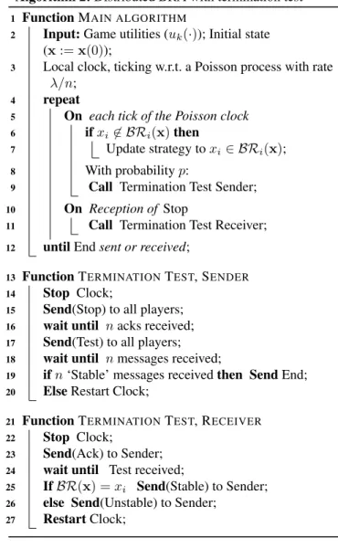
Under the Intersection Free Approximation, every time a new player who is not satisfied (in the algorithm, that correspond to a player not in L) has to compute its best response in
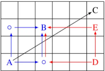
Roubens, Equivalent Representations of a Set Function with Applications to Game Theory and Multicriteria Decision Making, Preprint 9801, GEMME, Faculty of Economy, University of

In our experiment the control did not produce results in line with the theoretical expectations (Shapley value, or even a payoff allocation residing in the