HAL Id: hal-01856212
https://hal.inria.fr/hal-01856212v2
Submitted on 2 Mar 2020
HAL is a multi-disciplinary open access
archive for the deposit and dissemination of sci-entific research documents, whether they are pub-lished or not. The documents may come from
L’archive ouverte pluridisciplinaire HAL, est destinée au dépôt et à la diffusion de documents scientifiques de niveau recherche, publiés ou non, émanant des établissements d’enseignement et de
ExpectHill estimation, extreme risk and heavy tails
Abdelaati Daouia, Stephane Girard, Gilles Stupfler
To cite this version:
Abdelaati Daouia, Stephane Girard, Gilles Stupfler. ExpectHill estimation, extreme risk and heavy tails. Journal of Econometrics, Elsevier, 2021, 221 (1), pp.97-117. �10.1016/j.jeconom.2020.02.003�. �hal-01856212v2�
ExpectHill estimation, extreme risk and heavy tails
Abdelaati Daouiaa, St´ephane Girardb and Gilles Stupflerc
a Toulouse School of Economics, University of Toulouse Capitole, France b Univ. Grenoble Alpes, Inria, CNRS, Grenoble INP, LJK, France c Univ Rennes, Ensai, CNRS, CREST - UMR 9194, F-35000 Rennes, France
Abstract: Risk measures of a financial position are, from an empirical point of view, mainly based on quantiles. Replacing quantiles with their least squares analogues, called ex-pectiles, has recently received increasing attention. The novel expectile-based risk measures satisfy all coherence requirements. We revisit their extreme value estimation for heavy-tailed distributions. First, we estimate the underlying tail index via weighted combinations of top order statistics and asymmetric least squares estimates. The resulting expectHill estimators are then used as the basis for estimating tail expectiles and Expected Shortfall. The asymp-totic theory of the proposed estimators is provided, along with numerical simulations and applications to actuarial and financial data.
JEL Classifications: C13, C14.
Keywords: Asymmetric least squares, Coherent risk measures, Expected shortfall, Ex-pectile, Extrapolation, Extremes, Heavy tails, Tail index.
1
Introduction
The risk of a financial position Y is usually summarized by a risk measure. Value at Risk (VaR) is arguably the most common risk measure used in practice. The VaR at probability level τ P p0, 1q is given by the τ -quantile qτ :“ FYÐpτ q “ infty P R : F pyq ě τ u, where
F is the distribution function of Y . Koenker and Bassett [35] elaborated an absolute error loss minimization framework extending this definition of quantiles as left continuous inverse functions to the minimizers
qτ P arg min θPR E t%
τpY ´ θq ´ %τpY qu ,
with equality if F is increasing, where %τpyq “ |τ ´ 1Ipy ď 0q| |y| and 1Ip¨q is the indicator
function. There are different sign conventions for VaR which co-exist in the literature. In this paper, the position Y is a real-valued random variable whose values are the negative of financial returns. The right-tail of the distribution of Y , for levels τ close to one, then corresponds to the negative of extreme losses. In actuarial science where Y is typically a non-negative loss variable, the sign convention we have chosen implies that extreme losses also correspond to levels τ close to one. The position Y is therefore considered riskier as its risk measure gets higher.
One of the major criticisms on the VaR qτ is its failure to fulfill the subadditivity property
in general (Acerbi [1]), and hence it is not a coherent risk measure according to the axiomatic foundations in Artzner et al. [2]. Furthermore, it fails to account for the size of losses beyond the level τ , since quantiles only depend on the frequency of tail losses and not on their values (Dan´ıelsson et al. [12]). In both of these aspects, expectiles are a perfectly reasonable
alternative to quantiles as they depend on both the tail realizations and their probability (Kuan et al. [37]) and define a coherent risk measure for τ ě 12 (Bellini et al. [5]). This is mainly due to their conception as a least squares analogue of quantiles. More precisely, by substituting the absolute deviations in the asymmetric loss function %τ with squared
deviations, Newey and Powell [39] obtain the τ th expectile of the distribution of Y as the minimizer
ξτ :“ arg min θPR E tη
τpY ´ θq ´ ητpY qu , (1)
with ητpyq “ |τ ´ 1Ipy ď 0q| y2. The additional term ητpY q ensures the existence of a unique
solution ξτ for distributions with finite absolute first moment. Expectiles are determined by
tail expectations rather than tail probabilities, which allows for more prudent and reactive risk management. Altering the shape of extreme losses may not change the quantile-VaR, but it does impact all the expectiles (Taylor [45]). Another advantage of expectiles is that they make more efficient use of the available data since they rely on the distance to all ob-servations and not only on the frequency of tail losses (Sobotka and Kneib [44]). Moreover, using expectiles has the appeal of avoiding recourse to regularity conditions on the underlying distribution (see e.g. Holzmann and Klar [32], Kr¨atschmer and Z¨ahle [36]). Perhaps most importantly, expectiles induce the only coherent law-invariant risk measure that is elicitable (Ziegel [49]). The property of elicitability corresponds to the existence of a natural backtest-ing methodology. Also, expectiles are the only M-quantiles (Brecklbacktest-ing and Chambers [7]) that are coherent risk measures (Bellini et al. [5]). Further theoretical and numerical merits in favor of the adoption of expectiles in risk management can be found in Ehm et al. [21] and Bellini and Di Bernardino [6].
Expected Shortfall (ES). It is favored by practitioners who are more concerned with the risk exposure to a catastrophic event that may wipe out an investment in terms of the size of potential losses. The conventional quantile-based ES at level τ equals
QESτ :“ 1 1 ´ τ
ż1
τ
qtdt.
It is coherent (Acerbi [1]) and identical, when the financial position Y is continuous, to the so-called Conditional Value at Risk ErY |Y ą qτs (Rockafellar and Uryasev [42, 43]).
Similarly to this intuitive tail conditional expectation, Taylor [45] has introduced and used the expectile-based form ErY |Y ą ξτs as the basis for estimating the standard
quantile-based measure ErY |Y ą qτs. Given that both conditional expectations ErY |Y ą qτs and
ErY |Y ą ξτs are not coherent risk measures in general, Daouia et al. [15] have suggested to
estimate the coherent ES form QESτ on the basis of its expectile-based analogue
XESτ :“ 1 1 ´ τ ż1 τ ξtdt,
obtained by substituting the expectile ξtin place of the quantile qt in QESτ. This definition
is more convenient than ErY |Y ą ξτs as it induces a proper coherent risk measure (see
Proposition 2 in Daouia et al. [15]).
And yet, despite this substantial body of work on expectiles and their inference, the problem of estimating tail expectiles from the perspective of extreme value theory has been much less addressed. This translates into considering both intermediate and extreme asym-metry levels, respectively, τ “ τn Ñ 1 such that np1 ´ τnq Ñ 8 and τ “ τn1 Ñ 1 such that
np1 ´ τ1
max-imum domain of attraction of heavy-tailed distributions that describe the tail structure of most actuarial and financial data fairly well (see, e.g., Embrechts et al. [25] and Resnick [40]). This problem is, in comparison to extreme quantile estimation, still in full development. The absence of a closed form expression for expectiles makes the extreme value analysis of their asymmetric least squares estimators a much harder mathematical problem than for order statistics. Yet, we have initiated a satisfactory solution to this problem in Daouia et al. [13] by proposing intermediate and extreme expectile estimators and developing their asymptotic theory. Very recently, we have come up in Daouia et al. [15] with powerful approximations of the tail empirical expectile process. First, Theorem 1 in Daouia et al. [15] derives an ex-plicit joint asymptotic Gaussian representation of the tail expectile and quantile processes. Second, Theorem 2 in Daouia et al. [15] unravels the discrepancy between the tail empirical expectile process and its population counterpart. As these two theorems constitute the basic theoretical tools for our asymptotic analysis in the present paper, they are briefly described below in Proposition 1along with the statistical model in Section 2.
Let us now highlight the contribution of this paper, which is threefold. First, building on Proposition 1, Section 3 shows that the tail index of the underlying Pareto-type distri-bution can be estimated in a novel manner. This index tunes the tail heaviness of F and its knowledge is of utmost interest since it makes the estimation of extreme quantiles and expectiles possible by means of appropriate extrapolation techniques. We first construct asymmetric least squares estimators of the tail index and derive their asymptotic normality in Theorem1. We then construct a more general class of weighted estimators by computing a linear combination of these pure expectile-based estimators and of the popular Hill estimator (Hill [31]). This inspired the name expectHill estimators for this class. Thanks to the joint
weighted Gaussian approximations of the tail expectile and quantile processes in Proposi-tion1, we prove the asymptotic normality of the expectHill estimators and derive their joint convergence with both intermediate quantile and expectile estimators in Theorem 2.
Second, building on the expectHill estimators themselves, we propose in Section4general weighted estimators for intermediate expectiles ξτn whose asymptotic normality, obtained
in Theorem 3, follows as a corollary of Theorem 2. The weighted intermediate expectile estimators are then extrapolated to the very extreme expectile level τ1
n that may approach
one at an arbitrarily fast rate. The asymptotic properties of the extrapolated ξτ1
n estimators
are established in Theorem 4.
Third, we note that the proposed estimation procedures in Daouia et al. [15] for both extreme values XESτ1
n and QESτn1 are mainly based on the classical Hill estimator of the tail
index. In Section5, we extend their extrapolation devices by using the generalized weighted expectHill estimator; see Theorems 5-6.
In Section 6, we discuss the important issue of parameter selection in our weighted estimators. Section7contains our experiments with simulated data and Section8presents a concrete application to financial returns data. Section9 concludes. Proofs, auxiliary results and additional simulation results are deferred to the Supplementary Material document.
2
Statistical model and basic tools
In this paper we consider the class of heavy-tailed distributions, referred to as the Fr´echet maximum domain of attraction, with tail index 0 ă γ ă 1. The survival function of these
Pareto-type distributions has the form
F pyq :“ 1 ´ F pyq “ y´1{γ`pyq, (2)
for y ą 0 large enough, where ` is a slowly varying function at infinity, i.e., a positive function on p0, 8q satisfying `ptyq{`ptq Ñ 1, as t Ñ 8, for any y ą 0. The index γ tunes the tail heaviness of F : the larger the index, the heavier the right tail. Let Y be the actuarial or financial position of interest having survival function F , and let Y´ “ minpY, 0q denote
the negative part of Y . Then, together with condition E|Y´| ă 8, the assumption γ ă 1
ensures the existence of the first moment of Y , and hence the existence of expectiles. By Corollary 1.2.10 in de Haan and Ferreira [16], the model assumption (2) is equivalent to
lim
tÑ8
U ptxq U ptq “ x
γ for all x ą 0, (3)
where U ptq :“ q1´t´1 ” infty P R : 1{F pyq ě tu stands for the tail quantile function of Y .
Under (2) or equivalently (3), it has been found that
ξτ
qτ
„ pγ´1´ 1q´γ as τ Ñ 1 (4)
(Bellini and Di Bernardino [6]). A refined asymptotic expansion of ξτ{qτ with a precise
quantification of the error term is obtained in Mao et al. [38] under the following second-order regular variation condition:
C2pγ, ρ, Aq For all x ą 0, lim tÑ8 1 Aptq „ U ptxq U ptq ´ x γ “ xγx ρ ´ 1 ρ
where ρ ď 0 is a constant parameter and A is an auxiliary function converging to 0 at infinity and having ultimately constant sign. Hereafter, pxρ´ 1q{ρ is to be understood as log x when
ρ “ 0.
Assumption C2pγ, ρ, Aq is a standard condition in extreme value theory, which controls the
rate of convergence in (3). The monographs of Beirlant et al. [4, Section 3.3 and particularly 3.3.2, p.93] and de Haan and Ferreira [16, Section 2.3, p.43] give abundant examples of com-monly used continuous distributions satisfying C2pγ, ρ, Aq, along with thorough discussions
on the interpretation and the rationale behind this second-order condition. For instance, the (Generalized) Pareto, Burr, Fr´echet, Student, Fisher and Inverse-Gamma distributions all satisfy this condition, and more generally so does any distribution whose survival function has the form
1 ´ F pxq “ x´1{γ`a ` bx´c` opx´cq˘ as x Ñ 8,
where a ą 0, b P Rzt0u and c ą 0 are constants. This contains in particular the Hall-Weiss class of models (see Hua and Joe [33]), where condition C2pγ, ρ, Aq is met with ρ “ ´cγ and
Aptq “ ´a´cγ´1bcγ2t´cγ.
Suppose we observe independent copies tY1, . . . , Ynu of the random variable Y and denote
by Y1,nď Y2,nď ¨ ¨ ¨ ď Yn,n their nth order statistics. Let the expectile level τ “ τnapproach
of the corresponding intermediate expectile ξτn is given by its empirical version r ξτn “ arg min uPR n ÿ i“1 ητnpYi´ uq, (5)
where ητpyq “ |τ ´ 1Ipy ď 0q| y2. Under condition C2pγ, ρ, Aq, Daouia et al. [15] prove in their
Theorem 1 that the tail empirical expectile process
p0, 1s Ñ R, s ÞÑ rξ1´p1´τnqs
can be approximated by a sequence of Gaussian processes with drift and derive its joint asymptotic behavior with the tail empirical quantile process
p0, 1s Ñ R, s ÞÑ pq1´p1´τnqs :“ Yn´tnp1´τnqsu,n,
where t¨u stands for the floor function. They also analyze in their Theorem 2 the difference between the tail empirical expectile process and its population counterpart. For our purposes below, we recall these two approximations in the following result.
Proposition 1 (Daouia et al., 2020). Suppose that E|Y´|2 ă 8. Assume further that
condition C2pγ, ρ, Aq holds, with 0 ă γ ă 1{2. Let τn Ñ 1 be such that np1 ´ τnq Ñ 8 and
a
np1 ´ τnqApp1 ´ τnq´1q “ Op1q. Then there exists a sequence Wn of standard Brownian
processes involved, p q1´p1´τnqs qτn “ s´γ ˜ 1 ` a 1 np1 ´ τnq γaγ´1´ 1 s´1W n ˆ s γ´1´ 1 ˙ `s ´ρ ´ 1 ρ App1 ´ τnq ´1 q ` oP ˜ s´1{2´ε a np1 ´ τnq ¸¸ and ξr1´p1´τnqs ξτn “ s´γ ˆ 1 ` psγ´ 1qγpγ ´1´ 1qγ qτn pEpY q ` oPp1qq ` a 1 np1 ´ τnq γ2aγ´1´ 1 sγ´1 żs 0 Wnptq t´γ´1dt ` p1 ´ γqpγ ´1 ´ 1q´ρ 1 ´ γ ´ ρ ˆ s´ρ ´ 1 ρ App1 ´ τnq ´1 q ` oP ˜ s´1{2´ε a np1 ´ τnq ¸¸ uniformly in s P p0, 1s. If in addition ρ ă 0, then r ξ1´p1´τnqs ξ1´p1´τnqs “ 1 ` a 1 np1 ´ τnq γ2aγ´1´ 1 sγ´1 żs 0 Wnptq t´γ´1dt ` oP ˜ s´1{2´ε a np1 ´ τnq ¸ uniformly in s P p0, 1s.
The assumptions that γ P p0, 1{2q and E|Y´|2 ă 8 essentially guarantee that the loss
variable has a finite variance. This is the case in most studies on actuarial and financial data where the estimated values of γ have been found to lie below 1{2; see, e.g., the R package CASdatasets, Daouia et al. [13] and the references therein.
extrapolation results formulated in the extreme value literature under condition C2pγ, ρ, Aq;
see, e.g., Chapter 4 of de Haan and Ferreira [16] regarding extreme quantile estimation and Daouia et al. [13] for extreme expectile estimation. Note also that, in contrast to the first part of Proposition 1, the second part avoids the error terms that are proportional to 1{qτn
and App1 ´ τnq´1q.
This result, already proved in Daouia et al. [15], constitutes the main intermediate the-oretical tool for our ultimate interest in constructing general weighted estimators of the tail index and extreme expectiles, as well as of Expected Shortfall risk measures.
3
Estimation of the tail index
In this section, we first construct purely expectile-based estimators of the tail index γ and derive their asymptotic distributions. We shall then construct a more general class of esti-mators by combining both intermediate empirical expectiles and quantiles. The basic idea stems from Proposition 1 which suggests the following approximation:
ż1 0 log ˜ r ξ1´p1´τnqs ξτn ¸ ds « ż1 0 logps´γ q ds “ γ
where τn Ñ 1 is such that np1 ´ τnq Ñ 8. One can then estimate γ by
q γτn :“ ż1 0 log ˜ r ξ1´p1´τnqs r ξτn ¸ ds.
A computationally more viable option is to use a discretized version of the integral estimator q
γτn on a regular l´grid of points in r0, 1s, namely:
r γτn,l :“ 1 l l ÿ i“1 log ˜ r ξ1´p1´τnqpi´1q{l r ξτn ¸
where l “ lpnq Ñ 8. A particularly interesting example is
r γτn :“ 1 tnp1 ´ τnqu tnp1´τnqu ÿ i“1 log ˜ r ξ1´pi´1q{n r ξ1´tnp1´τnqu{n ¸ (6)
or, equivalently, rγτn “ rγ1´tnp1´τnqu{n,tnp1´τnqu. This simple estimator has exactly the same
form as the popular Hill estimator (Hill [31])
p γτn “ 1 tnp1 ´ τnqu tnp1´τnqu ÿ i“1 log ˆ p q1´pi´1q{n p q1´tnp1´τnqu{n ˙ (7)
with the tail empirical quantile process q in (p 7) replaced by its asymmetric least squares analogue rξ. Beirlant et al. [4] and de Haan and Ferreira [16] provide an extensive overview of the asymptotic theory for the Hill estimator pγτn. The next theorem gives the asymptotic
normality of the three new estimators qγτn, rγτn,l and rγτn. Its proof essentially consists in
writing log ˜ r ξ1´p1´τnqs r ξτn ¸ “ log ˜ r ξ1´p1´τnqs ξτn ¸ ´ log ˜ r ξτn ξτn ¸
before integrating and crucially using Proposition 1 twice in order to control both of the logarithms on the right-hand side.
with 0 ă γ ă 1{2. Let τn Ñ 1 be such that np1 ´ τnq Ñ 8, and suppose that the bias
conditions anp1 ´ τnqApp1 ´ τnq´1q Ñ λ1 P R and
a np1 ´ τnq{qτn Ñ λ2 P R are satisfied. Then: (i) anp1 ´ τnqpqγτn´ γq d ÝÑ N ˆ p1 ´ γqpγ´1´ 1q´ρ p1 ´ ρqp1 ´ γ ´ ρqλ1´ EpY q γ2pγ´1´ 1qγ γ ` 1 λ2, 2γ3 1 ´ 2γ ˙ .
(ii) If l “ lpnq fulfills anp1 ´ τnq logpnp1 ´ τnqq{l Ñ 0, then (i) holds with qγτn replaced by
r
γτn,l. Especially, (i) holds with qγτn replaced by rγτn.
Before using the estimatorrγτn to construct a more general class of tail index estimators,
we formulate a couple of remarks about its theoretical and practical behavior.
Remark 1. The conditions involving the auxiliary function A in Theorem 1 are also re-quired to derive the asymptotic normality of the conventional Hill estimatorγpτn in (7), with
asymptotic bias λ1{p1 ´ ρq and asymptotic variance γ2 [see Theorem 3.2.5 in de Haan and
Ferreira ([16], p.74)]. Theorem1also features a further bias condition involving the quantile function q; this was to be expected in view of Proposition 1, of which a consequence is that the remainder term in the approximation ξ1´p1´τnqs{ξτn « s
´γ depends on both A and q.
Remark 2. The selection of τn is a difficult problem in general, since any sort of
opti-mal choice will involve the unknown parameter ρ as well as the function A; for a discussion about the optimal choice of τnin the Hill estimator based on mean-squared error, see Hall and
Welsh [30]. A usual practice for selecting a reasonable estimate pγτn is, in the
pick out a value of k corresponding to the first stable part of the plot [see, e.g., de Haan and Ferreira ([16], Section 3)]. There have been a number of attempts at formalizing this procedure, including Resnick and St˘aric˘a [41], Drees et al. [20], and more recently El Methni and Stupfler [23, 24]. The Hill plot may be, however, so unstable that reasonable values of k (which would correspond to estimates close to the true value of γ) may be hidden in the graph. The least squares analogue rγ1´k{n in (6) is, in contrast to pγ1´k{n, based on ex-pectiles that enjoy superior regularity properties compared to quantiles (see Proposition 1 in Holzmann and Klar [32]). One may thus expect that rγ1´k{n affords smoother and more
stable plots compared to those of the Hill estimator pγ1´k{n. This advantage is illustrated in
Section A of the Supplementary Material document, where we examine the properties of pγ and rγ on real financial data. It can be seen thereon that the plots of k ÞÑrγ1´k{n are indeed far smoother than the arguably wiggly plots of k ÞÑpγ1´k{n.
It could, however, happen that rγ has a higher bias than the Hill estimator. This is for instance the case if |ρ| is large, since a large |ρ| means that the underlying distribution is, in its right tail, very close to a multiple of the Pareto distribution for which the Hill estimator is unbiased. A natural way to take advantage of the desirable properties of both rγ and pγ in a large class of models is by using their linear combination for estimating γ. For α P R, we then define the more general estimator
γτnpαq :“ αpγτn` p1 ´ αqγrτn. (8)
We shall call this linear combination the expectHill estimator. For example, the simple mean γτnp1{2q would represent an equal balance between the use of large asymmetric least squares
statistics in (6) and top order statistics in (7). The convergence of the expectHill estimator is, however, a highly non-trivial problem as it hinges, by construction, on both the tail expectile and quantile processes. The explicit joint asymptotic Gaussian representation of these two processes, obtained in Proposition 1, is a pivotal tool for our analysis, and enables us to address the convergence problem in its full generality. We establish below the asymptotic normality of the expectHill estimator, along with its joint convergence with intermediate sample quantiles and expectiles.
Theorem 2. Suppose that the conditions of Theorem 1 hold. Then, for any α P R,
a np1 ´ τnq ˜ γτnpαq ´ γ,qpτn qτn ´ 1,ξrτn ξτn ´ 1 ¸ d ÝÑ N pmα, Vαq
where mα is the 1 ˆ 3 vector mα :“ pbα, 0, 0q, with
bα “ λ1 1 ´ ρ ˆ α ` p1 ´ αqp1 ´ γqpγ ´1´ 1q´ρ 1 ´ γ ´ ρ ˙ ´ p1 ´ αqEpY qγ 2pγ´1´ 1qγ γ ` 1 λ2, (9) and Vα is the 3 ˆ 3 symmetric matrix with entries
Vαp1, 1q “ γ2 ˆ α2„ 3 ´ 4γ 1 ´ 2γ ´ 2 pγ´1´ 1qγ 1 ´ γ ´ 2α „ 1 1 ´ 2γ ´ pγ´1´ 1qγ 1 ´ γ ` 2γ 1 ´ 2γ ˙ , Vαp1, 2q “ p1 ´ αqγrpγ´1´ 1qγ´ 1 ´ γ logpγ´1´ 1qs, Vαp1, 3q “ γ3 p1 ´ γq2 „ αpγ´1 ´ 1qγ` p1 ´ αq 1 ´ γ 1 ´ 2γ , Vαp2, 2q “ γ2, Vαp2, 3q “ γ2 ˆ pγ´1´ 1qγ 1 ´ γ ´ 1 ˙ , Vαp3, 3q “ 2γ3 1 ´ 2γ.
As an immediate consequence, we have for any α P R, a
np1 ´ τnq`γτnpαq ´ γ
˘ d
ÝÑ N pbα, vαq where vα “ Vαp1, 1q. (10)
This remains valid if rγτn is replaced in (8) by the continuous version qγτn, or any other
discretized version rγτn,l provided
a
np1 ´ τnq logpnp1 ´ τnqq{l Ñ 0.
In this situation where the estimator γτnpαq depends on a weighting parameter α P R, a reasonable question is to seek the value(s) (if any) of the parameter α giving in some sense the “best” performing estimator in the class pγτnpαqqαPR. A standard measure of the
quality of the estimator is the Asymptotic Mean-Squared Error (AMSE). Minimizing this quantity for the estimator γτnpαq would amount to minimizing the quantity b2α ` vα with
respect to α. This is a degree 2 convex polynomial in α, and therefore this minimization is theoretically completely straightforward. In practice though, computing the value of the optimal α˚ minimizing this AMSE requires the knowledge of ρ, λ
1, λ2, γ and EpY q. The
accurate estimation of the particular quantities ρ and λ1 is known to be difficult to implement
in practice and requires involved methodologies, see e.g. the Introduction of [8]. In contrast to the sum b2
α ` vα, the calculation of the single asymptotic variance term vα, which also
defines a degree 2 convex polynomial in α, requires only the estimation of the parameter γ for which we can simply plug in, for instance, the Hill estimator already in use. Focusing on the minimization of the variance term vα and ignoring the bias term bα may therefore be a
plausible pragmatic strategy. We expand upon this choice of the parameter α in our next remark.
variance vα of γτnpαq, only depends on the tail index γ and has the explicit expression
αpγq “ p1 ´ γq ´ p1 ´ 2γqpγ
´1
´ 1qγ p1 ´ γqp3 ´ 4γq ´ 2p1 ´ 2γqpγ´1´ 1qγ.
Its plot against γ P p0, 1{2q is given in Figure 1(a). Interestingly, this optimal value of α is negative for small values of γ, say γ ď 0.2. By contrast, for large values of γ (close to 1{2), it tends to one, favoring thus the robustness of order statistics over the tail sensitivity of asymmetric least squares. In the special case of stock returns, where realized values of the tail index were found in Gabaix [26] to be γ « 1{3, the corresponding variance-optimal combination parameter αpγq varies around αp1{3q « 0.9. It can also be seen that the simple mean γτnp1{2q of pγτn and γrτn, with α “ 1{2, minimizes the asymptotic variance vα for
γ “ 1{4. This is unsurprising since both γpτn and rγτn have the same asymptotic variance
in this case, as illustrated in Figure 2 in the Supplementary Material document. It can be seen thereon that the simple mean γτnp1{2q affords a middle course between pγτn ” γτnp1q
and rγτn ” γτnp0q in terms of asymptotic variance. In terms of smoothness, γτnp1{2q offers a
middle course as well, as shown in Section A of the Supplementary Material document.
Remark 4. Let us comment on the covariance of pγτn and rγτn, as well as the variance of the
expectHill estimator given by
Vpγτnpαqq “ α
2
Vppγτnq ` p1 ´ αq
2
Vprγτnq ` 2αp1 ´ αqCovppγτn,rγτnq.
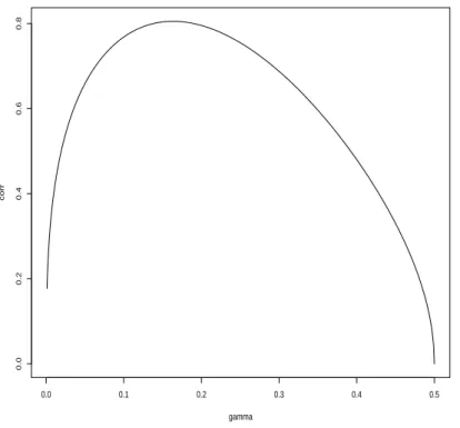
docu-0.0 0.4 0.8 0.0 0.1 0.2 0.3 0.4 0.5 gamma O pt ima l va lu e o f al ph a (a) 0.0 0.3 0.6 0.9 0.0 0.1 0.2 0.3 0.4 0.5 gamma O pt ima l va lu e o f be ta (b)
Figure 1: (a) — Evolution of the variance-optimal value αpγq against γ P p0, 1{2q. The dotted lines represent the values α “ 0 and α “ 1. (b) — Evolution of the variance-optimal value βαpγqpγq against γ P p0, 1{2q. The dotted lines represent the values β “ 0 and β “ 1.
ment) reveals that the asymptotic covariance ofpγτn and γrτn is
Covppγτn,rγτnq “ γrpγ ´1 ´ 1qγ´1´ γs “ γ2 ˆ pγ´1´ 1qγ 1 ´ γ ´ 1 ˙ . Since Vppγτnq “ γ 2 and Vprγ τnq “ 2γ 3
correlation term corrppγτn,rγτnq “ Covppγτn,rγτnq a VppγτnqVprγτnq “c 1 ´ 2γ 2γ ˆ pγ´1´ 1qγ 1 ´ γ ´ 1 ˙ .
This correlation as a function of γ P p0, 1{2s is represented on Figure 2. It seems to be a concave function of γ, attaining a maximum of approximately 0.8 at around γ “ 1{6. Note though that for α “ 1{2 and γ “ 1{6, we have Vpγτnpαqq{Vppγτnq « 2{3. Consequently, even
for values of γ where the correlation between pγτn and γrτn is high, the improvement brought
in terms of variance by considering the expectHill estimator can be very substantial.
0.0 0.1 0.2 0.3 0.4 0.5 0.0 0.2 0.4 0.6 0.8 gamma corr
4
Extreme expectile estimation
In this section, we first return to intermediate expectile estimation by making use of the general class of γ estimators tγτnpαquαPR to construct alternative estimators for high
expec-tiles ξτn such that τnÑ 1 and np1 ´ τnq Ñ 8 as n Ñ 8. Then we extrapolate the obtained
estimators to the very high expectile levels that may approach one at an arbitrarily fast rate. Alternatively to the asymmetric least squares estimator rξτn defined in (5), one may use
the asymptotic connection ξτn „ pγ
´1 ´ 1q´γq
τn, described in (4), to define the following
semiparametric estimator of ξτn: p ξτnpαq :“`γτnpαq ´1 ´ 1˘´γτnpαq p qτn.
In the special case α “ 1, we recover the purely quantile-based estimator pξτnp1q suggested
in Daouia et al. [13]. The asymmetric least squares estimator rξτn inherits the requisite
property of coherency of the true risk measure ξτn and is superior to pξτnp1q in terms of
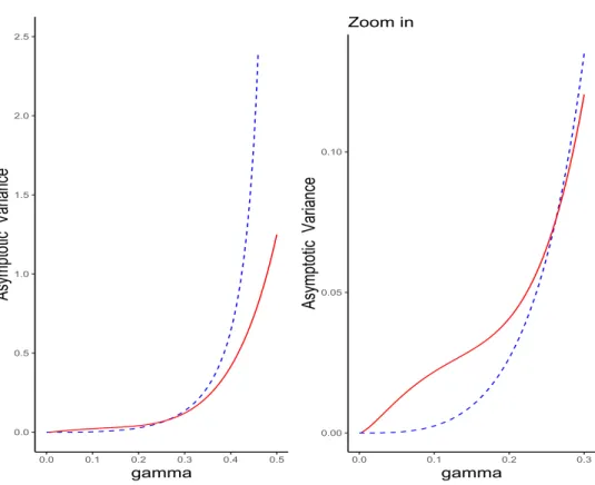
asymptotic variance when the tail index γ ă 0.3, as visualized in Figure3(right-hand side). By contrast, pξτnp1q is more efficient over the range of values of γ ą 0.3 that are common
in actuarial and financial applications, as can be seen from Figure 3 (left-hand side). The asymptotic variances of both rξτn and pξτnp1q can be found in Daouia et al. [13] and follow as
special cases from Theorem 3below.
In order to obtain the best of both pξτnp1q and rξτn, it is then natural to consider their
0.0 0.5 1.0 1.5 2.0 2.5 0.0 0.1 0.2 0.3 0.4 0.5 gamma Asymp to tic Va ria nce 0.00 0.05 0.10 0.0 0.1 0.2 0.3 gamma Asymp to tic Va ria nce Zoom in
Figure 3: Asymptotic variances of rξτn in dashed blue line and pξτnp1q in solid red line, with
γ P p0, 1{2q.
to define, for β P R, the weighted estimator
ξτnpα, βq :“ β pξτnpαq ` p1 ´ βq rξτn. (11)
When α “ 1, we recover the particular expectile estimator ξτnpβq :“ ξτnp1, βq introduced
in Daouia et al. [15]. The limit distribution of the more general variant ξτnpα, βq crucially relies on the asymptotic dependence structure in Theorem 2 between γτnpαq, qpτn and rξτn.
Theorem 3. Suppose that the conditions of Theorem 1 hold. Then, for any α, β P R, a np1 ´ τnq ˜ ξτnpα, βq ξτn ´ 1 ¸ d ÝÑ β`bα` rp1 ´ γq´1´ logpγ´1´ 1qsΨα` Θ ˘ ` p1 ´ βqΞ
where the bias component bα is bα “ λ1b1,α` λ2b2,α with
b1,α “ p1 ´ γq´1´ logpγ´1´ 1q 1 ´ ρ „ α ` p1 ´ αqp1 ´ γqpγ ´1 ´ 1q´ρ 1 ´ γ ´ ρ ´ pγ ´1 ´ 1q´ρ 1 ´ γ ´ ρ ´ pγ´1´ 1q´ρ´ 1 ρ , b2,α “ ´γpγ´1´ 1qγEpY q ˆ 1 ` p1 ´ αqrp1 ´ γq´1 ´ logpγ´1´ 1qs γ γ ` 1 ˙ ,
and pΨα, Θ, Ξq is a trivariate Gaussian centered random vector with covariance matrix Vα
as in Theorem 2.
Similarly to the tail index estimator γτnpαq, the expectile estimator
ξτnpα, βq ” β `γτnpαq
´1
´ 1˘´γτnpαq
p
qτn ` p1 ´ βq rξτn
depends on a weighting parameter pα, βq P R2. The optimal value pα˚, β˚q minimizing the
AMSE of ξτnpα, βq is also difficult to estimate, as it depends on the elusive parameters ρ and λ1. Our strategy here will thus be to set first α “ αpγq, the variance-optimal choice of
the weighting parameter in the estimator γτnpαq at the heart of the construction of ξτnpα, βq,
and then to determine the parameter β minimizing the asymptotic variance of ξτnpαpγq, βq. This is a sensible approach to find a low-variance estimator within the class pξτnpα, βqqpα,βqPR2.
es-timator γτnpαq in (8) [see Remark 3], the combination parameter β, which minimizes the asymptotic variance of the intermediate expectile estimator ξτnpα, βq in (11), has a closed form expression that only depends on the tail index γ. Indeed, this optimal value of β is obtained by minimizing the variance of the random quantity
β`rp1 ´ γq´1´ logpγ´1´ 1qsΨα` Θ
˘
` p1 ´ βqΞ,
where pΨα, Θ, Ξq is a trivariate Gaussian centered random vector with the covariance matrix
Vα given in Theorem2. Setting
mpγq :“ p1 ´ γq´1
´ logpγ´1´ 1q,
the above random quantity equals β pmpγqΨα` Θ ´ Ξq ` Ξ. Its variance is then
β2Var pmpγqΨα` Θ ´ Ξq ` 2β Cov pmpγqΨα` Θ ´ Ξ, Ξq ` Var Ξ.
The minimizer βαpγq of this variance is
βαpγq “ ´
Cov pmpγqΨα` Θ ´ Ξ, Ξq
Var pmpγqΨα` Θ ´ Ξq
, (12)
where the numerator can be rewritten explicitly as
and the denominator as
Var pmpγqΨα` Θ ´ Ξq “ rmpγqs2Vαp1, 1q ` Vαp2, 2q ` Vαp3, 3q
` 2mpγqVαp1, 2q ´ 2mpγqVαp1, 3q ´ 2Vαp2, 3q.
Taking the variance-optimal weight α ” αpγq in the expectHill estimator γτnpαq, the plot of the resulting variance-optimal value βαpγq ” βαpγqpγq against γ P p0, 1{2q is graphed in
Figure1(b). Interestingly, this quantity exceeds one for large values of γ, say γ ě 0.31. Let us now extend the estimation procedure far into the right tail, where few or no observations are available. This translates into considering the expectile level τ “ τ1
n Ñ 1
such that np1 ´ τ1
nq Ñ c P r0, 8q, as n Ñ 8. To estimate the extreme expectile ξτ1
n, the basic
idea is to extrapolate a consistent expectile estimator of intermediate order τn to the very
high level τ1
n. To do so, note that on the one hand we have ξτ1
n{ξτn „ qτn1{qτn in view of (4).
On the other hand, we have the classical Weissman extrapolation formula
qτ1 n qτn “ U pp1 ´ τ 1 nq´1q U pp1 ´ τnq´1q «ˆ 1 ´ τ 1 n 1 ´ τn ˙´γ
as τn and τn1 approach one (Weissman [48]). Thus, we arrive at the expectile approximation
ξτ1 n « ˆ 1 ´ τ1 n 1 ´ τn ˙´γ ξτn. (13)
By substituting our expectHill estimator γτnpαq and the general weighted intermediate es-timator ξτnpα, βq, respectively, in place of γ and ξτn, we get the extrapolated expectile
estimator ξ‹τ1 npα, βq :“ ˆ 1 ´ τ1 n 1 ´ τn ˙´γτnpαq ξτnpα, βq. (14) The special case α “ 1 corresponds to the estimator ξ‹τ1
npβq :“ ξ
‹ τ1
np1, βq introduced by
Daouia et al. [15]. We extend this estimator by using the generalized expectHill estimator γτnpαq instead of the Hill estimatorpγτn. The next theorem gives the asymptotic behavior of
ξ‹τ1
npα, βq.
Theorem 4. Suppose that the conditions of Theorem 1 hold. Assume also that ρ ă 0 and np1 ´ τ1
nq Ñ c ă 8 with
a
np1 ´ τnq{ logrp1 ´ τnq{p1 ´ τn1qs Ñ 8. Then, for any α, β P R,
a np1 ´ τnq logrp1 ´ τnq{p1 ´ τn1qs ˜ ξ‹τ1 npα, βq ξτ1 n ´ 1 ¸ d ÝÑ N pbα, vαq with pbα, vαq as in (9) and (10).
One can observe that the limiting distribution of ξ‹τ1
npα, βq is controlled by the asymptotic
distribution of γτnpαq. This is a consequence of the fact that the convergence of ξ‹τ1
npα, βq is
governed by that of the extrapolation factor rp1´τ1
nq{p1´τnqs´γτnpαq. The latter approximates
the theoretical factor rp1 ´ τ1
nq{p1 ´ τnqs´γ in the extrapolation (13) at a slower rate than
both the speed of convergence of ξτnpα, βq to ξτn, given by Theorem 3, and the speed of
convergence to 0 of the bias term that is incurred by the use of (13) and that can be controlled by Proposition 1.
5
Estimation of tail Expected Shortfall
This section aims to estimate both expectile- and quantile-based forms of Expected Shortfall,
XESτ :“ 1 1 ´ τ ż1 τ ξtdt, QESτ :“ 1 1 ´ τ ż1 τ qtdt, (15)
at a very extreme security level τ that may approach one at an arbitrarily fast rate. To do so, Daouia et al. [15] have already suggested to start by estimating these risk measures at an intermediate level τn Ñ 1 such that np1 ´ τnq Ñ 8, before extrapolating the resulting
estimates to the far tail by making use of the traditional Hill estimatorpγτn of the tail index γ.
Here, we extend their device by using the generalized expectHill estimator γτnpαq in place of p
γτn. The following asymptotic connections, established in Proposition 3 of Daouia et al. [15],
will prove instrumental in the estimation procedure.
Proposition 2 (Daouia et al., 2020). Assume that E|Y´| ă 8 and that Y has a Pareto-type
distribution (2) with tail index 0 ă γ ă 1. Then
XESτ QESτ „ ξτ qτ „ ErY |Y ą ξτs ErY |Y ą qτs and XESτ ξτ „ 1 1 ´ γ „ ErY |Y ą ξτs ξτ , τ Ñ 1.
5.1
Expectile-based Expected Shortfall
Under the model assumptions that E|Y´| ă 8 and Y has a heavy-tailed distribution (2),
we wish to estimate an extreme value of the expectile-based form XESτ1
n, where τ 1 n Ñ 1 and np1 ´ τ1 nq Ñ c ă 8. By Proposition2, we have XESτ1 n XESτ „ ξτ 1 n ξτ as n Ñ 8.
It follows from the approximation (13) that XESτ1 n « ´ 1´τ1 n 1´τn ¯´γ
XESτn. Then, by replacing
γ with γτnpαq and XESτn with its empirical counterpart
Ć XESτn :“ 1 1 ´ τn ż1 τn r ξtdt,
we obtain the extrapolated XESτ1
n estimator Ć XES‹τ1 npαq :“ ˆ 1 ´ τ1 n 1 ´ τn ˙´γτnpαq Ć XESτn. (16)
One may also estimate XESτ1
n by using the asymptotic equivalence XESτn1 „ p1 ´ γq
´1ξ τ1
n
in Proposition 2. By substituting γ and ξτ1
n with their estimators γτnpαq and ξ
‹ τ1
npα, βq,
described respectively in (8) and (14), we define the alternative XESτ1
n estimator XES‹τ1 npα, βq :“ r1 ´ γτnpαqs ´1ξ‹ τ1 npα, βq (17)
for the weights α, β P R. The next result provides the convergence of the two competing estimators ĆXES‹τ1
npαq and XES
‹ τ1
npα, βq of XESτn1.
Theorem 5. Assume that the conditions of Theorem 4 hold. Then, for any α, β P R,
a np1 ´ τnq logrp1 ´ τnq{p1 ´ τn1qs ˜ Ć XES‹τ1 npαq XESτ1 n ´ 1 ¸ d ÝÑ N pbα, vαq, and a np1 ´ τnq logrp1 ´ τnq{p1 ´ τn1qs ˜ XES‹τ1 npα, βq XESτ1 n ´ 1 ¸ d ÝÑ N pbα, vαq, with pbα, vαq as in (9) and (10).
The two estimators share the same asymptotic behavior from a theoretical point of view. However, our experience with simulated data in Section 7.3 indicates that ĆXES‹τ1
npαq tends
to be more efficient in the case of real-valued profit-loss distributions with heavy left and right tails, while XES‹τ1
npα, βq affords advantageous estimates in the case of non-negative
heavy-tailed loss distributions.
5.2
Quantile-based Expected Shortfall
In this section, we return to the estimation of the usual form QESpn of tail Expected Short-fall, for a pre-specified tail probability pn Ñ 1 with np1 ´ pnq Ñ c ă 8. We wish to
de-rive composite expectile-based estimators from the two XESτ1
n estimators introduced above,
where τ1
n “ τn1ppnq is to be determined. The starting point is the asymptotic equivalences
QESpn „ ErY |Y ą qpns and XESτn1 „ ErY |Y ą ξτn1s in Proposition2. The basic idea is then
to pick out τ1
n so that ξτ1
n ” qpn, and hence QESpn „ XESτn1. In this way, QESpn inherits the
extreme value estimators of XESτ1
n itself, namely ĆXES
‹ τ1 npαq in (16) and XES ‹ τ1 npα, βq in (17).
Yet, it remains to estimate the extreme expectile level τ1
nppnq :“ τn1 such that ξτ1
n “ qpn. It
has been found in Proposition 3 of Daouia et al. [13] that such a level satisfies
1 ´ τ1
nppnq „ p1 ´ pnq
γ
1 ´ γ as n Ñ 8,
under the model assumption of heavy tails (2) with tail index 0 ă γ ă 1. Built on our novel expectHill estimator γτnpαq of γ, we can then estimate τn1ppnq by
p τ1 nppnq :“ 1 ´ p1 ´ pnq γτ npαq 1 ´ γτnpαq. (18)
By substituting this estimated value in place of τ1
nppnq ” τn1 in the extrapolated
estima-tors ĆXES‹τ1
npαq and XES
‹ τ1
npα, βq, we obtain composite estimators that estimate XESτn1ppnq „
QESpn. The asymptotic properties of ĆXES‹τ1
npαq and XES
‹ τ1
npα, βq, stated in Theorem 5, still
hold true for their composite versions as estimators of QESpn, with the same conditions. Theorem 6. Suppose the conditions of Theorem 4 hold with pn in place of τn1. Then, for
any α, β P R, a np1 ´ τnq logrp1 ´ τnq{p1 ´ pnqs ˜ Ć XES‹ p τ1 nppnqpαq QESpn ´ 1 ¸ d ÝÑ N pbα, vαq, and a np1 ´ τnq logrp1 ´ τnq{p1 ´ pnqs ˜ XES‹ p τ1 nppnqpα, βq QESpn ´ 1 ¸ d ÝÑ N pbα, vαq, with pbα, vαq as in (9) and (10).
6
Selection of the weights
Since the seminal works of Crane and Crotty [11] and Bates and Granger [3], combining estimators or forecasts has come to be viewed as a simple and effective way to improve and robustify the estimation or forecasting accuracy over that offered by individual models. Two extensive reviews of the literature, techniques and applications of forecast combinations are Clemen [10] and Timmermann [46], see also Weiss et al. [47] for a recent survey. An important step beyond designing the individual competing estimators and their combination is how to weight them, or equivalently, how to assign in our setup appropriate values to the combination parameters α in the expectHill estimator γτnpαq and β in the intermediate expectile estimator ξτnpα, βq, described respectively in (8) and (11). One way to address
this issue is by setting α to be a suitable estimate of the weight αpγq that minimizes the asymptotic variance of γτnpαq. Given that αpγq has a closed form expression that only depends on γ itself (see Remark 3), this suggests using the following two-step estimation procedure:
• In a first step, one may estimate γ by the hybrid version γτnp12q “ rpγτn `rγτns{2, for
α “ 12. Any convex combination would have sufficed at this preliminary stage, but we do not see any reason to bias γτnpαq one way or the other;
• In a second step, one may use the consistent estimator ατn :“ αpγτnp
1
2qq of αpγq as the
desired combination parameter α in the expectHill estimator γτnpαq, resulting in
γτn :“ γτnpατnq, with γτnpαq “ αpγτn ` p1 ´ αqrγτn. (19)
Section 7.1 provides Monte Carlo evidence that the finite-sample performance of the two-step estimator γτn is quite remarkable in comparison with the best (in terms of asymptotic variance) version γτnpαpγqq that is calculated with the true variance-optimal weight αpγq itself. Section8shows how these practical guidelines can easily be implemented and applied through empirical data.
Let us now turn to the choice of the second combination parameter β in the intermediate expectile estimator ξτnpα, βq and other related expectile and expected shortfall estimators. Once the first combination parameter α is chosen as the optimal value αpγq that minimizes the asymptotic variance of the expectHill estimator γτnpαq, the second weight β can similarly be set as the optimal value βαpγq which minimizes the asymptotic variance of ξτnpα, βq,
Remark 5, motivates the plug-in estimator
βτn :“ βατnpγτnq, (20)
obtained by substituting the estimated values ατn and γτn in place of the population values
αpγq and γ.
When it comes to compute the intermediate expectile estimator ξτnpα, βq in (11), which is in turn used to compute the extreme expectile and expected shortfall estimators ξ‹τ1
npα, βq in (14), ĆXES‹τ1 npαq in (16), XES ‹ τ1 npα, βq in (17), and ĆXES ‹ p τ1 nppnqpαq and XES ‹ p τ1 nppnqpα, βq in
Theorem 6, we can consider using the following two-step procedure:
• First, estimate the combination parameters α and β by ατn and βτn, respectively;
• Second, use the tail expectile and expected shortfall estimators above, as if α and β were known, by substituting in the estimated values ατn and βτn.
Our experiments with simulated data in Sections 7.2-7.4 provide Monte Carlo evidence that the resulting two-step estimators perform remarkably well compared with their corresponding variance-optimal versions using the theoretical weights α “ αpγq and β “ βαpγqpγq.
Remark 6. From the theoretical standpoint, in view of the consistency of γτn in Theorem2
and the continuous dependence of αpγq and βαpγqpγq viewed as functions of γ, it is
straight-forward to show that the adaptive estimator γτnpατnq has the same asymptotic distribution
as γτnpαpγqq. Indeed
and therefore, under the conditions of Theorem2, γτnpατnq ´ γτnpαpγqq “ oPp1{
a
np1 ´ τnqq,
by the consistency of ατn and the
a
np1 ´ τnq´asymptotic normality of both pγτn and rγτn
stated in Theorem1. Similarly, the adaptive estimator ξτnpατn, βτnq has the same asymptotic
distribution as ξτnpαpγq, βαpγqpγqq.
7
Numerical simulations
In order to illustrate the behavior of the presented estimation procedures of the tail in-dex γ and the two expected shortfall forms XESτ1
n and QESpn, we consider the Student
t-distribution with 1{γ degrees of freedom, the Fr´echet distribution F pxq “ e´x´1{γ, x ą 0,
and the Pareto distribution F pxq “ 1 ´ x´1{γ, x ą 1. The finite-sample performance of the
different estimators is evaluated through their relative Mean-Squared Error (MSE) and bias, computed over 200 replications. All the experiments have sample size n “ 2,500 and true tail index γ P t0.33, 0.48u (motivated by a number of actuarial and financial applications where the realized values of γ were found to vary between 0.33 and 0.48, see Gabaix [26] for a nice survey and Cai et al. [9] and Daouia et al. [13] for very recent applications). In our estimators we used the extreme levels τ1
n“ pn “ 1 ´ 1{n and the intermediate level τn“ 1 ´ k{n, where
the integer k can be viewed as the effective sample size for tail extrapolation. To save space, all figures illustrating our simulation results are deferred to Section B of the Supplementary Material document.
7.1
Tail index estimation
We investigated the finite-sample performance of the two-step expectHill estimator γτn of the tail index γ, obtained in (19) by substituting in the estimate ατn “ αpγτnp
1
2qq of the
theoretical optimal weight αpγq described in Remark 3. As a first benchmark, we used the ‘variance-optimal’ expectHill version γτnpαpγqq that is defined in (8) in the same way as γτn, but calculated with the true weight αpγq itself (rather than its estimate ατn). A second
benchmark is the ‘hybrid’ expectHill estimator γτnp1{2q obtained with the average weight α “ 1{2. The last and most important benchmark is the ‘oracle’ expectHill estimator γτnpαq
obtained by selecting the value of α which minimizes its MSE. Remarkably, the Monte Carlo estimates, obtained in Supplement B.1, indicate that both ‘oracle’ and ‘variance-optimal’ expectHill estimators have very close MSE in all cases, which is good news for our variance-optimal selection device (though the oracle procedure may provide slightly better estimates, in terms of bias, for large values of γ). Moreover, in terms of both bias and MSE, the Monte Carlo estimates indicate that the accuracy of the two-step expectHill estimator γτn is quite respectable in comparison with the theoretical version γτnpαpγqq. Finally, while the ‘hybrid’ expectHill estimator γτnp1{2q performs quite well in the Student scenario, it is clearly outperformed by our two-step estimator γτn in both Fr´echet and Pareto scenarios.
7.2
Extreme expectile estimation
The simulation experiments undertaken here are concerned with the two-step estimator
ξ‹τ1 n :“ ξ ‹ τ1 npα, βq “ ˆ 1 ´ τ1 n 1 ´ τn ˙´γτnpαq ξτnpα, βq (21)
of the extreme expectile ξτ1
n. It is computed by substituting in the estimated values α “ ατn
and β “ βτn of the theoretical variance-optimal weights αpγq and βαpγqpγq, as described
in Section 6. Its accuracy is evaluated in comparison with the variance-optimal version ξ‹τ1
npαpγq, βαpγqpγqq itself that is obtained by replacing the combination parameters α and β
with the theoretical values αpγq and βαpγqpγq. We also considered two additional benchmark
estimators: the ‘hybrid’ version corresponding to the average weights α “ β “ 1{2, and the ‘oracle’ version obtained by selecting the values of α and β which minimize the MSE estimates. The Monte Carlo results we obtained in Supplement B.2 show that the use of the estimated values α “ ατn and β “ βτn provides, in all cases, very similar results, in terms
of both MSE and bias, to the variance-optimal weights αpγq and βαpγqpγq themselves. Most
importantly, the MSE and bias estimates based on our variance-optimal selection of weights appear to be quite good in comparison with the oracle estimates. Finally, although the hybrid version ξ‹τ1
np1{2, 1{2q exhibits a slightly better bias relative to the variance-optimal
estimates, the latter are superior in terms of MSE.
7.3
Expected shortfall XES
τ1n
estimation
We also compared the finite-sample performance of the two-step XESτ1
n estimators Ć XES‹τ1 n :“ ĆXES ‹ τ1 npαq “ ˆ 1 ´ τ1 n 1 ´ τn ˙´γτnpαq Ć XESτn, (22) XES‹τ1 n :“ XES ‹ τ1 npα, βq “ r1 ´ γτnpαqs ´1ξ‹ τ1 npα, βq (23)
that are computed by substituting in the estimated values α “ ατn and β “ βτn of the
benchmark versions ĆXES‹τ1
npαpγqq and XES
‹ τ1
npαpγq, βαpγqpγqq that are obtained by
substitut-ing in the variance-optimal weights α “ αpγq and β “ βαpγqpγq. The Monte Carlo estimates
of MSE and bias, obtained in Supplement B.3, indicate that the two-step estimators are very accurate with respect to their variance-optimal versions in all cases. Also, the estimates Ć
XES‹τ1
n seem to perform better in the case of the real-valued Student distribution, while their
competitors XES‹τ1
n appear to be the most efficient in the case of the non-negative Fr´echet
and Pareto distributions. It should be noted that the central part and the left tail of the underlying distribution have an impact on the behavior of the expectile-based estimators at the right tail. This effect would not occur in the case of pure quantile-based estimators that correspond to the combination weights α “ β “ 1. The reason for this is that quantiles only depend on the frequency of tail observations. By contrast, expectiles (for any asymmetry level τ ) rely on the distance to “all” observations due to their L2-nature. Accordingly,
shift-ing mass in the lower tail of a distribution has no impact on the quantiles of the upper tail, but it does have an impact on all the expectiles.
7.4
Expected shortfall QES
pnestimation
We have also undertaken simulation experiments to evaluate the finite-sample performance of the composite expectile-based estimators
Ć XES‹ p τ1 nppnq:“ ĆXES ‹ p τ1 nppnqpαq “ ˆ 1 ´pτ1 nppnq 1 ´ τn ˙´γτnpαq Ć XESτn (24) “ ˆ γτnpαq 1 ´ γτnpαq ˙´γτnpαq Ć XES‹pnpαq, XES‹ p τ1 nppnq :“ XES ‹ p τ1 nppnqpα, βq “ r1 ´ γτnpαqs ´1ξ‹ p τ1 nppnqpα, βq (25) “ ˆ γτ npαq 1 ´ γτnpαq ˙´γτnpαq XES‹pnpα, βq, where τp1
nppnq is defined in (18), with α “ ατn and β “ βτn. Note that, in view of
Proposi-tion 2 and (4), we have QESpn „ pγ´1´ 1qγXESpn, as n Ñ 8. Then, by replacing in this
asymptotic equivalence γ and XESpnwith their respective estimators γτnpαq and ĆXES
‹
pnpαq or
XES‹pnpα, βq, we get directly the composite estimators in (24) and (25). The latter estimate the same conventional expected shortfall QESpn as the purely quantile-based estimator
z QES‹pn :“ˆ 1 ´ pn 1 ´ τn ˙´pγτn 1 tnp1 ´ τnqu tnp1´τnqu ÿ i“1 Yn´i`1,n (26)
proposed by El Methni et al. [22]. We compared their MSE and bias in Supplement B.4 with those of zQES‹pn and those of their benchmark versions that are obtained with α “ αpγq and β “ βαpγqpγq. We arrive at the following tentative conclusions:
• In the case of the (real-valued) Student distribution, the best estimator is clearly Ć
XES‹
p τ1
• In the cases of Fr´echet and Pareto distributions (both positive), the other composite expectile-based estimator XES‹
p τ1
nppnq seems to be the winner.
8
Financial returns data
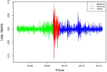
This section applies our expectHill-based method to estimate the tail expected shortfall on financial returns data. We use the same trade data as in the study of Kim and Meddahi [34] on the SPDR S&P 500 ETF (SPY), which is an exchange traded fund (ETF) that tracks the S&P 500 index. The dataset comprises 10 years of trade data on SPY starting from June 15th, 2004, to June 13th, 2014. The choice of the frequency of data, trading days and time horizon follows the same setup as in Kim and Meddahi [34]. This results in 2,497 days of trade data. Our sample consists of the negative returns pYiq depicted on Figure 4.
2006 2008 2010 2012 2014 -0 .1 0 -0 .0 5 0.00 0.05 0.10 Time Lo ss re tu rn s Before During After
Figure 4: Daily open-to-close loss returns (i.e. minus returns) of the SPDR S&P 500 ETF (SPY) starting from June 15th, 2004, to June 13th, 2014.
We use our composite expectile-based method to estimate the standard quantile-based ex-pected shortfall QESpn, or equivalently the expectile-based expected shortfall XESτ1
nppnq, with
an extreme relative frequency pn“ 1 ´ n1 that corresponds to a once-per-decade rare event.
The competing estimates ĆXES‹
p τ1 nppnq :“ ĆXES ‹ p τ1 nppnqpαq in (24) and XES ‹ p τ1 nppnq :“ XES ‹ p τ1 nppnqpα, βq
in (25) of QESpn are determined in two steps. We first choose the most favorable values of the weighting coefficients α and β, then we select an appropriate intermediate level τn for
each estimator. A common practice in extreme value analysis is to use the discrete reparam-eterization τn “ 1 ´ k{n, for the selected range of values 1 ď k ď n{ log n, where the integer
to be selected k represents the effective sample size for tail extrapolation.
First, we verify the model assumption of a heavy-tailed distribution with γ ă 12 that is required for the procedure. This assumption is already confirmed by the plots of the expectHill estimator γ1´k{npαq in Figure 1(a) in Section A of the Supplementary Material document, for the special cases α “ 0, 12, 1. The estimated values of γ obtained therein in Table 1 (second row) vary between γ1´k{np0q “ 0.33 and γ1´k{np1q “ 0.35, with γ1´k{np
1 2q “
0.34.
The optimal value of the combination parameter α that minimizes the asymptotic vari-ance of γ1´k{npαq can be estimated, as described in Section 6, by
α1´k{n:“ α`γ1´k{np1{2q
˘
” αp0.34q “ 0.92.
The corresponding expectHill estimator, described in (19), is thus
Its plot against k is depicted on Figure5(a), along with the plot of the standard Hill estimator p
γ1´k{n. The two plots are similar due to the important contribution of the Hill component
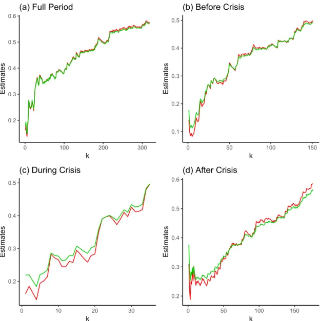
in the linear combination defining the expectHill estimate. To examine the influence of the crisis period on this contribution, we first divide the full period into three subperiods: Before Crisis, from June 15th, 2004, to August 29th, 2008 (1,053 trading days); During Crisis, from September 2nd, 2008, to May 29th, 2009 (185 trading days), and After Crisis, from June 1st, 2009, to June 13th, 2014 (1,259 trading days). For each subperiod, the model assumption of tail heaviness with γ ă 12 is confirmed by the resulting expectHill estimates γ1´k{npαq in Figure 1(b)-(d) and Table 1 in Section A of the Supplementary Material document, for the particular values α “ 0, 12, 1. The estimated optimal values α1´k{n of the weight α
are displayed below in Table 1 (fifth column) for the three subperiods. The corresponding expectHill estimators γ1´k{n are graphed below in Figure 5(b)-(d) against k, along with the Hill estimator pγ1´k{n.
The final pointwise estimates pγ1´k{n and γ1´k{n are shown in Table 1 (third and fourth
columns) for all considered periods. These values are chosen according to the same automatic selection procedure described in Section A of the Supplementary Material document: This selection consists first in computing the standard deviations of the estimator over a moving window large enough to cover around 5% (20% for the crisis period whose length is only 185 trading days) of the possible values of k in the selected range 1 ď k ď n{ log n. The first window over which the standard deviation has a local minimum, and is less than the average standard deviation across all windows, is then selected as the first stable region of the plot. Finally, the value of k which corresponds to the median estimate within this window defines the desired sample fraction.
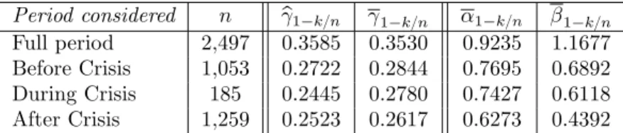
Interestingly, the difference between the obtained Hill and expectHill estimates becomes more pronounced during the crisis period. Also, the linear combination coefficient α1´k{n
decreases during and after the period of crisis, which indicates that the contribution of the asymmetric least squares (expectile-based) component to the estimation procedure increases appreciably with the crisis. We arrive at this same tentative conclusion regarding the evo-lution of the estimated values β1´k{n in (20) of the second combination parameter β, which are displayed in the sixth column of Table 1.
Using the resulting weights α “ α1´k{nand β “ β1´k{nin (24) and (25), we can apply our
two-step method to obtain the QESpn estimates ĆXES‹
p τ1 nppnq :“ ĆXES ‹ p τ1 nppnqpαq and XES ‹ p τ1 nppnq:“ XES‹ p τ1
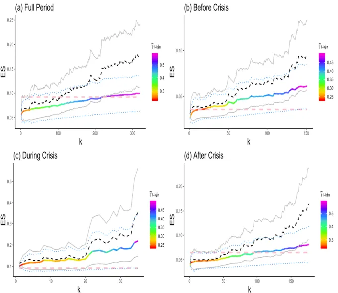
nppnqpα, βq, studied in Theorem6. The plots of these estimates against k are depicted on
Figure 6, for all considered periods, as rainbow curve and dashed black curve, respectively. The effect of the expectHill estimate γ1´k{n on ĆXES‹
p τ1
nppnq is highlighted by a colour-scheme,
ranging from dark red (low γ1´k{n) to dark violet (high γ1´k{n). By Theorem 6, under the bias condition λ1 “ λ2 “ 0, we have
? k logrk{np1 ´ pnqs ˜ Ć XES‹ p τ1 nppnqpαq QESpn ´ 1 ¸ d ÝÑ N p0, vαpγqq,
where vαpγq :“ vα is described in (10). The (symmetric) expectile-based asymptotic
confi-dence interval with conficonfi-dence level 100ϑ% then has the form ĂCIϑpkq “ ĆXES ‹
p τ1
nppnqpαq ˆ I,
where I stands for the interval
I :“ „ 1 ˘ zp1`ϑq{2 log ˆ k np1 ´ pnq ˙ b vα`γ1´k{npαq ˘ {k ,
0.2 0.3 0.4 0.5 0.6 0 100 200 300 k Est ima te s
(a) Full Period
0.1 0.2 0.3 0.4 0.5 0 50 100 150 k Est ima te s (b) Before Crisis 0.2 0.3 0.4 0.5 0 10 20 30 k Est ima te s (c) During Crisis 0.2 0.3 0.4 0.5 0.6 0 50 100 150 k Est ima te s (d) After Crisis
Figure 5: Plots of the Hill and expectHill estimates pγ1´k{n and γ1´k{n against various values
of k, based on daily loss returns of the SPDR S&P 500 ETF (SPY). The estimates depicted on (a)-(d) correspond, respectively, to the full 10-years period (2004-2014) and the three sub-periods: Before Crisis (2004-2008), During Crisis (2008-2009) and After Crisis (2009-2014).
the confidence interval derived from the asymptotic normality of XES‹
p τ1
nppnqpαq, in Theorem6,
can be expressed as CIϑpkq “ XES ‹
p τ1
nppnqpα, βq ˆ I.
The plots of the asymptotic 95% confidence intervals ĂCI0.95pkq and CI0.95pkq against k are
superimposed in Figure 6, respectively, in dotted blue lines and solid grey lines. It can be seen that the (rainbow) paths of the estimates ĆXES‹
p τ1
nppnq and their associated (dotted blue)
confidence bands are less volatile and less pessimistic than, respectively, their corresponding (dashed black) paths of the estimates XES‹
p τ1
nppnq and their associated (solid grey) confidence
bands. In this situation of real-valued profit-loss distributions, we have already provided some Monte Carlo evidence that the estimates ĆXES‹
p τ1
nppnq are more efficient and accurate
relative to their competitors XES‹
p τ1
nppnq.
The final selected pointwise levels ĆXES‹
p τ1 nppnq and XES ‹ p τ1
nppnq, based on minimizing the
standard deviations of the estimates over a moving window, are displayed in the second and fourth columns of Table2, along with their corresponding confidence intervals ĂCI0.95pkq and
CI0.95pkq in the third and fifth columns. The last column indicates the sample maximum loss
Yn,nfor each period. The messages yielded by the two competing methods are broadly similar,
indicating particularly that the expected shortfall (ES) levels differ appreciably before, during and after the crisis period. Clearly, the crisis period exhibits ES levels (around ´11.7% to ´12.7%) three times higher than the pre-crisis period (around ´3.6% to ´3.8%) and about twice and a half higher than the post-crisis period (around ´4.8% to ´4.9%). Also, the ES levels during the crisis period are more conservative than the most catastrophic recorded loss (around ´9.2%), extrapolating thus outside the sample maximum Yn,n.
The theory for our composite expectHill-based estimators ĆXES‹
p τ1 nppnq and XES ‹ p τ1 nppnq is
0.05 0.10 0.15 0.20 0.25 0 100 200 300
k
ES 0.3 0.4 0.5 γ1−k n(a) Full Period
0.05 0.10 0 50 100 150
k
ES 0.25 0.30 0.35 0.40 0.45 γ1−k n(b) Before Crisis
0.1 0.2 0.3 0.4 0.5 0 10 20 30k
ES 0.25 0.30 0.35 0.40 0.45 γ1−k n(c) During Crisis
0.05 0.10 0.15 0.20 0 50 100 150k
ES 0.3 0.4 0.5 γ1−k n(d) After Crisis
Figure 6: Plots of the ES estimates based on daily loss returns of the SPDR S&P 500 ETF (SPY). The estimates ĆXES‹
p τ1
nppnq as rainbow curve and XES
‹
p τ1
nppnqas dashed black curve, along
with the asymptotic 95% confidence intervals ĂCI0.95pkq in dotted blue lines and CI0.95pkq in
0.05 0.10 0.15 0.20 0 20 40 60 80
k
ES
0.25 0.30 0.35 0.40 0.45 0.50 γ1−k n(a) Full Period
0.05 0.10 0 10 20 30 40
k
ES
0.25 0.30 0.35 0.40 0.45 γ1−k n(b) Before Crisis
0.05 0.10 0.15 0.20 0 10 20 30 40k
ES
0.25 0.30 0.35 0.40 0.45 0.50 0.55 γ1−k n(c) After Crisis
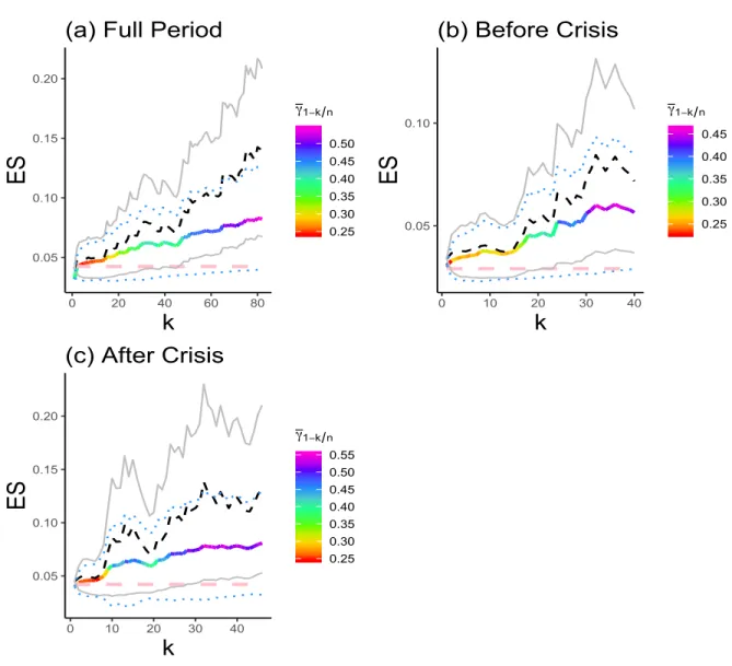
Figure 7: Plots of the ES estimates based on weekly loss returns of the SPDR S&P 500 ETF (SPY). The estimates ĆXES‹
p τ1
nppnq as rainbow curve and XES
‹
p τ1
nppnqas dashed black curve, along
with the asymptotic 95% confidence intervals ĂCI0.95pkq in dotted blue lines and CI0.95pkq in
application to financial returns, the potential serial dependence may then affect the resulting asymptotic confidence intervals. A practical solution to reduce substantially the potential serial dependence in this particular dataset is by using weekly loss returns (corresponding to Wednesdays) in the same sample period. Given the length of the crisis period (38 trading weeks), we perform our extreme value estimation here only for the full period (n “ 516), the pre-crisis period (n “ 219) and the post-crisis period (n “ 259). For each considered period, the final estimates of the tail index γ and the weights α and β are reported in Table3. The plots of the ES estimates ĆXES‹
p τ1 nppnq and XES ‹ p τ1
nppnq against k are graphed in Figure 7, and
the final ES levels along with their corresponding confidence bands are displayed in Table4. By comparing the obtained estimates before the crisis period (third rows in Tables2and 4), it may be seen that the results are quantitatively robust to the change from daily to weekly data. However, both the full period and the post-crisis period suggest fatter tails when moving to weekly data, as indicated by the new expectHill estimates in Table 3.
9
Final comments and perspectives for future research
Let us point out the main conceptual results of this paper that provide a novel take on extreme value analysis using asymmetric least squares estimation. Under the model as-sumption (2) of heavy-tailed distributions with tail index γ ă 1{2, what first distinguishes our contribution is that it introduces a pure expectile-based estimatorrγτn of γ in (6), where
τnis the tuning parameter to be selected in practice. This new estimator has the same form
as the traditional quantile-based Hill estimator pγτn in (7), with the tail empirical quantile
estima-Period considered n γp1´k{n γ1´k{n α1´k{n β1´k{n Full period 2,497 0.3585 0.3530 0.9235 1.1677 Before Crisis 1,053 0.2722 0.2844 0.7695 0.6892 During Crisis 185 0.2445 0.2780 0.7427 0.6118 After Crisis 1,259 0.2523 0.2617 0.6273 0.4392
Table 1: Final estimates of the tail index γ and the combination parameters α and β, based on daily loss returns of the SPDR S&P 500 ETF (SPY) over the full 10-years period (2004-2014) and three sub-periods: Before Crisis (2004-2008), During Crisis (2008-2009) and After Crisis (2009-2014). Period XESĆ ‹ p τ1 nppnq ĂCI0.95 XES ‹ p τ1 nppnq CI0.95 Yn,n Full period 0.0652 (0.0446, 0.0874) 0.0690 (0.0448, 0.0922) 0.0919 Before Crisis 0.0359 (0.0259, 0.0464) 0.0383 (0.0271, 0.0505) 0.0358 During Crisis 0.1169 (0.0784, 0.1597) 0.1277 (0.0842, 0.1712) 0.0919 After Crisis 0.0485 (0.0334, 0.0664) 0.0496 (0.0333, 0.0665) 0.0647
Table 2: Final ES levels with the 95% confidence intervals and the sample maxima. Results based on daily loss returns, with pn “ 1 ´ 1n.
Period considered n pγ1´k{n γ1´k{n α1´k{n β1´k{n Full period 516 0.39094 0.39091 0.9770 1.0625 Before Crisis 219 0.2182 0.2547 0.6506 0.3936 After Crisis 259 0.4316 0.4313 0.9940 1.0158
Table 3: Final estimates of γ, α and β, based on weekly loss returns over the full period (2004-2014) and the two sub-periods: Before (2004-2008) and After (2009-2014) Crisis.
Period ĆXES ‹ p τ1 nppnq ĂCI0.95 XES ‹ p τ1 nppnq CI0.95 Yn,n Full period 0.0609 (0.0305, 0.0872) 0.0748 (0.0328, 0.0925) 0.0424 Before Crisis 0.0364 (0.0232, 0.0490) 0.0378 (0.0248, 0.0507) 0.0292 After Crisis 0.0651 (0.0238, 0.1076) 0.0810 (0.0330, 0.1278) 0.0420
Table 4: Final ES levels with the 95% confidence intervals and the sample maxima. Results based on weekly loss returns, with pn“ 1 ´ n1.