A new methodology for concrete resistivity assessment using the instantaneous polarization response of its metal reinforcement framework

HAL Id: hal-01990082

https://hal.archives-ouvertes.fr/hal-01990082

Submitted on 12 Jun 2019

HAL is a multi-disciplinary open access

archive for the deposit and dissemination of sci-entific research documents, whether they are pub-lished or not. The documents may come from teaching and research institutions in France or abroad, or from public or private research centers.

L’archive ouverte pluridisciplinaire HAL, est destinée au dépôt et à la diffusion de documents scientifiques de niveau recherche, publiés ou non, émanant des établissements d’enseignement et de recherche français ou étrangers, des laboratoires publics ou privés.

A new methodology for concrete resistivity assessment

using the instantaneous polarization response of its

metal reinforcement framework

Gabriel Samson, Fabrice Deby, Jean-Luc Garciaz, Jean Louis Perrin

To cite this version:

Gabriel Samson, Fabrice Deby, Jean-Luc Garciaz, Jean Louis Perrin. A new methodology for concrete resistivity assessment using the instantaneous polarization response of its metal rein-forcement framework. Construction and Building Materials, Elsevier, 2018, 187, pp.531-544. �10.1016/j.conbuildmat.2018.07.158�. �hal-01990082�

1

A new methodology for concrete resistivity assessment using the

instantaneous polarization response of its metal reinforcement

framework

Gabriel Samson1,*, Fabrice Deby1, Jean-Luc Garciaz2, Jean-Louis Perrin2

1 _{LMDC, INSAT/UPS Génie Civil, 135 Avenue de Rangueil, 31077 Toulouse cedex 04}

France.

2 _{LERM SETEC, 23 Rue de la Madeleine, 13631 Arles cedex France}

Abstract

A new methodology is developed to assess concrete cover resistivity using the instantaneous response of the polarization of a metal rebar (galvanostatic pulse method). The instantaneous ohmic drop is linked only with the concrete resistance, which depends on the concrete cover and resistivity, and rebar diameter. A numerical model was developed in Comsol Multiphysics® in order to create a graph linking concrete resistivity to concrete resistance for concrete cover ranging between 1 to 160 mm. This graph and the measured ohmic drop can be used to determine concrete resistivity for any rebar diameter/concrete cover configuration. The theory developed numerically was then confirmed using an experimental setup with controlled water resistivity. The theory is then generalized for counter electrode (CE) diameter ranging from 20 to 70 mm. Finally, the study reveals that the graph developed for a single rebar can be used for any rebar framework density.

Keywords

Resistivity, reinforced concrete structures, corrosion, geometrical factor, one-electrode method, rebar spacing

2

Highlights

 A new concrete resistivity assessment methodology is proposed.

 Resistivity is calculated with a reverse calculation based on 3D numerical model.

 The geometrical factor depends on CE diameter, concrete cover and rebar diameter.

 The numerically developed method was experimentally validated in water.

 The geometrical factor does not depend on rebar framework density.

Graphical abstract

Corresponding author *

Gabriel Samson: samson@insa-toulouse.fr

Acknowledgements

DIAMOND is a collaborative R&D project supported by the French government FUI program, Direction Générale des Entreprises, BPI France and PACA regional council, and accredited by four competitiveness clusters : SAFE, Mer Méditerranée, Nuclear Valley, Alpha RLH.

3

1 Introduction

The corrosion of steel bars is a major issue in the durability of reinforced concrete structures [1]. Corrosion initiation and propagation depend on the concrete durability parameters (porosity, diffusivity, absorption, permeability). However, assessing these parameters on-site is time consuming, expensive and/or requires destructive tests. Resistivity is being increasingly considered as a reliable durability index for assessing the long-term performance of concrete structures [2-4].

Electrical resistivity is defined as the resistance against the flow of an electrical current. It is a specific, geometry-independent property of a material. For concrete, it may vary from 10 to 105 Ω.m [5]. The electrical current is carried by the dissolved ions in the pore solution [6] so resistivity depends on the pore structure, the degree of saturation and the distribution of the ion concentrations in the pore fluid. Concrete resistivity depends on both the concrete production process (water/cement ratio, cement type, mineral admixtures, degree of hydration, curing) and the properties of the concrete in situ (temperature, degree of saturation, ion concentrations in the pore solution) [7]. The latter parameters depend on the production process and the history of external environmental conditions (temperature, relative humidity, air chloride content).

The work presented here is part of the DIAMOND project [8], which aims to create an electrochemical device to assess the corrosion state of reinforced concrete structures by measuring the half-cell corrosion potential Ecorr, the concrete resistivity ρ, and the corrosion

rate icorr, with the same device. This article focusses on measuring concrete resistivity. The

measurement will be performed with a galvanostatic pulse measurement. This technique is employed since around 30 years to determine the corrosion rate of the rebar/concrete interface and the measurement procedure can be found in many papers [9–15]. However, in all these papers, the galvanostatic pulse technique is used to determine the corrosion rate. In these

4 studies, the instantaneous ohmic drop measured, linked with the global concrete electric resistance, is subtracted to the potential response in steady-state regime (in a one dimension way - Randles model) to determine the polarization resistance of the concrete rebar interface (and thus calculate the corrosion rate). We propose here to use this instantaneous ohmic drop to determine the concrete cover resistivity more than the only global resistance. The principle of this resistivity measurement technique is based on the approach initiated by Newman [16] and Feliu et al. [17].

The aim here is to overcome the limitations described in Feliu’s article and to propose a method that could be used for any rebar diameter/concrete cover configuration that may be found on-site and for a wide range of counter-electrode diameter (from 20 to 70 mm).

Our approach is based on a 3D numerical model. The numerically obtained results are used to do a reverse calculation of the resistivity with the instantaneous concrete ohmic resistance measured with the galvanostatic pulse method.

The various existing resistivity measurement techniques are presented first, followed by the newly developed method. The experimental device (DIAMOND probe and experimental validation setup) are introduced. The measurement is modelled numerically using COMSOL software in order to obtain the geometrical factor k, linking the concrete resistance RΩ to the

concrete resistivity ρ for all steel bar diameter/concrete cover configurations. The geometrical factor is also calculated for different counter-electrode (CE) diameter and presented in appendix. The theory developed is then confirmed using the experimental setup. Finally, we demonstrated that the model developed on a single rebar can be applied without modifications for a more or less dense rebar framework which is more representative of what is found on-site.

5

2 Theoretical background: resistivity measurement

There are several resistivity measurement techniques that can be employed. For all of them, the relationship between the resistivity ρ [Ω.m] and the measured resistance RΩ is given in Eq.

1.

𝜌 = 𝑘𝑅_Ω Eq. 1

where RΩ [Ω] is the concrete resistance (e.g. ratio between applied current and measured

potential drop) and k [m] is a geometrical factor that depends on the technique employed and the sample geometry [18]. The two-electrode (or direct) method uses a regular geometry with two electrodes placed face to face (Figure 1 (a)). An alternating current is applied and the potential drop between the electrodes is measured. Usually, a low frequency is employed (from 100 to 1000 Hz). The resistivity ρ [Ω.m], is then calculated with:

𝜌 =𝑆

𝑙𝑅Ω Eq. 2

where S [m2] is the cross-sectional area perpendicular to the current and l [m] is the height of the prismatic or cylindrical concrete sample. However, on-site, this technique cannot be implemented without destructive coring.

On-site, the method most commonly used for resistivity measurement is the Wenner method (four-point method) [19]. Four electrodes are equally spaced (electrode spacing a [m]) on the concrete surface (Figure 1 (b)). The two outer electrodes apply a alternating current and the difference in potential is measured by the inner electrodes. The measured resistance RΩ must

be converted into resistivity using the following equation:

𝜌 = 2𝜋𝑎𝑅_Ω Eq. 3

The resistivity obtained is usually called the apparent resistivity. Eq. 3 is applied for homogeneous semi-infinite volumes. However, experiments have indicated that sample size and the presence of steel bar(s) can lead to erroneous results [4,20–22] and these aspects have to be considered carefully to obtain the correct resistivity value [7]. Both two-electrode and

6 Wenner methods use alternating current in order to prevent the polarization of the metal electrodes.

The one-electrode (or disc-bar) method proposed by Feliu et al. [17] can be employed to measure concrete cover resistivity between a concrete surface and the rebar/concrete interface (Figure 1 (c)). This method is based on the work of Newman [16], who estimated the ohmic drop due to the resistance RΩ between a small disc (the CE) of diameter DCE placed on the

surface of an electrolyte and a large working electrode (WE), placed at infinity (a metal bar). Contrary to the two previous methods, continuous current is employed, in order to polarize the rebar, in steady-state. Theoretically, the electrical resistivity measured between the bar and the CE is:

𝜌 = 2𝐷_𝐶𝐸𝑅_Ω Eq. 4

This relation is theoretically verified only if the metal surface bar area is much greater than the disc area [16]. According to Feliu, in practice, this method can be applied to measure concrete resistivity if the cover thickness is greater than about twice the diameter of the disc being use as the CE [17]. Thus, this method cannot be employed for concrete cover smaller than two CE diameter. The fact that an electrical connection to the steel bar is required explains why this method is hardly ever used for resistivity measurements on-site. However, corrosion rate assessment also requires a connection between the CE and the steel bar [9– 15,23,24]. Using the same device to simultaneously measure concrete resistivity and corrosion rate could help in the evaluation of the corrosion state of a reinforced concrete structure.

7

Figure 1. Principles of resistivity measurements. Two-electrode method (a); Wenner probe (b); one-electrode method (c).

3 General measurement principle

For the one-electrode method, an electrical connection is made to the rebar. The rebar diameter D [m] and concrete cover thickness c [m] can be accurately evaluated by using a non-destructive system such as a pachometer or ground penetrating radar [25].

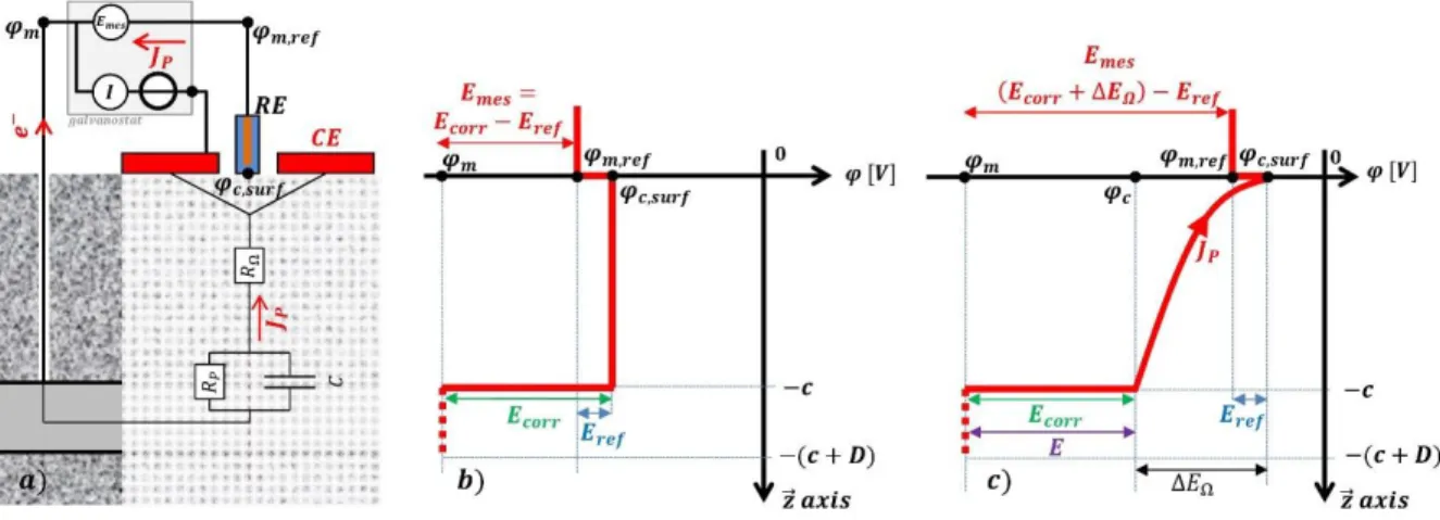
An equivalent electrical circuit is presented in Figure 2 (a). The rebar/concrete interface can be modelled by a Randles equivalent circuit [9], which associates the polarization resistance

RP and the capacitance C. Concrete resistance is RΩ. The polarization of the rebar is a

transient phenomenon. This one-dimensional representation is only qualitative because, in reality, the three-dimensional nature of the problem should be taken into account.

A reference electrode (RE) is used to measure the potential on the surface. The reference potential Eref of the RE is the difference between the absolute potential φm,ref of the metal used

in the probe and its surrounding solution φsol,ref. The reference potential Eref remains constant;

this is why this type of potential measurement electrode is called “reference”. In practice, an electrically conductive material (conductive gel) is placed between the concrete surface and the probe to ensure a good electrical contact (constant potential) between the concrete surface and the surrounding solution inside the probe. The absolute potential in the solution

8 surrounding the RE φsol,ref is then equal to the absolute potential of the concrete at the surface

φc,surf. The corrosion potential Ecorr (half-cell rebar/concrete) is the difference between the

metal rebar absolute potential φm and the surrounding concrete absolute potential φc.

The evolution of absolute potential in the system without polarization (JP = 0) is presented on

the schematic layout of Figure 2 (b). Without polarization, there is no current flowing through the concrete. The absolute potential in the concrete remains constant (φc,surf = φc). The

measured potential Emes is then equal to Ecorr - Eref. The corrosion risk can thus be established

according to the corrosion potential value obtained [1].

Figure 2. Equivalent electrical circuit (a), absolute potential evolution without polarization (b), with polarization, t = 0 (c).

With current injection, in the steady-state, the relation between half-cell potential E and the current density at the rebar/concrete interface is governed by the Butler-Volmer equation [26]. However, the resistivity measurement technique proposed in this article is based on the instantaneous response of the system. The absolute potential evolution at the beginning of the polarization is presented in Figure 2 (c). At this moment, the capacitance acts as a short-cut. The half-cell potential E remains equal to the corrosion potential Ecorr. Thus, the measured

instantaneous ohmic drop ΔEΩ depends only on the injected current JP and concrete resistance

9

Δ𝐸_𝛺 = 𝑅_Ω𝐽_𝑃 Eq. 5

The fact that the rebar is active or passive (or locally active) does not change the instantaneous ohmic drop. It means that this method is particularly interesting when the rebar is locally active and the measurement of the polarization resistance cannot be performed [27,28].

4 Materials and experimental setup

4.1 DIAMOND probe

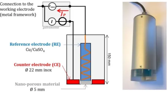
The schematic layout of the DIAMOND probe is presented in Figure 3. The potential at the concrete surface is measured on the centre of the probe, on a small circular surface (5 mm diameter) with a Cu/CuSO4 RE. The CE has a ring shape with 8 mm internal diameter

and 22 mm external diameter (Figure 3). This device is simpler (no guard ring) compared to the commercials devices (i.e. GECOR and GalvaPulse) usually employed to determine rebar corrosion rate. Guard rings are usually associated with confinement problems [12,29,30]. The continuous injected current JP is controlled by a galvanostat developed in our laboratory. It

was calibrated with an Iso-tech multimeter. A photo of the probe is also presented in Figure 3.

10

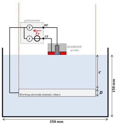
4.2 Geometry of experimental validation setup

We developed a simple setup to validate our model on water (Figure 4). A container (350 mm long, 250 mm wide) was filled with tap and distilled water in various proportions in order to obtain of wide range of water resistivity (from 14 to 1000 Ω.m). Tap water resistivity was 14 Ω.m. The resistivity of the water mixture (true resistivity) was controlled with an Inolab Comb Level 2 conductivity meter. The height of the solution in the container was constant (150 mm). A 300 mm long metal bar (diameter 8, 16, 32 or 50 mm) supported by two small strings was placed horizontally at the centre of the container at various distances (from 5 to 50 mm) from the water surface in order to model different cover thicknesses (Figure 4). The DIAMOND probe was placed at the centre of the water surface, above the centre of the rebar and electrically connected to the bar. Constant current was injected (JP = 10 µA) and the

instantaneous ohmic drop was measured for each rebar diameter/rebar distance from the surface configuration.

11

5 Numerical model

5.1 Constitutive law

The numerical model was set up with a finite element method on COMSOL software with an AC/DC module. Concrete (or water for experimental validation) was assumed to be homogeneous and isotropic (uniform resistivity ρ). In the concrete volume, the electric field is governed by the local Ohm’s law, which links the electrical current density vector j [A/m2] to the electrical field vector E [V/m]:

𝑗 = 1 𝜌𝐸

Eq. 6 In the system, the amount of charge was conserved, which meant that the amount of current flux entering an enclosed surface of a material was equal to the amount of current leaving it:

𝛻. 𝑗 = 0 Eq. 7

5.2 Geometry and mesh

Preliminary numerical work was performed to determine a minimum representative volume for the instantaneous response and steady-state response. It aimed to find the minimum domain size that would not induce size effects in any of the modelled configurations, in order to optimize computation efficiency. The volume found to be most appropriate was 500 x 500 x 300 mm3. The steady-state response depended significantly on the slab geometry but the instantaneous response was hardly influenced by the slab dimensions. Only a quarter of the system was modelled because of the double symmetry of the problem. The DIAMOND probe was placed just over the rebar. The current was injected through the CE. Different CE diameters were modelled (20, 22, 30, 40, 50, 60 and 70 mm). The RE was a cylinder in contact with the surface and the CE was a disc with a hole in it to enable RE contact with surface (Figure 5). The injected current JP was kept at 10 µA for all numerical experiments.

12 RE and CE resistivity was 10-5 _{Ω.m. Different rebar diameters were modelled (4, 8, 16, 32}

and 50 mm). Concrete cover ranged between 1 and 160 mm.

Figure 5. Modelled DIAMOND probe.

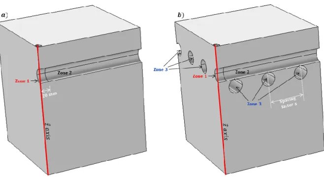
For a single bar, two different zones were defined on the rebar. The first one (zone 1 in Figure 6 (a)) was a 40 mm long zone directly under the probe. The second one (zone 2 in Figure 6 (a)) corresponded to the remaining part of the rebar.

Figure 6. Modelled geometry. D = 32 mm and c = 50 mm. Single bar (a), multiple bar with spacing s = 80 mm (b).

13 On-site, reinforcements are made with a metal framework composed of single perpendicular bars that were regularly spaced and generally electrically connected. To better represent what can be encountered on-site and to investigate the influence of rebar spacing on the concrete resistivity measurement protocol developed, several perpendicular rebars were modelled (Figure 6 (b)). The rebar spacing s was the distance between the central axis of two consecutive parallel bars and it ranged from 40 mm to 280 mm. The probe is placed over the centre of a rebar, at equal distance of the two next perpendicular rebars of the framework (Figure 6 (b)). For this configuration, a third zone was introduced (zone 3 in Figure 6 (b)), corresponding to all the rebar(s)/concrete interface that did not belong to the primary bar (zones 1 and 2).

Tetrahedral elements were used for discretization. The maximum element size was fixed at 0.5 mm. The mesh was refined around the probe, the rebar surface and the 𝑧⃗⃗ axis. The 𝑧⃗⃗ axis was the axis passing through the centre of the RE and the top part of the rebar. It is represented by a red line in Figure 6.

In the simulation, a constant current density was applied to the CE (JP / surface area of the

CE). The corrosion potential of the rebar was imposed Ecorr = - 0.42 V and was intended to

model an active rebar [23,31]. However, changing this potential did not change any of the numerical results given below. A very small electric resistance (0.00001 Ω) was implemented on the rebar/concrete interface to model the polarization resistance short-cut at the beginning of the polarization. All other boundaries were electrically isolated.

6 Results and discussion

6.1 Influence of cover thickness and rebar diameter

Most of the results in the discussion section are presented for a 22 mm CE diameter (DIAMOND probe). The electrical potential on the surface of the domain studied is

14 introduced in Figure 7 for an example where c = 60 mm, D = 32 mm, and ρ = 1000 Ω.m. The potential is maximum on the CE where the current is injected, while it remains equal the corrosion potential at the rebar due the small electrical resistance. Elsewhere in the modelled domain, the potential remains quite constant and small.

Figure 7. Electrical potential on the surface of the studied domain for a concrete cover c of 60 mm, a rebar having a diameter D of 32 mm, and a concrete resistivity ρ of 1000 Ω.m.

To quantitatively visualize the ohmic drop between the surface and the rebar, the electrical potential evolution along the 𝑧 axis is presented in Figure 8. The potential evolution is represented for two concrete covers (10 and 60 mm) and two rebar diameters, 8 mm (straight lines) and 32 mm (dotted lines).

In Figure 8 (a), CE diameter is 22 mm (DIAMOND probe). Without injected current, the potential measured on the surface is equal to the corrosion potential (Ecorr = - 0.42 V). Current

injection leads to a potential ohmic drop between the rebar and the surface. At the beginning of the polarization, on the rebar interface, the potential remains equal to the corrosion potential (see Figure 2 (c)). Thus, the potential measured at the surface minus the corrosion

15 potential represents the instantaneous ohmic drop ΔEΩ between the surface and the rebar.

Figure 8 (a) shows that this ohmic drop depends on concrete cover. The ohmic drop increases with concrete cover. Moreover, the rebar diameter also impacts the ohmic drop, especially if the concrete cover is thin (c = 10 mm, for example, in Figure 8). If the rebar diameter is large, the area through which current can flow is larger and the measured ohmic drop decreases. In Figure 8 (b), the CE diameter is 60 mm. A different potential evolution is observed along the 𝑧 axis. When the CE diameter is increased, the instantaneous ohmic drop decreased for the same reason explaining why the ohmic drop decreased when the rebar diameter is increased.

Figure 8. Electrical potential along 𝒛⃗ axis for two concrete covers (10 and 60 mm) and

two rebar diameters (8 and 32 mm); ρ = 1000 Ω.m; DCE = 22 mm (a), DCE = 60 mm (b).

To visualize concrete cover resistivity influence on potential evolution along the 𝑧 axis, Figure 9 is introduced. Compared to Figure 8, the concrete cover resistivity was divided by ten (i.e. 100 Ω.m). -0,10 -0,08 -0,06 -0,04 -0,02 0,00 -0,42 -0,37 -0,32 -0,27 -0,22 D = 8 mm - c = 10 mm D = 8 mm - c = 60 mm D = 32 mm - c = 10 mm D = 32 mm - c = 60 mm Potential [V] D epth z [m ] single bar DCE= 22 mm ρ = 1000 Ω.m surface -0,10 -0,08 -0,06 -0,04 -0,02 0,00 -0,42 -0,4 -0,38 -0,36 -0,34 D = 8 mm - c = 10 mm D = 8 mm - c = 60 mm D = 32 mm - c = 10 mm D = 32 mm - c = 60 mm Potential [V] D epth z [m ] single bar DCE= 60 mm ρ = 1000 Ω.m surface

16

Figure 9. Electrical potential along 𝒛⃗ axis for two concrete covers (10 and 60 mm) and

two rebar diameters (8 and 32 mm); ρ = 100 Ω.m; DCE = 22 mm.

Reducing concrete cover resistivity significantly reduced the ohmic drop. Similar potential evolutions were observed if the resistivity was changed.

6.2 Geometrical factor k abacus construction

Concrete resistance RΩ does not depend on the injected current. However, concrete resistance

depends on concrete resistivity as shown in Figure 10 for a 10 mm concrete cover. A proportional relationship appears between resistance and resistivity. It can be seen that this relation depends on CE diameter but also on rebar diameter. This relation is also modified with the concrete cover: concrete resistance increases with concrete cover.

-0,10 -0,08 -0,06 -0,04 -0,02 0,00 -0,42 -0,415 -0,41 -0,405 -0,4 D = 8 mm - c = 10 mm D = 8 mm - c = 60 mm D = 32 mm - c = 10 mm D = 32 mm - c = 60 mm Potential [V] D epth z [m ] single bar DCE= 22 mm ρ = 100 Ω.m surface

17

Figure 10. Concrete resistance RΩ [Ω] versus resistivity for two rebar diameters, 8 mm

(dotted lines) and 32 mm (continuous lines) and two CE diameters, 22 mm (full markers) and 60 mm (empty markers).

The slope k, (ratio between concrete resistance and concrete resistivity) was calculated for several configurations that can be encountered on-site and is presented in Figure 11 for two CE diameters (22 mm (a), 60 mm (b)) for concrete cover ranging from 10 to 160 mm. On-site, most concrete covers exceed 10 mm. However, reinforced concrete structure can suffer from construction defects which lead to very thin concrete cover and associated corrosion problems. It explains why we decided to determine the slope k for concrete cover ranging from 1 to 160 mm so that the reader can use the presented abacus (appendix) for any cover find on-site. The slope k is then referred to as the geometrical factor. For the sake of clarity, only five rebar diameters are presented.

For 22 mm CE diameter (Figure 11 (a)), if the concrete cover is thicker than 10 mm, the geometrical factor k no longer depends almost solely on rebar diameter. The relation between concrete resistance and concrete resistivity mostly depends on the concrete cover. When the concrete cover is very small (< 10 mm, appendix), k increases significantly with rebar

0 2 000 4 000 6 000 8 000 10 000 12 000 14 000 16 000 0 200 400 600 800 1000 D = 8 mm - c = 10 mm D = 32 mm - c = 10 mm Resistivity ρ [Ω] Concrete resistance RΩ[Ω] single bar JP= 10 µA DCE= 22 mm DCE= 60 mm

18 diameter. Moreover, we added the analytical result by Feliu [17] that obtain a geometrical factor equal to 2DCE (44 mm for our device). Feliu specified that this formula can only be

applied when the concrete cover is greater than about twice diameter of the CE. This area corresponds to the grey section in Figure 11. This validity area is also represented in the appendix by values in italics for each CE diameter. The results obtained by our model and obtained by Feliu perfectly match for the higher concrete cover simulated (160 mm). However, differences appeared even when the cover is equal to twice CE diameter. The 3D numerical simulation we developed can now be employed to obtain the geometrical factor when the concrete cover is smaller than this limit (c < 44 mm). Our CE is quite small (DCE = 22 mm) which means that the Feliu’s model can only be applied when the concrete

cover is bigger than 44 mm which is a value that can be found on-site. However, bigger CE can be found on literature (i.e. 70 mm for GECOR and 60 mm for Galvapulse [12]) which mean that the Feliu model could only be applied for very thick concrete covers that are rarely found on-site. The Feliu validity area decreases when the CE diameter is increased as shown on both Figure 11 and appendix by values in italics. For example, with a 60 mm diameter CE (Figure 11 (b)), the k slope value given by Feliu model is 0.12 mm (for all concrete covers and rebar diameters). The numerical simulation shows that for a concrete cover of 30 mm, for a 16 mm rebar diameter the k slope is 0.169 (Figure 11 (b) or appendix) which corresponds to an error of around 30%. With a 10 mm concrete cover the error reach 55 % (k = 0.263). Feliu model leads to concrete resistivity underestimation when the concrete cover is less than two CE diameters, as announced by the authors.

19

Figure 11. Geometrical factor k of a single rebar depending on concrete cover for five rebar diameters and Feliu’s geometrical factor. Values can be find in appendix.

6.3 Resistivity measurement procedure

The experimental procedure for determining concrete resistivity on-site is:

- CE diameter DCE, concrete cover c and rebar diameter D measurements

- k geometrical factor determination (Figure 11 or appendix)

- DIAMOND probe positioning above the centre of the rebar

- Instantaneous ohmic drop ΔEΩ measurement

- Concrete resistance RΩ calculation

- Concrete cover resistivity calculation (ρ = k.RΩ)

This method can be employed for micro or macro-cell corrosion systems since the polarization resistance is short-cut.

6.4 Experimental validation

This resistivity calculation procedure was employed on the water tank filled with water of known resistivity (true resistivity). Water resistance RΩ was experimentally evaluated for 84

0,040 0,045 0,050 0,055 0,060 0,065 0,070 0,075 10 100 k geometrical factor [m] P Concrete cover c [mm] Feliu model validity area kFeliu= 2DCE(0.044 m) limi t: x = 2 DCE 44 DCE= 22 mm 0,10 0,15 0,20 0,25 0,30 10 100 k geometrical factor [m] P Concrete cover c [mm] Fel iu mod el v a lid it y a rea kFeliu= 2DCE(0.120 m) limi t: x = 2 DCE 120 DCE= 60 mm

20 configurations (7 water covers, 6 water resistivities and 4 rebar diameters) with the 22 mm probe. Water resistance increases with water resistivity and cover.

The measured resistances were then multiplied by the numerically determined geometrical factor k (Figure 11 (a)) to calculate the water resistivities (Figure 12):

Figure 12. Resistivity ρ [Ω.m], calculated with k factor (Figure 11 (a)) according to the concrete cover for two rebar diameters, 8 mm (dotted lines) and 32 mm (continuous lines). Straight lines are true resistivities. Hollow lines are Feliu resistivity (D = 8 mm). ρ = 14, 40 and 100 Ω.m (a), ρ = 250, 500 and 1000 Ω.m (b) .

A good correlation was obtained between the calculated and the true resistivities (straight horizontal lines in Figure 12) for all rebar diameter/water cover configurations tested, which validated the numerical approach developed in this article. However, calculated resistivities remained slightly higher than the true resistivities. Calculated values were 5 % higher than real ones on average. An internal resistance in our experimental system that was not taken into account in our numerical model may explain the small differences observed. The resistivity calculated with the Feliu’s analytical formulae is also represented for D = 8 mm

1 10 100 0 10 20 30 40 50 ρ = 100 Ω.m ρ = 40 Ω.m ρ = 14 Ω.m Water cover c [mm] Water resisitivity 𝜌 [Ω.m] 100 1 000 0 10 20 30 40 50 ρ = 1000 Ω.m ρ = 500 Ω.m ρ = 250 Ω.m Water cover c [mm] Water resisitivity 𝜌 [Ω.m]

21 (with hollow lines - Figure 12). As expected, the calculated resistivity are in good correlation with the true resistivity when the concrete cover exceed twice the diameter (i.e. 44 mm).

6.5 Influence of rebar spacing

The influence of the rebar spacing factor s on the concrete resistivity estimation was investigated numerically. With a mesh of rebars (Figure 6 (b)), the relation between concrete resistance and concrete resistivity might be different from what was modelled for a single bar as the proximity of the other rebars could modify the ohmic drop. The spacing factor s, (distance between the central axes of two consecutive parallel bars) may influence the k geometrical factor created (Figure 11 and appendix). A single rebar corresponds to an infinite

s. Four rebar spacings (40, 80, 120 and 240 mm) were investigated. The next results are

obtained for a 22 mm CE diameter.

The investigation began by following current lines through the modelled concrete block on a single rebar diameter/concrete cover configuration (c = 50 mm, D = 32 mm) for three different rebar spacings (∞ (single bar), 240 and 80 mm). The total current received by the three zones defined in Figure 6 (b) is detailed In Table 1. For a single bar, around a quarter of the injected current flowed through zone 1 (25.5 %), the other part flowing through zone 2. Reducing the spacing factor resulted in other bars being taken into account, which enabled the current to disperse and to flow through these new rebar/concrete interfaces (zone 3). Thus, the percentages of current flowing through zones 1 and 2 decreased when the spacing factor decreased.

22

Table 1. Current distribution in the three zones for 50 mm concrete cover and three spacing factors (∞, 240 and 80 mm) for a total of 2000 current lines. D = 32 mm. DCE =

22 mm. Current % zone n° 1 2 3 s [mm] ∞ 25.5 74.5 0.0 240 23.4 48.5 28.1 80 19.9 34.6 45.6

23

Figure 13. Current line distribution for concrete cover of 50 mm and rebar diameter of 32 mm. s = ∞ (a), s = 240 mm (b), s = 80 mm (c). DCE = 22 mm. Red (zone 1 - 4 cm area),

black (zone 2 - the rest of the primary bar), blue (zone 3 - other bar(s)).

Figure 13 gives a visual representation of the current distribution. For each configuration, 2000 current lines are represented. Three colours have been introduced to distinguished current lines flowing through the three zones (zone 1 = red, zone 2 = black, zone 3 = blue). Current line distribution for a single bar (s = ∞) is presented in Figure 13 (a). Current lines are distributed through the concrete block.

When the spacing factor is reduced (s = 240 mm - Figure 13 (b)), part of the current goes from the CE to the new bars (blue streamlines). In this particular example, it corresponds to 28.1 % of the injected current. However, the proportion of current received by zone 1 changes only slightly (from 25.5 to 23.4 %). Adding other bars (s = 80 mm - Figure 13 (c)) reduces the current received by the initial bar, especially by zone 2.

Figure 14 quantifies how the current distribution evolves with concrete cover and rebar spacing. In Figure 14 (a), only a single rebar is considered. With very thin concrete cover, the majority of the current goes through zone 1, especially if the rebar diameter is large. In this configuration (22 mm diameter probe), the current percentage flowing through zone 1 is always higher if the rebar diameter is large. Increasing the concrete cover tends to distribute the current along the bar and the current percentage going through zone 2 increases (dotted lines in Figure 14 (a)).

Adding other bars (Figure 14 (b) and (c)) modifies the current distribution. However, the proportion of current flowing through zone 1 (continuous lines in Figure 14) is hardly modified by the spacing factor. Adding bars mostly modifies the current received by zone 2.

25

Figure 14. Current distribution in the three zones of the rebars according to concrete cover for two rebar diameters, 8 mm (green lines) and 32 mm (black lines). DCE

= 22 mm. s = ∞ (a), s = 240 mm (b), s = 80 mm (c).

Figure 15 precisely quantifies the current distribution for the different spacing factors modelled considering a constant rebar diameter (8 mm). The current flowing through zone 1 is presented in Figure 15 (a). As could be sensed in Figure 14, the proportion of current flowing through zone 1 does not evolve greatly with rebar spacing and is maximum for a single rebar.

In contrast, the proportion of current flowing through zone 2 depends heavily on the rebar spacing (Figure 15 (b)) but, whatever the rebar spacing considered, the current received in zone 2 remains small if the concrete cover is small as the majority of the current goes through zone 1. The proportion of current flowing through zone 2 decreases if rebar spacing decreases because a significant part of the current flows through zone 3. Similar conclusions can be drawn for other rebar diameters.

26

Figure 15. Current distributions according to concrete cover and rebar spacing. Rebar diameter = 32 mm. DCE = 22 mm. Zone 1 (a), zone 2 (b), zone 3 (c).

27 The evolution of the ohmic drop for two rebar diameters (8 and 32 mm) and three rebar spacings (∞, 240 and 80 mm) is presented in Figure 16. This figure makes it clear that the ohmic drop does not depend on rebar spacing and depends only on concrete cover and rebar diameter. The differences observed when the spacing factor is modified are always lower than 2%.This means that the geometrical factor k, presented on Figure 11 can be used for any rebar spacing factor. The only parameters required to determine the concrete resistivity are the concrete cover, the rebar diameter and the measured ohmic drop. Similar conclusions were made for all the tested CE diameters.

Figure 16. Ohmic drop ΔEΩ in concrete according to concrete cover for two rebar

diameters (8 and 32 mm) and three rebar spacings (∞, 240 and 80 mm); ρ = 1000 Ω.m. 7 Conclusions

A new device to assess concrete resistivity has been proposed. Its geometry is simple (no guard ring): the current is injected through an annular CE and the potential is measured on the surface. The resistivity measurement developed is based on the instantaneous ohmic drop measured at the beginning of the polarization. A numerical model was set up in COMSOL Multiphysics® in order to link the measured ohmic drop to the concrete resistivity, knowing rebar diameter and concrete cover. The built abacuses can be used to determine concrete resistivity for a wide range of concrete cover, from 1 to 160 mm (unlike the previous model

28 by Feliu). The model is generalized for a wide range a CE diameter (from 20 to 70 mm) and presented on a summary table in appendix. The theory developed was confirmed by experiments performed on water of known resistivity. This methodology (measurement and 3D reverse calculation) can be used by the researchers or engineers that use galvanostatic measurements to measure the corrosion rate of the metal rebar to also determine the concrete cover resistivity. This method can be used for both micro- and macro-cell corrosion systems. Finally, the influence of the rebar framework on the developed procedure was investigated numerically. The investigations proved that the graphs established are independent of the rebar spacing (unlike in the Wenner method). The methodology was built with homogeneous material and with a perfect electrical contact between the probe and the concrete. Furthers works are required to investigate the ability of the probe to measure the concrete cover on real concrete structure.

29

8 Appendix: geometrical factor k depending on rebar diameter and concrete cover for different CE diameter. Values in italics represent the Feliu validity model area (concrete cover ≥ 2DCE) as depicted in grey in Figure 11.

CE diameter [mm] Concrete cover c [mm] Rebar diameter D [mm] 1 2 3 4 5 7.5 10 12.5 15 20 30 40 50 60 70 80 100 120 140 160 20 4 0.145 0.108 0.090 0.080 0.073 0.063 0.057 0.054 0.051 0.048 0.045 0.044 0.043 0.042 0.042 0.042 0.041 0.041 0.041 0.040 6 0.161 0.116 0.096 0.084 0.076 0.064 0.058 0.054 0.052 0.049 0.046 0.044 0.043 0.043 0.042 0.042 0.042 0.041 0.041 0.041 8 0.174 0.122 0.100 0.087 0.078 0.066 0.059 0.055 0.052 0.049 0.046 0.045 0.044 0.043 0.042 0.042 0.042 0.041 0.041 0.041 10 0.184 0.127 0.103 0.089 0.080 0.067 0.060 0.056 0.053 0.049 0.046 0.044 0.044 0.043 0.043 0.042 0.042 0.041 0.041 0.041 12 0.193 0.132 0.106 0.091 0.082 0.068 0.060 0.056 0.053 0.050 0.046 0.045 0.044 0.043 0.043 0.042 0.042 0.042 0.041 0.041 14 0.201 0.136 0.109 0.093 0.083 0.069 0.061 0.056 0.053 0.050 0.046 0.045 0.044 0.043 0.043 0.042 0.042 0.042 0.041 0.041 16 0.207 0.140 0.111 0.094 0.084 0.069 0.061 0.056 0.053 0.050 0.046 0.045 0.044 0.043 0.043 0.043 0.042 0.042 0.041 0.041 20 0.219 0.145 0.114 0.097 0.085 0.070 0.062 0.057 0.054 0.050 0.047 0.045 0.044 0.043 0.043 0.043 0.042 0.042 0.041 0.041 25 0.231 0.151 0.118 0.099 0.087 0.070 0.062 0.058 0.054 0.050 0.047 0.045 0.044 0.044 0.043 0.043 0.042 0.042 0.042 0.041 32 0.245 0.157 0.121 0.101 0.089 0.072 0.063 0.058 0.055 0.051 0.047 0.045 0.044 0.044 0.043 0.043 0.042 0.042 0.042 0.042 50 0.267 0.166 0.126 0.105 0.091 0.074 0.064 0.059 0.056 0.051 0.047 0.046 0.045 0.044 0.043 0.043 0.042 0.042 0.042 0.042 22 4 0.162 0.121 0.102 0.091 0.083 0.071 0.065 0.061 0.057 0.054 0.050 0.049 0.048 0.047 0.047 0.046 0.046 0.045 0.045 0.045 6 0.181 0.131 0.109 0.095 0.087 0.073 0.066 0.062 0.059 0.055 0.051 0.049 0.048 0.047 0.047 0.047 0.046 0.045 0.045 0.045 8 0.194 0.139 0.114 0.099 0.089 0.075 0.067 0.063 0.059 0.055 0.051 0.050 0.048 0.048 0.047 0.047 0.046 0.046 0.045 0.045 10 0.207 0.145 0.118 0.102 0.091 0.076 0.068 0.063 0.059 0.056 0.052 0.050 0.049 0.048 0.047 0.047 0.046 0.046 0.046 0.045 12 0.217 0.151 0.122 0.105 0.094 0.078 0.069 0.064 0.060 0.056 0.052 0.050 0.049 0.048 0.048 0.047 0.046 0.046 0.046 0.045 14 0.226 0.155 0.124 0.107 0.095 0.078 0.069 0.064 0.060 0.056 0.052 0.050 0.049 0.048 0.048 0.047 0.046 0.046 0.046 0.045 16 0.234 0.159 0.127 0.109 0.097 0.079 0.070 0.064 0.061 0.056 0.052 0.050 0.049 0.048 0.047 0.047 0.046 0.046 0.046 0.045 20 0.248 0.166 0.132 0.112 0.099 0.081 0.070 0.065 0.062 0.056 0.052 0.050 0.049 0.048 0.048 0.047 0.047 0.046 0.046 0.045 25 0.263 0.173 0.135 0.114 0.100 0.082 0.072 0.066 0.062 0.057 0.053 0.050 0.049 0.048 0.048 0.047 0.047 0.046 0.046 0.046 32 0.279 0.180 0.140 0.118 0.103 0.082 0.072 0.066 0.062 0.057 0.053 0.050 0.049 0.049 0.048 0.048 0.047 0.047 0.046 0.046 50 0.308 0.194 0.148 0.122 0.106 0.084 0.074 0.067 0.063 0.058 0.053 0.051 0.050 0.049 0.048 0.048 0.047 0.047 0.046 0.046 30 4 0.231 0.175 0.149 0.133 0.122 0.105 0.095 0.088 0.083 0.077 0.071 0.067 0.066 0.064 0.063 0.063 0.062 0.061 0.060 0.060 6 0.259 0.191 0.160 0.142 0.128 0.109 0.097 0.090 0.085 0.078 0.071 0.068 0.066 0.065 0.064 0.063 0.062 0.061 0.061 0.060 8 0.282 0.204 0.169 0.148 0.134 0.112 0.100 0.092 0.086 0.079 0.072 0.069 0.067 0.065 0.064 0.064 0.063 0.062 0.061 0.061 10 0.301 0.216 0.176 0.154 0.138 0.115 0.102 0.093 0.087 0.080 0.072 0.069 0.067 0.066 0.065 0.064 0.063 0.062 0.061 0.061 12 0.318 0.224 0.183 0.158 0.142 0.116 0.103 0.094 0.088 0.081 0.073 0.069 0.067 0.066 0.065 0.064 0.063 0.062 0.061 0.061 14 0.334 0.232 0.188 0.162 0.145 0.119 0.104 0.095 0.089 0.081 0.073 0.069 0.068 0.066 0.065 0.064 0.063 0.062 0.062 0.061 16 0.346 0.240 0.193 0.166 0.147 0.120 0.105 0.096 0.089 0.081 0.074 0.070 0.068 0.066 0.065 0.064 0.063 0.062 0.062 0.061 20 0.370 0.251 0.201 0.171 0.151 0.123 0.106 0.097 0.090 0.082 0.074 0.070 0.068 0.066 0.065 0.065 0.063 0.063 0.062 0.062 25 0.395 0.265 0.209 0.177 0.155 0.125 0.108 0.098 0.091 0.083 0.074 0.070 0.068 0.067 0.066 0.065 0.064 0.063 0.062 0.062 32 0.423 0.280 0.218 0.184 0.161 0.128 0.110 0.100 0.092 0.083 0.075 0.071 0.069 0.067 0.066 0.065 0.064 0.063 0.062 0.062 50 0.477 0.306 0.235 0.195 0.169 0.133 0.113 0.102 0.094 0.084 0.076 0.072 0.069 0.068 0.067 0.066 0.064 0.064 0.063 0.063 40 4 0.317 0.242 0.208 0.188 0.173 0.149 0.135 0.125 0.118 0.108 0.097 0.092 0.089 0.087 0.085 0.084 0.082 0.081 0.080 0.079 6 0.359 0.267 0.227 0.201 0.185 0.157 0.141 0.129 0.121 0.110 0.099 0.093 0.090 0.088 0.086 0.085 0.083 0.082 0.081 0.080

30 8 0.392 0.288 0.241 0.212 0.193 0.163 0.145 0.132 0.123 0.112 0.100 0.095 0.091 0.088 0.087 0.085 0.084 0.082 0.081 0.080 10 0.421 0.305 0.253 0.221 0.201 0.167 0.148 0.135 0.126 0.114 0.101 0.095 0.092 0.089 0.087 0.086 0.084 0.083 0.081 0.081 12 0.445 0.319 0.263 0.229 0.206 0.171 0.150 0.137 0.127 0.115 0.102 0.095 0.092 0.090 0.088 0.086 0.084 0.083 0.082 0.081 14 0.468 0.332 0.272 0.236 0.211 0.175 0.152 0.139 0.129 0.116 0.103 0.096 0.092 0.090 0.088 0.087 0.085 0.083 0.082 0.081 16 0.488 0.344 0.281 0.242 0.216 0.177 0.155 0.140 0.130 0.117 0.103 0.097 0.093 0.090 0.088 0.087 0.085 0.084 0.083 0.081 20 0.525 0.364 0.294 0.252 0.224 0.182 0.158 0.142 0.132 0.118 0.104 0.097 0.093 0.091 0.089 0.087 0.085 0.084 0.083 0.082 25 0.563 0.386 0.309 0.263 0.233 0.187 0.162 0.145 0.134 0.119 0.105 0.098 0.094 0.091 0.089 0.088 0.086 0.084 0.083 0.082 32 0.610 0.411 0.326 0.276 0.242 0.192 0.164 0.148 0.136 0.121 0.106 0.098 0.094 0.091 0.090 0.088 0.086 0.085 0.084 0.082 50 0.699 0.458 0.356 0.297 0.258 0.201 0.172 0.153 0.139 0.123 0.107 0.100 0.095 0.092 0.091 0.089 0.087 0.085 0.084 0.083 50 4 0.402 0.309 0.268 0.242 0.224 0.195 0.177 0.164 0.154 0.141 0.126 0.118 0.113 0.110 0.107 0.105 0.102 0.100 0.099 0.097 6 0.458 0.344 0.293 0.262 0.241 0.207 0.185 0.170 0.160 0.145 0.128 0.120 0.115 0.111 0.109 0.106 0.104 0.102 0.100 0.099 8 0.503 0.372 0.314 0.279 0.254 0.215 0.192 0.175 0.164 0.148 0.130 0.122 0.116 0.112 0.110 0.108 0.105 0.103 0.101 0.099 10 0.540 0.396 0.331 0.291 0.264 0.222 0.197 0.179 0.167 0.150 0.132 0.123 0.117 0.113 0.110 0.108 0.105 0.103 0.102 0.100 12 0.575 0.416 0.345 0.302 0.274 0.228 0.201 0.183 0.170 0.152 0.133 0.124 0.118 0.114 0.111 0.109 0.106 0.104 0.102 0.101 14 0.605 0.434 0.358 0.313 0.282 0.233 0.205 0.186 0.172 0.154 0.134 0.125 0.118 0.115 0.112 0.110 0.106 0.104 0.103 0.101 16 0.633 0.451 0.370 0.322 0.289 0.238 0.208 0.188 0.174 0.155 0.135 0.125 0.119 0.115 0.112 0.110 0.107 0.105 0.103 0.102 20 0.682 0.480 0.390 0.338 0.301 0.246 0.214 0.193 0.177 0.158 0.137 0.126 0.120 0.116 0.113 0.111 0.107 0.105 0.103 0.102 25 0.736 0.510 0.413 0.355 0.315 0.254 0.219 0.197 0.181 0.160 0.138 0.127 0.121 0.117 0.114 0.112 0.108 0.106 0.104 0.103 32 0.801 0.547 0.438 0.373 0.329 0.263 0.226 0.201 0.184 0.162 0.139 0.128 0.122 0.118 0.114 0.112 0.109 0.107 0.105 0.103 50 0.929 0.618 0.485 0.408 0.356 0.279 0.237 0.209 0.190 0.167 0.142 0.130 0.123 0.119 0.116 0.113 0.110 0.108 0.106 0.104 60 4 0.485 0.376 0.326 0.296 0.275 0.240 0.218 0.203 0.191 0.174 0.155 0.144 0.137 0.133 0.129 0.127 0.123 0.120 0.118 0.116 6 0.556 0.420 0.360 0.323 0.297 0.256 0.230 0.213 0.199 0.180 0.159 0.147 0.140 0.135 0.131 0.129 0.125 0.122 0.119 0.117 8 0.612 0.456 0.386 0.344 0.315 0.268 0.240 0.220 0.205 0.185 0.162 0.150 0.142 0.137 0.133 0.130 0.126 0.123 0.121 0.119 10 0.661 0.487 0.409 0.362 0.329 0.279 0.247 0.226 0.210 0.188 0.164 0.151 0.143 0.138 0.134 0.131 0.127 0.124 0.122 0.119 12 0.704 0.513 0.428 0.377 0.342 0.287 0.253 0.231 0.214 0.191 0.166 0.153 0.145 0.139 0.135 0.132 0.128 0.125 0.122 0.120 14 0.742 0.536 0.445 0.391 0.353 0.294 0.259 0.235 0.218 0.194 0.168 0.154 0.146 0.140 0.136 0.133 0.129 0.125 0.123 0.121 16 0.778 0.559 0.461 0.403 0.363 0.301 0.263 0.239 0.221 0.196 0.169 0.155 0.147 0.141 0.137 0.134 0.129 0.126 0.123 0.121 20 0.841 0.597 0.489 0.424 0.380 0.312 0.272 0.245 0.225 0.199 0.171 0.157 0.148 0.142 0.138 0.135 0.130 0.127 0.124 0.122 25 0.910 0.639 0.518 0.447 0.398 0.323 0.280 0.252 0.230 0.203 0.174 0.158 0.149 0.143 0.139 0.136 0.131 0.128 0.125 0.123 32 0.992 0.687 0.552 0.473 0.419 0.337 0.290 0.258 0.236 0.207 0.176 0.160 0.151 0.144 0.140 0.137 0.132 0.129 0.126 0.124 50 1.161 0.783 0.618 0.523 0.459 0.362 0.307 0.271 0.246 0.213 0.180 0.163 0.153 0.147 0.142 0.139 0.134 0.130 0.128 0.126 70 4 0.568 0.441 0.383 0.349 0.325 0.285 0.260 0.242 0.229 0.209 0.185 0.171 0.162 0.156 0.152 0.148 0.143 0.139 0.136 0.134 6 0.653 0.496 0.425 0.383 0.353 0.306 0.276 0.255 0.240 0.217 0.190 0.176 0.166 0.160 0.155 0.151 0.146 0.142 0.138 0.136 8 0.722 0.541 0.459 0.410 0.376 0.322 0.289 0.266 0.248 0.223 0.195 0.179 0.169 0.162 0.157 0.153 0.148 0.143 0.140 0.137 10 0.781 0.579 0.487 0.432 0.395 0.335 0.299 0.274 0.255 0.228 0.198 0.181 0.171 0.164 0.159 0.155 0.149 0.145 0.141 0.139 12 0.833 0.612 0.512 0.452 0.411 0.346 0.307 0.280 0.260 0.232 0.201 0.183 0.173 0.165 0.160 0.156 0.150 0.146 0.142 0.140 14 0.881 0.640 0.534 0.469 0.425 0.356 0.315 0.286 0.265 0.236 0.203 0.185 0.174 0.167 0.161 0.157 0.151 0.147 0.143 0.141 16 0.923 0.668 0.554 0.485 0.438 0.365 0.321 0.291 0.269 0.239 0.205 0.187 0.175 0.168 0.162 0.158 0.152 0.148 0.144 0.141 20 1.001 0.716 0.589 0.514 0.461 0.380 0.332 0.300 0.276 0.244 0.208 0.189 0.177 0.169 0.164 0.159 0.153 0.149 0.145 0.143 25 1.086 0.767 0.626 0.542 0.485 0.396 0.344 0.308 0.284 0.249 0.211 0.191 0.179 0.171 0.165 0.161 0.155 0.150 0.147 0.144 32 1.186 0.828 0.670 0.576 0.512 0.414 0.357 0.319 0.292 0.255 0.215 0.194 0.181 0.173 0.167 0.162 0.156 0.151 0.148 0.145 50 1.395 0.951 0.756 0.644 0.566 0.448 0.381 0.337 0.306 0.265 0.221 0.198 0.185 0.176 0.170 0.165 0.158 0.154 0.150 0.147

31

9 Acknowledgements

DIAMOND is a collaborative R&D project supported by the French government FUI program, Direction Générale des Entreprises, BPI France and PACA regional council, and accredited by four competitiveness clusters : SAFE, Mer Méditerranée, Nuclear Valley, Alpha RLH.

10 References

[1] W. Morris, A. Vico, M. Vazquez, S.R. de Sanchez, Corrosion of reinforcing steel evaluated by means of concrete resistivity measurements, Corros. Sci. 44 (2002) 81–99. doi:10.1016/S0010-938X(01)00033-6.

[2] W.J. McCarter, H.M. Taha, B. Suryanto, G. Starrs, Two-point concrete resistivity measurements: interfacial phenomena at the electrode–concrete contact zone, Meas. Sci. Technol. 26 (2015) 085007. doi:10.1088/0957-0233/26/8/085007.

[3] M.G. Alexander, Y. Ballim, K. Stanish, A framework for use of durability indexes in performance-based design and specifications for reinforced concrete structures, Mater. Struct. 41 (2008) 921–936. doi:10.1617/s11527-007-9295-0.

[4] K. Reichling, M. Raupach, N. Klitzsch, Determination of the distribution of electrical resistivity in reinforced concrete structures using electrical resistivity tomography: ERT on reinforced concrete, Mater. Corros. 66 (2015) 763–771. doi:10.1002/maco.201407763.

[5] R.B. Polder, Test methods for on site measurement of resistivity of concrete — a RILEM TC-154 technical recommendation, Constr. Build. Mater. 15 (2001) 125–131. doi:10.1016/S0950-0618(00)00061-1.

[6] H. Yildirim, T. Ilica, O. Sengul, Effect of cement type on the resistance of concrete against chloride penetration, Constr. Build. Mater. 25 (2011) 1282–1288. doi:10.1016/j.conbuildmat.2010.09.023.

[7] A.J. Garzon, J. Sanchez, C. Andrade, N. Rebolledo, E. Menéndez, J. Fullea, Modification of four point method to measure the concrete electrical resistivity in presence of reinforcing bars, Cem. Concr. Compos. 53 (2014) 249–257. doi:10.1016/j.cemconcomp.2014.07.013.

[8] DIAMOND project, Proj. Diam. - Diagn. Corros. Béton Armé - Sonde Captae. (2017). https://www.projet-diamond.com (accessed May 11, 2017).

[9] C.J. Newton, J.M. Sykes, A galvanostatic pulse technique for investigation of steel corrosion in concrete, Corros. Sci. 28 (1988) 1051–1074. doi:10.1016/0010-938X(88)90101-1.

[10] B. Elsener, O. Klinghoffer, T. Frolund, E. Rislund, Y. Schiegg, H. Böhni, Assessment of reinforcement corrosion by means of galvanostatic pulse technique, in: Norway, 1997. [11] P.V. Nygaard, Non-destructive elecrochemical monitoring of reinforcement corrosion,

Technical University of Denmark (DTU), 2009.

[12] P.V. Nygaard, M.R. Geiker, B. Elsener, Corrosion rate of steel in concrete: evaluation of confinement techniques for on-site corrosion rate measurements, Mater. Struct. 42 (2009) 1059–1076. doi:10.1617/s11527-008-9443-1.

[13] P.V. Nygaard, M.R. Geiker, Measuring the corrosion rate of steel in concrete – effect of measurement technique, polarisation time and current, Mater. Corros. 63 (2012) 200– 214. doi:10.1002/maco.201005792.

32 [14] C. Andrade, C. Alonso, On-site measurements of corrosion rate of reinforcements,

Constr. Build. Mater. 15 (2001) 141–145. doi:10.1016/S0950-0618(00)00063-5.

[15] C. Andrade, C. Alonso, Test methods for on-site corrosion rate measurement of steel reinforcement in concrete by means of the polarization resistance method, Mater. Struct. 37 (2004) 623–643. doi:10.1007/BF02483292.

[16] J. Newman, Resistance for Flow of Current to a Disk, J. Electrochem. Soc. 113 (1966) 501–502. doi:10.1149/1.2424003.

[17] S. Feliu, C. Andrade, J.A. González, C. Alonso, A new method for in-situ measurement of electrical resistivity of reinforced concrete, Mater. Struct. 29 (1996) 362–365. doi:10.1007/BF02486344.

[18] H. Layssi, P. Ghods, A.R. Alizadeh, M. Salehi, Electrical Resistivity of Concrete, Concr. Int. 37 (2015) 41–46.

[19] F. Wenner, A method of measuring earth resistivity, Govt. Print. Off., 1916.

[20] J. Sanchez, C. Andrade, J. Torres, N. Rebolledo, J. Fullea, Determination of reinforced concrete durability with on-site resistivity measurements, Mater. Struct. 50 (2017) 41. doi:10.1617/s11527-016-0884-7.

[21] F. Presuel-Moreno, Y. Liu, Y.-Y. Wu, Numerical modeling of the effects of rebar presence and/or multilayered concrete resistivity on the apparent resistivity measured via the Wenner method, Constr. Build. Mater. 48 (2013) 16–25. doi:10.1016/j.conbuildmat.2013.06.053.

[22] M. Salehi, P. Ghods, O.B. Isgor, Numerical investigation of the role of embedded reinforcement mesh on electrical resistivity measurements of concrete using the Wenner probe technique, Mater. Struct. 49 (2016) 301–316. doi:10.1617/s11527-014-0498-x. [23] M.E. Mitzithra, F. Deby, J.P. Balayssac, J. Salin, Proposal for an alternative operative

method for determination of polarisation resistance for the quantitative evaluation of corrosion of reinforcing steel in concrete cooling towers, Nucl. Eng. Des. 288 (2015) 42–55. doi:10.1016/j.nucengdes.2015.03.018.

[24] M.E. Mitzithra, Detection of corrosion of reinforced concrete on cooling towers of energy production sites, PhD Thesis, University of Toulouse III - Paul Sabatier, 2013. http://thesesups.ups-tlse.fr/2135/ (accessed August 29, 2016).

[25] M. Al-Soudani, Diagnosis of Reinforced Concrete Structures in Civil Engineering by GPR Technology: Development of Alternate Methods for Precise Geometric Recognition, PhD Thesis, LMDC Toulouse, France, 2017.

[26] J. Warkus, M. Raupach, J. Gulikers, Numerical modelling of corrosion – Theoretical backgrounds –, Mater. Corros. 57 (2006) 614–617. doi:10.1002/maco.200603992.

[27] U. Angst, M. Büchler, On the applicability of the Stern–Geary relationship to determine instantaneous corrosion rates in macro-cell corrosion, Mater. Corros. 66 (2015) 1017– 1028. doi:10.1002/maco.201407997.

[28] S. Laurens, P. Hénocq, N. Rouleau, F. Deby, E. Samson, J. Marchand, B. Bissonnette, Steady-state polarization response of chloride-induced macrocell corrosion systems in steel reinforced concrete — numerical and experimental investigations, Cem. Concr. Res. 79 (2016) 272–290. doi:10.1016/j.cemconres.2015.09.021.

[29] S. Feliu, J.A. González, J.M. Miranda, V. Feliu, Possibilities and problems of in situ techniques for measuring steel corrosion rates in large reinforced concrete structures, Corros. Sci. 47 (2005) 217–238. doi:10.1016/j.corsci.2004.04.011.

[30] J.A. González, J.M. Miranda, S. Feliu, Considerations on reproducibility of potential and corrosion rate measurements in reinforced concrete, Corros. Sci. 46 (2004) 2467–2485. doi:10.1016/j.corsci.2004.02.003.

33 [31] M.G. Sohail, S. Laurens, F. Deby, J.P. Balayssac, Significance of macrocell corrosion of reinforcing steel in partially carbonated concrete: numerical and experimental investigation, Mater. Struct. 48 (2013) 217–233. doi:10.1617/s11527-013-0178-2.

11 Table of contents

A new concrete resistivity assessment methodology is proposed. It is based on measuring the instantaneous ohmic drop at the beginning of the polarization. The problem is numerically modelled in Comsol and the method is then validated experimentally. The geometrical factor depends on CE diameter, concrete cover and rebar diameter but is independent of rebar spacing framework.

34

12 List of figures

Figure 1. Principles of resistivity measurements. Two-electrode method (a); Wenner probe (b);

one-electrode method (c). ... 7

Figure 2. Equivalent electrical circuit (a), absolute potential evolution without polarization (b), with polarization, t = 0 (c). ... 8

Figure 3. DIAMOND probe: schematic layout and side view photo. ... 9

Figure 4. Experimental device schematic layout. ... 10

Figure 5. Modelled DIAMOND probe. ... 12

Figure 6. Modelled geometry. D = 32 mm and c = 50 mm. Single bar (a), multiple bar with spacing s = 80 mm (b). ... 12

Figure 7. Electrical potential on the surface of the studied domain for a concrete cover c of 60 mm, a rebar having a diameter D of 32 mm, and a concrete resistivity ρ of 1000 Ω.m. ... 14

Figure 8. Electrical potential along 𝒛 axis for two concrete covers (10 and 60 mm) and two rebar diameters (8 and 32 mm); ρ = 1000 Ω.m; DCE = 22 mm (a), DCE = 60 mm (b). ... 15

Figure 9. Electrical potential along 𝒛 axis for two concrete covers (10 and 60 mm) and two rebar diameters (8 and 32 mm); ρ = 100 Ω.m; DCE = 22 mm. ... 16

Figure 10. Concrete resistance RΩ [Ω] versus resistivity for two rebar diameters, 8 mm (dotted lines) and 32 mm (continuous lines) and two CE diameters, 22 mm (full markers) and 60 mm (empty markers). ... 17

Figure 11. Geometrical factor k of a single rebar depending on concrete cover for five rebar diameters and Feliu’s geometrical factor. Values can be find in appendix... 19

Figure 12. Resistivity ρ [Ω.m], calculated with k factor (Figure 11 (a)) according to the concrete cover for two rebar diameters, 8 mm (dotted lines) and 32 mm (continuous lines). Straight lines are true resistivities. Hollow lines are Feliu resistivity (D = 8 mm). ρ = 14, 40 and 100 Ω.m (a), ρ = 250, 500 and 1000 Ω.m (b) . ... 20

35

Figure 13. Current line distribution for concrete cover of 50 mm and rebar diameter of 32 mm. s = ∞

(a), s = 240 mm (b), s = 80 mm (c). DCE = 22 mm. Red (zone 1 - 4 cm area), black (zone 2 - the rest of

the primary bar), blue (zone 3 - other bar(s)). ... 23 Figure 14. Current distribution in the three zones of the rebars according to concrete cover for two

rebar diameters, 8 mm (green lines) and 32 mm (black lines). DCE = 22 mm. s = ∞ (a), s = 240 mm (b),

s = 80 mm (c). ... 25

Figure 15. Current distributions according to concrete cover and rebar spacing. Rebar diameter =

32 mm. DCE = 22 mm. Zone 1 (a), zone 2 (b), zone 3 (c). ... 26 Figure 16. Ohmic drop ΔEΩ in concrete according to concrete cover for two rebar diameters (8 and 32

mm) and three rebar spacings (∞, 240 and 80 mm); ρ = 1000 Ω.m. ... 27

13 List of table

Table 1. Current distribution in the three zones for 50 mm concrete cover and three spacing factors (∞, 240 and 80 mm) for a total of 2000 current lines. D = 32 mm.