Choosing the number of moments in conditional moment restriction models

Choosing the number of moments in

conditional moment restriction models

The MIT Faculty has made this article openly available. Please share

how this access benefits you. Your story matters.

Citation Newey, Whitney K., Guido Imbens and Stephen G. Donald. "Choosing the number of moments in conditional moment restriction models." Forthcoming in Econometrica.

Version Author's final manuscript

Citable link http://hdl.handle.net/1721.1/53516

Terms of Use Article is made available in accordance with the publisher's policy and may be subject to US copyright law. Please refer to the publisher's site for terms of use.

Choosing the Number of Moments in Conditional

Moment Restriction Models

Stephen G. Donald

Department of Economics

University of Texas

Guido Imbens

Department of Economics

UC-Berkeley

Whitney Newey

Department of Economics

MIT

First Draft: January 2002

This draft: October 2008

Abstract

Properties of GMM estimators are sensitive to the choice of instruments. Using many instruments leads to high asymptotic asymptotic efficiency but can cause high bias and/or variance in small samples. In this paper we develop and imple-ment asymptotic mean square error (MSE) based criteria for instruimple-mental variables to use for estimation of conditional moment restriction models. The models we consider include various nonlinear simultaneous equations models with unknown heteroskedasticity. We develop moment selection criteria for the familiar two-step optimal GMM estimator (GMM), a bias corrected version, and generalized empir-ical likelihood estimators (GEL), that include the continuous updating estimator (CUE) as a special case. We also find that the CUE has lower higher-order vari-ance than the bias-corrected GMM estimator, and that the higher-order efficiency of other GEL estimators depends on conditional kurtosis of the moments.

JEL Classification: C13, C30

Keywords:Conditional Moment Restrictions, Generalized Method of Moments, Gen-eralized Empirical Likelihood, Mean Squared Error.

1

Introduction

It is important to choose carefully the instrumental variables for estimating conditional moment restriction models. Adding instruments increases asymptotic efficiency but also increases small sample bias and/or variance. We account for this trade-off by using a higher-order asymptotic mean-square error (MSE) of the estimator to choose the instru-ment set. We derive the higher-order MSE for GMM, a bias corrected version of GMM (BGMM), and generalized empirical likelihood (GEL). For simplicity we impose a con-ditional symmetry assumption, that third concon-ditional moments of disturbances are zero, and use a large number of instruments approximation. We also consider the effect of allowing identification to shrink with the sample size n at a rate slower than 1/√n. The resulting MSE expressions are quite simple and straightforward to apply in practice to choose the instrument set.

The MSE criteria given here also provide higher order efficiency comparisons. We find that continuously updated GMM estimator (CUE) is higher-order efficient relative to BGMM. We also find that the higher order efficiency of the GEL estimators depends on conditional kurtosis, with all GEL estimators having the same higher-order variance when disturbances are Gaussian. With Gaussian disturbances and homoskedasticity, Rothenberg (1996) showed that empirical likelihood (EL) is higher order efficient relative to BGMM. Our efficiency comparisons generalize those of Rothenberg (1996) to other GEL estimators and heteroskedastic, non Gaussian disturbances. These efficiency results are different than the higher order efficiency result for EL that was shown by Newey and Smith (2004) because Newey and Smith (2004) do not require that conditional third moments are zero. Without that symmetry condition all of the estimators except for EL have additional bias terms that are not corrected for here.

Our MSE criteria is like that of Nagar (1959) and Donald and Newey (2001), being the MSE of leading terms in a stochastic expansion of the estimator. This approach is well known to give the same answer as the MSE of leading terms in an Edgeworth expansion, under suitable regularity conditions (e.g. Rothenberg, 1984). The many instrument and

shrinking identification simplifications seems appropriate for many applications where there is a large number of potential instrumental variables and identification is not very strong. We also assume symmetry, in the sense that conditional third moments of the disturbances are zero. This symmetry assumption greatly simplifies calculations. Also, relaxing it may not change the results much, e.g. because the bias from asymmetry tends to be smaller than other bias sources for large numbers of moment conditions, see Newey and Smith (2004).

Choosing moments to minimize MSE may help reduce misleading inferences that can occur with many moments. For GMM, the MSE explicitly accounts for an important bias term (e.g. see Hansen et. al., 1996, and Newey and Smith, 2004), so choosing moments to minimize MSE avoids cases where asymptotic inferences are poor due to the bias being large relative to the standard deviation. For GEL, the MSE explicitly accounts for higher order variance terms, so that choosing instruments to minimize MSE helps avoid underestimated variances. However, the criteria we consider may not be optimal for reducing misleading inferences. That would lead to a different criteria, as recently pointed out by Jin, Phillips, and Sun (2007) in another context.

The problem addressed in this paper is different than considered by Andrews (1996). Here the problem is how to choose among moments known to be valid while Andrews (1996) is about searching for the largest set of valid moments. Choosing among valid moments is important when there are many thought to be equally valid. Examples include various natural experiment studies, where multiple instruments are often available, as well as intertemporal optimization models, where all lags may serve as instruments.

In Section 2 we describe the estimators we consider and present the criteria we develop for choosing the moments. We also compare the criteria for different estimators, which corresponds to the MSE comparison for the estimators, finding that the CUE has smaller MSE than bias corrected GMM. In Section 3 we give the regularity conditions used to develop the approximate MSE and give the formal results. Section 4 shows optimality of the criteria we propose. A small scale Monte Carlo experiment is conducted in Section 5. Concluding remarks are offered in Section 6.

2

The Model and Estimators

We consider a model of conditional moment restrictions like Chamberlain (1987). To describe the model let z denote a single observation from an i.i.d. sequence (z1, z2, ...), β

a p_{× 1 parameter vector, and ρ(z, β) a scalar that can often be thought of as a residual}1_.

The model specifies a subvector of x, acting as conditioning variables, such that for a value β0 of the parameters

E[ρ(z, β0)|x] = 0,

where E[_{·] the expectation taken with respect to the distribution of z}i.

To form GMM estimators we construct unconditional moment restrictions using a vec-tor of K conditioning variables qK_{(x) = (q}

1K(x), ..., qKK(x))0. Let g(z, β) = ρ(z, β)qK(x).

Then the unconditional moment restrictions

E[g(z, β0)] = 0

are satisfied. Let gi(β)≡ g(zi, β), ¯gn(β)≡ n−1Pn_i=1gi(β), and ˆΥ(β)≡ n−1Pn_i=1gi(β)gi(β)0.

A two-step GMM estimator is one that satisfies, for some preliminary consistent estimator ˜ β for β0, ˆ βH = arg min β∈Bg¯n(β) 0_{Υ( ˜}ˆ _β)−1_g¯ n(β), (2.1)

where _{B denotes the parameter space. For our purposes ˜}β could be some other GMM estimator, obtained as the solution to an analogous minimization problem with ˆΥ( ˜β)−1 replaced by a different weighting matrix, such as ˜W0 = [Pn_i=1qK(xi)qK(xi)0/n]−1.

The MSE of the estimators will depend not only on the number of instruments but also on their form. In particular, instrumental variables that better predict the optimal instruments will help to lower the asymptotic variance of the estimator for a given K. Thus, for each K it is good to choose qK_{(x) that are the best predictors. Often it will}

be evident in an application how to choose the instruments in this way. For instance, lower order approximating functions (e.g. linear and quadratic) often provide the most

information, and so should be used first. Also, main terms may often be more important than interactions.

The instruments need not form a nested sequence. Letting qkK(x) depend on K allows

different groups of instrumental variables to be used for different values of K. Indeed, K fills a double role here, as the index of the instrument set as well as the number of instruments. We could separate these roles by having a separate index for the instrument set. Instead here we allow for K to not be selected from all the integers, and let K fulfill both roles. This restricts the sets of instruments to each have a different number of instruments, but is often true in practice. Also, by imposing upper bounds on K we also restrict the number of instrument sets we can select among, as seems important for the asymptotic theory.

As demonstrated by Newey and Smith (2004), the correlation of the residual with the derivative of the moment function leads to an asymptotic bias that increases linearly with K. They suggested an approach that removes this bias (as well as other sources of bias that we will ignore for the moment). This estimator can be obtained by subtracting an estimate of the bias from the GMM estimator and gives rise to what we refer to as the bias adjusted GMM estimator (BGMM). To describe it, let qi = qK(xi) and

ˆ ρi = ρi( ˆβH), ˆyi = [∂ρi( ˆβH)/∂β]0, ˆy = [ˆy1, ..., ˆyn]0, ˆ Γ = n X i=1 qiyˆi0/n, ˆΣ = ˆΥ( ˆβ H₎−1_{− ˆΥ( ˆβ}H₎−1_{Γ(ˆˆ Γ}0_{Υ( ˆˆ β}H₎−1_Γ)ˆ −1_Γˆ0_{Υ( ˆˆ β}H₎−1_. The BGMM estimator is ˆ βB = ˆβH+ (ˆΓ0Υ( ˆˆ βH)−1Γ)ˆ −1 n X i=1 ˆ yiρˆiqi0Σqˆ i.

Also as shown in Newey and Smith (2004) the class of Generalized Empirical Like-lihood (GEL) estimators have less bias than GMM. We follow the description of these estimators given in that paper. Let s(v) be a concave function with domain that is an open interval _{V containing 0, s}j(v) = ∂js(v)/∂vj, and sj = sj(0). We impose the

normalizations s1 = s2 =−1. Define the GEL estimator as

ˆ

βGEL= arg min

β∈B_λ∈ˆmaxΛn(β)

n

X

i=1

where, ˆΛn(β) ={λ : λ0gi(β)∈ V, i = 1, ..., n}. This estimator includes as a special cases:

empirical likelihood (EL, Qin and Lawless, 1997, and Owen, 1988), where s(v) = ln(1_−v), exponential tilting (ET, Johnson, and Spady, 1998, and Kitamura and Stutzer, 1997), where s(v) =_{− exp(v), and the continuous updating estimator (CUE, Hansen, Heaton,} and Yaron 1996), where s(v) =_−(1+v)2_{/2. As we will see the MSE comparisons between}

these estimators depend on s3, the third derivative of the s function, where

CU E : s3 = 0, ET : s3 =−1, EL : s3 =−2.

2.1

Instrument Selection Criteria

The instrument selection is based on minimizing the approximate mean squared error (MSE) of a linear combination ˆt0β of a GMM estimator or GEL estimator ˆˆ β, where ˆt is some vector of (estimated) linear combination coefficients. To describe the criteria, some additional notation is required. Let ˜β be some preliminary estimator, ˜ρi = ρi( ˜β),

˜ yi = ∂ρi( ˜β)/∂β, and ˆ Υ = n X i=1 ˜ ρ2iqiq0i/n, ˆΓ = n X i=1 qiy˜0i/n, ˆΩ = (ˆΓ0Υˆ−1Γ), ˆˆ τ = ˆΩ−1ˆt, ˜ di = ˆΓ0( n X j=1 qjqj0/n)−1qi, ˜ηi = ˜yi− ˜di, ˆξij = qi0Υˆ−1qj/n, ˆDi∗ = ˆΓ0Υˆ−1qi, ˆ Λ(K) = n X i=1 ˆ ξii(ˆτ0ρ˜βi) 2 , ˆΠ(K) = n X i=1 ˆ ξiiρ˜i(ˆτ0η˜i), ˆ Φ(K) = n X i=1 ˆ ξii n ˆ τ0( ˆDi∗ρ˜2i − ˜ρβi) o2 − ˆτ0Γˆ0Υˆ−1Γˆˆτ

The criteria for the GMM estimator, without a bias correction, is SGMM(K) = ˆΠ(K)2/n + ˆΦ(K). Also, let ˆ ΠB(K) = n X i,j=1 ˜ ρiρ˜j(ˆτ0η˜i)(ˆτ0η˜j) ˆξij2 = tr( ˜Q ˆΥ−1Q ˆ˜Υ−1), ˆ Ξ(K) = n X i=1 {5(ˆτ0dˆi)2− ˜ρ4i(ˆτ0Dˆ∗i) 2 }ˆξii, ˆΞGEL(K) = n X i=1 {3(ˆτ0dˆi)2− ˜ρ4i(ˆτ0Dˆi∗) 2 }ˆξii,

where ˜Q =Pn_i=1ρ˜i(ˆτ0η˜i)qiqi0. The criteria for the BGMM and GEL estimators are SBGMM(K) = h ˆ Λ(K) + ˆΠB(K) + ˆΞ(K) i /n + ˆΦ(K), SGEL(K) = h ˆ Λ(K)_{− ˆ}ΠB(K) + ˆΞ(K) + s3ΞˆGEL(K) i /n + ˆΦ(K).

For each of the estimators, our proposed instrument selection procedure is to choose K to minimize S(K). As we will show this will correspond to choosing K to minimize the higher-order MSE of the estimator.

Each of the terms in the criteria have an interpretation. For GMM, ˆΠ(K)2_{/n is an}

estimate of a squared bias term from Newey and Smith (2004). Because ˆξii is of order

K this squared bias term has order K2_{/n. The ˆΦ(K) term in the GMM criteria is an}

asymptotic variance term. Its size is related to the asymptotic efficiency of a GMM estimator with instruments qK_{(x). As K grows this terms will tend to shrink, reflecting}

the reduction in asymptotic variance that accompanies using more instruments. The form of ˆΦ(K) is analogous to a Mallows criterion, in that it is a variance estimator plus a term that removes bias in the variance estimator.

The terms that appear in S(K) for BGMM and GEL are all variance terms. No bias terms are present because, as discussed in Newey and Smith (2004), under symmetry GEL removes the GMM bias that grows with K. As with GMM, the ˆΦ(K) term accounts for the reduction in asymptotic variance that occurs from adding instruments. The other terms are higher-order variance terms, that will be of order K/n, because ˆξii is of order

K. The sum of these terms will generally increase with K, although this need not happen if ˆΞ(K) is too large relative to the other terms. As we will discuss below, ˆΞ(K) is an estimator of Ξ(K) = n X i=1 ξii(τ0di) 2 {5 − E(ρ4i|xi)/σi4}.

As a result if the kurtosis of ρi is too high the higher-order variance of the BGMM and

GEL estimators would actually decrease as K increases. This phenomenon is similar to that noted by Koenker et. al. (1994) for the exogenous linear case. In this case the criteria could fail to be useful as a means of choosing the number of moment conditions, because they would monotonically decrease with K.

It is interesting to compare the size of the criteria for different estimators, which comparison parallels that of the MSE. As previously noted, the squared bias term for GMM, which is ˆΠ(K)2_{, has the same order as K}2_{/n. In contrast the higher-order variance}

terms in the BGMM and GEL estimators generally have order K/n, because that is the order of ξii. Consequently, for large K the MSE criteria for GMM will be larger than

the MSE criteria for BGMM and GEL, meaning the BGMM and GEL estimators are preferred over GMM. This comparison parallels that in Newey and Smith (2004) and in Imbens and Spady (2002).

One interesting result is that for the CUE, where s3 = 0, the MSE criteria is smaller

than it is for BGMM, because ˆΠB(K) is positive. Thus we find that the CUE dominates

the BGMM estimator, in terms of higher-order MSE, i.e. CUE is higher-order efficient relative to BGMM. This result is analogous to the higher-order efficiency of the limited information maximum likelihood estimator relative to the bias corrected two-stage least squares estimator that was found by Rothenberg (1983).

The comparison of the higher-order MSE for the CUE and the other GEL estimators depends on the kurtosis of the residual. Let ρi = ρ(zi, β0) and σi2 = E[ρ2i|xi]. For

conditionally normal ρi we have E[ρ4i|xi] = 3σ4i and consequently ˆΞGEL(K) will converge

to zero for each K, that all the GEL estimators have the same higher-order MSE. When there is excess kurtosis, with E[ρ4

i|xi] > 3σi4, ET will have larger MSE than CUE, and EL

will have larger MSE than ET, with these rankings being reversed when E[ρ4

i|xi] < 3σi4.

These comparisons parallel those of Newey and Smith (2004) for a heteroskedastic linear model with exogeneity.

The case with no endogeneity has some independent interest. In this setting the GMM estimator can often be interpreted as using ”extra” moment conditions to improve efficiency in the presence of heteroskedasticity of unknown functional form. Here the MSE criteria will give a method for choosing the number of moments used for this purpose. Dropping the bias terms, which are not present in exogenous cases, leads to criteria of

the form SGMM(K) = ˆΞ(K)/n + ˆΦ(K) SGEL(K) = h ˆ Ξ(K) + s3ΞˆGEL(K) i /n + ˆΦ(K)

Here GMM and CUE have the same higher-order variance, as was found by Newey and Smith (2002). Also, as in the general case, these criteria can fail to be useful if there is too much kurtosis.

3

Assumptions and MSE Results

3.1

Basic Expansion

As in Donald and Newey (2001), the MSE approximations are based on a decomposition of the form,

nt0( ˆβ_{− β}0)( ˆβ− β0)0t = Q(K) + ˆˆ R(K), (3.2)

E( ˆQ(K)_{|X) = t}0Ω∗−1t + S(K) + T (K), [ ˆR(K) + T (K)]/S(K) = op(1), K → ∞, n → ∞.

where X = [x1, ..., xn]0, t = plim(ˆt), Ω∗ = Pn_i=1σ−2i did0i/n, σi2 = E[ρ2i|xi], and di =

E[∂ρi(β0)/∂β|xi]. Here S(K) is part of conditional MSE of ˆQ that depends on K and

ˆ

R(K) and T (K) are remainder terms that goes to zero faster than S(K). Thus, S(K) is the MSE of the dominant terms for the estimator. All calculations are done assuming that K increases with n. The largest terms increasing and decreasing with K are retained. Compared to Donald and Newey (2001) we have the additional complication that none of our estimators has a closed form solution. Thus, we use the first order condition that defines the estimator to develop approximations to the difference √nt0( ˆβ _{− β}0) where

remainders are controlled using the smoothness of the relevant functions and the fact that under our assumptions the estimators are all root-n consistent.

To describe the results, let

ρi = ρ(zi, β0), ρβi = ∂ρi(β0)/∂β, ηi = ρβi− di, qi = qK(xi), κi = E[ρ4i|xi]/σi4,

Υ = n X i=1 σ_i2qiq0i/n, Γ = X i qid0i/n, τ = Ω∗−1t, ξij = q0iΥ−1qj/n, E[τ0ηiρi|xi] = σρηi , Π = n X i=1 ξiiσiρη, ΠB = n X i,j=1 σ_iρησ_jρηξ_ij2, Λ = n X i=1 ξiiE[(τ0ηi)2|xi], Ξ = n X i=1 ξii(τ0di) 2 (5_{− κ}i), ΞGEL= n X i=1 ξi(τ0di) 2 (3_{− κ}i),

where we suppress the K argument for notational convenience. The terms involving fourth moments of the residuals are due to estimation of the weight matrix Υ−1 for the optimal GMM estimator. This feature did not arise in the homoskedastic case consid-ered in Donald and Newey (2001) where an optimal weight matrix depends only on the instruments.

3.2

Assumptions and Results

We impose the following fundamental condition on the data, the approximating functions qK_{(x) and the distribution of x:}

Assumption 1 (Moments): Assume that zi are i.i.d., and

(i) β0 is unique value of β inB (a compact subset of Rp) satisfying E[ρ(zi, β)|xi] = 0;

(ii) Pn_i=1σ_i−2did0i/n is uniformly positive definite and finite (w.p.1.).

(iii) σ2

i is bounded and bounded away from zero.

(iv) E(ηι1

jiρ ι2

i |xi) = 0 for any non-negative integers ι1 and ι2 such that ι1+ ι2 = 3.

(v) E(_kηikι+|ρi|ι|xi) is bounded for ι = 6 for GMM and BGMM and ι = 8 for GEL.

For identification, this condition only requires that E[ρ(zi, β)|xi] = 0 has a unique

so-lution at β = β0. Estimators will be consistent under this condition because K is allowed

restriction that the third moments are zero. This greatly simplifies the MSE calculations. The last condition is a restriction on the moments that is used to control the remainder terms in the MSE expansion. The condition is more restrictive for GEL which has a more complicated expansion involving more terms and higher moments. The next assumption concerns the properties of the derivatives of the moment functions. Specifically, in order to control the remainder terms we will require certain smoothness conditions so that Taylor series expansions can be used and so that we can bound the remainder terms in such expansions.

Assumption 2 (Expansion): Assume that ρ(z, β) is at least five times continuously differentiable in a neighborhood _{N of β}0, with derivatives that are all dominated in

absolute value by the random variable bi with E(b2i) < ∞ for GMM and BGMM

and E(b5

i) <∞ for GEL.

This assumption is used to control remainder terms and has as an implication that for instance,

sup

β∈Nk (∂/∂β

0_{) ρ(z, β)k < b} i

It should be noted that in the linear case only the first derivative needs to be bounded since all other derivatives would be zero. It is also interesting to note that although we allow for nonlinearities in the MSE calculations, they do not have an impact on the dominant terms in the MSE. The condition is stronger for GEL reflecting the more com-plicated remainder term. Our next assumption concerns the “instruments” represented by the vector qK_(x

i).

Assumption 3 (Approximation): (i) There is ζ(K) such that for each K there is a nonsingular constant matrix B such that ˜qK_{(x) = Bp}K_{(x) for all x in the support of}

xi and sup_x∈Xk˜qK(x)k ≤ ζ(K) and E[˜qK(x)˜qK(x)0] has smallest eigenvalue that is

bounded away from zero, and√K _{≤ ζ(K) ≤ CK for some finite constant C.(ii) For} each K there exists a sequence of constants πK and πK∗ such that E(kdi−qi0πKk2)→

The first part of the assumption gives a bound on the norm of the basis functions, and is used extensively in the MSE derivations to bound remainder terms. The second part of the assumption implies that di and di/σ2i be approximated by linear combinations of

qi. Because σi2 is bounded and bounded away from zero, it is easily seen that for the same

coefficients πK,kdi/σi−σiqiπK∗ k2 ≤ σi2kdi/σi2−qi0πKk2so that di/σi can be approximated

by a linear combination of σiqi. Indeed the variance part of the MSE measures the mean

squared error in the fit of this regression. Since ζ(K)_{→ ∞ the approximation condition} for di/σi2 is slightly stronger than for di. This is to control various remainder terms where

di/σi needs to be approximated in uniform manner. Since in many cases one can show

that the expectations in (ii) are bounded by K−2α _{where α depends on the smoothness}

of the function di/σ2i, the condition can be met by assuming that di/σi2 is a sufficiently

smooth function of xi.

We will assume that the preliminary estimator ˜β used to construct the weight matrix is a GMM estimator is itself a GMM estimator with weighting matrix that may not be optimal. where we do not require either optimal weighting or that the number of moments increase. In other words we let ˜β solve,

min β g˜n(β) 0_W˜ 0g˜n(β), ˜gn(β) = (1/n) n X i=1 ˜ q(xi)ρi(β)

for some ˜K vector of functions ˜q(xi) and some ˜K × ˜K matrix ˜W0 which potentially

could be I_K˜ or it could be random as would be the case if more than one iteration were

used to obtain the GMM estimator. We make the following assumption regarding this preliminary estimator.

Assumption 4 (Preliminary Estimator): : Assume (i) ˜β _{→ β}p 0 (ii) there exist

some non-stochastic matrix W0 such that

° °

° ˜W0− W0

° °

°→ 0 and we can write ˜p β = β0+_n1 Pn_i=1φ˜iρi+ op(n−1/2), ˜φi =−(˜Γ0W0Γ)˜ −1ΓW˜ 0q˜i with ˜Γ =Pn_i=1q(x˜ i)di/n and

E( ° ° °ρ2 iφ˜iφ˜0i ° ° °) < ∞

Note that the assumption requires that we just use some root-n consistent and as-ymptotically normally distributed estimator. The asymptotic variance of the preliminary

estimator will be, p lim((˜Γ0W0Γ)˜ −1ΓW˜ 0ΥW˜ 0Γ((˜˜ Γ0W0Γ)˜ −1), ˜Υ = n X i=1 ˜ q(xi)˜q(xi)0σi2/n

and if the preliminary estimator uses optimal weighting we can show that this coincides with p lim Ω∗ provided that ˜K increase with n in a way that the assumptions of Donald, Imbens and Newey (2003) are satisfied. Also note that for the GMM estimator we can write, ˆ β = β0+ 1 n n X i=1 φ∗_iρi+ op(n−1/2), φ∗i =−Ω∗−1di/σ2i

The covariance between the (normalized) preliminary estimator and the GMM estimator is then, 1 n X i ˜ φiφ∗iσ 2 i = Ω∗−1

a fact that will be used in the MSE derivations to show that the MSE for BGMM does not depend on the preliminary estimator. Finally we use Assumption 6 of Donald, Imbens and Newey (2003) for the GEL class of estimators.

Assumption 5 (GEL): s(v) is at least five times continuously differentiable and con-cave on its domain, which is an open interval containing the origin, s1(0) = −1,

s2(v) =−1 and sj(v) is bounded in a neighborhood of v = 0 for j = 1, ...5.

The following three propositions give the MSE results for the three estimators con-sidered in this paper. The results are proved in Appendix A and use an expansion that is provided in Appendix B.

Proposition 1: For GMM under Assumptions 1 - 4, if w.p.a.1 as n _{→ ∞, |Π| ≥ cK} for some c > 0, K _{→ ∞, and ζ(K)}pK/n _{→ 0 then the approximate MSE for} t0√_{n( ˆβ}H

− β0) is given by,

Proposition 2: For BGMM under Assumptions 1 -4, the condition that w.p.a.1 as n→ ∞,

Λ + ΠB+ Ξ1 ≥ cK

for some c > 0, and assuming that K _{→ ∞ with ζ(K)}2p_K/n

→ 0 the approximate MSE for t0√_{n( ˆβ}B

− β0) is given by,

SB(K) = [Λ + ΠB+ Ξ] /n + τ0(Ω∗− Γ0Υ−1Γ)τ

Proposition 3: For GEL, if Assumptions 1 - 3, 5 are satisfied, w.p.a.1 as n_{→ ∞,} {Λ − ΠB+ Ξ + s3ΞGEL} ≥ cK,

K _{−→ ∞, and ζ(K)}2_K2_/√_n

−→ 0 the approximate MSE for t0√_{n( ˆβ}GEL

− β0) is

given by,

SGEL(K) = [Λ_{− Π}B+ Ξ + s3ΞGEL] /n + τ0(Ω∗− Γ0Υ−1Γ)τ

For comparison purposes, and to help interpret the formulas, it is useful to consider the homoskedastic case. Let

σ2 = E[ρ2_i], σηρ = E[τ0ηiρi], σηη = E[(τ0ηi)2], κ = E[ρ4i]/σ 4_{, Q} ii= qi0( n X j=1 qjqj0)−1qi ∆(K) = σ−2_{ n X i=1 (τ0di)2− n X i=1 τ0diqi0( n X i=1 qiq0i)−1 n X i=1 τ0diqi}/n,

Then we have the following expressions under homoskedasticity, SH(K) = (σρη/σ2)2K2/n + ∆(K), SB(K) = (σηη/σ2+ σηρ2 /σ 4_{)K/n + σ}−2_{(5− κ)}X i (τ0di)2Qii/n + ∆(K), SGEL(K) = (σηη/σ2− σ2ηρ/σ 4_{)K/n + σ}−2_{[(5− κ) + s} 3(3− κ)] X i (τ0di)2Qii/n + ∆(K).

For GMM, the MSE is the same as that presented in Donald and Newey (2001) for 2SLS, which is the same as Nagar (1959) for large numbers of moments. The leading K/n term in the MSE of BGMM is the same as the MSE of the bias-corrected 2SLS estimator, but

there is also an additional term, where (5− κ) appears, that is due to the presence of the estimated weighting matrix. This term is also present for GMM, but is dominated by the K2_{/n bias term, and so does not appear in our large K approximate MSE. As}

long as κ < 5, this additional term adds to the MSE of the estimator, representing a penalty for using a heteroskedasticity robust weighting matrix. When κ > 5, using the heteroskedasticity robust weighting matrix lowers the MSE, a phenomenon that was considered in Koenker et. al. (1994).

For GEL the leading K/n term is the same as for LIML, and is smaller than the corresponding term for BGMM. This comparison is identical to that for 2SLS and LIML, and represents an efficiency improvement from using GEL. For the CUE (or any other estimator where s3 = 0) the additional term is the same for BGMM and CUE, so that

CUE has smaller MSE. The comparison among GEL estimators depends on the kurtosis κ. For Gaussian ρ(z, β0), κ = 3, and the MSE of all the GEL estimators is the same.

For κ > 3, the MSE of EL is greater than ET which is greater than CUE, with the order reversed for κ < 3. For Gaussian disturbances the relationships between the asymptotic MSE of LIML, BGMM, and EL were reported by Rothenberg (1996), though expressions were not given.

When there is heteroskedasticity, the comparison between estimators is exactly analo-gous to that for homoskedasticity, except that the results for LIML and B2SLS no longer apply. In particular, CUE has smaller MSE than BGMM, and BGMM and all GEL estimators have smaller MSE than GMM for large enough K. Since the comparisons are so similar, and since many of them were also discussed in the last Section, we omit them for brevity.

4

Monte Carlo Experiments

In this section we examine the performance of the different estimators and moment selection criteria in the context of a small scale Monte Carlo experiment based on the setup in Hahn and Hausman (2002) that was also used in Donald and Newey (2001).

The basic model used is of the form,

yi = γYi+ ρi (4.3)

Yi = Xi0π + ηi

for i = 1, ..., n and the moment functions take the form (for K instruments),

gi(γ) = ⎛ ⎜ ⎜ ⎜ ⎝ X1i X2i .. . XKi ⎞ ⎟ ⎟ ⎟ ⎠(yi− γYi)

where we are interested in methods for determining how many of the Xji should be used

to construct the moment functions. Because of the invariance of the estimators to the value of γ we set γ = 0 and for different specifications of π we generate artificial random samples under the assumptions that

E µµ ρi ηi ¶ ( ρi ηi ) ¶ = Σ = µ 1 c c 1 ¶

and Xi ∼ N(0, I_K¯) where ¯K is the maximal number of instruments considered. As shown

in Hahn and Hausman (2002) the specification implies a theoretical first stage R-squared that is of the form,

R2_f = π

0_π

π0_{π + 1} (4.4)

We consider one of the models that was considered in Donald and Newey (2001) where, πk2 = c( ¯K) µ 1_{− ¯}k K + 1 ¶4 for k = 1, .., ¯K where the constant c( ¯K) is chosen so that π0_{π = R}2

f/(1− R2f). In this model all the

instruments are relevant but they have coefficients that are declining. This represents a situation where one has prior information that suggests that certain instruments are more important than others and the instruments have been ranked accordingly. In this model all of the potential ¯K moment conditions should be used for the estimators to be asymptotically efficient. Note also, that in our setup LIML and 2SLS are also asymp-totically efficient estimators provided that we eventually use all of the instruments Xji.

Indeed in the experiments we compute not only GMM, BGMM, ET, EL and CUE (the last three being members of the GEL class) but we also examine the performance of 2SLS and LIML along with the instrument selection methods proposed in Donald and Newey (2001). This allows us to gauge the small sample cost of not imposing heteroskedasticity. As in Donald and Newey (2001) we report for each of the seven different estimators, summary statistics for the version that uses all available instruments or moment condi-tions plus the summary statistics for the estimators based on a set of moment condicondi-tions or instruments that were chosen using the respective moment or instrument selection criterion.

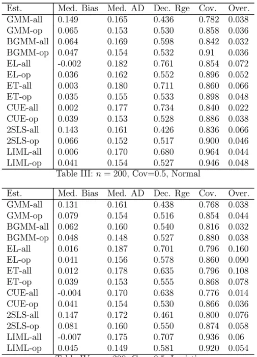
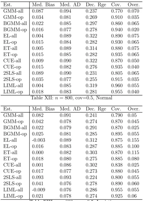
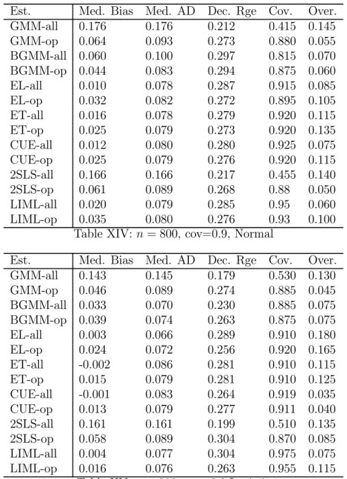
For each model experiments were conducted with the specifications for sample sizes of n = 200 and n = 1000. When the sample size is 200 we set R2

f = 0.1, ¯K = 10 and

performed 500 replications, while in the larger sample size we set R2

f = 0.1, ¯K = 20 and

we performed 200 replications (due to time constraints). Both of these choices reflect the fairly common situation where there may be a relatively small amount of correlation between the instruments and the endogenous variable (see Staiger and Stock (1997) and Stock and Wright (2000) as well as the fact that with larger data sets empirical researchers are more willing to use more moment conditions to improve efficiency. For each of these cases we consider c _{∈ {.1, .5, .9}, though for brevity we will only report} results for c = .5. In addition we consider the impact of having excess kurtosis, which as noted above has differential effect on the higher order MSE across the different estimators. The distribution we consider is that of

µ ρi ηi ¶ =_|ei| µ ρ∗ i ηi∗ ¶ , µ ρ∗ i ηi∗ ¶ ∼ N(0, Σ), ei ∼ logistic(0,1).

where ei is independent of ρ∗i and ηi∗ and is distributed as a logistic random variable

with mean zero and variance equal to one. Given this particular setup we will have that (ρi, ηi) are jointly distributed with mean zero and a covariance matrix equal to Σ, and a

coefficient of kurtosis of approximately κ = 12.6. With two different models, two different distributions for the errors, and three different choices for residual correlations there are a total of 12 specifications for each sample size.

The estimator that uses all moments or instruments is indicated by the suffix “-all” while the estimator that uses a number of moment conditions as chosen by the respective moment or instrument selection criterion is indicated by “-op”. Therefore, for instance, GMM-all and GMM-op are the two step estimator that uses all of the moment conditions and the moment conditions the minimize the estimated MSE criterion respectively. The preliminary estimates of the objects that appear in the criteria were in each case based on a number of moment conditions that was optimal with respect to cross validation in the first stage.

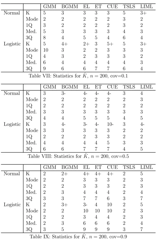
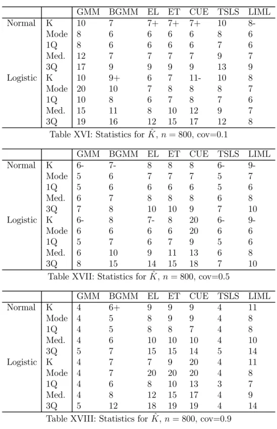
As in Donald and Newey (2001) we present robust measures of central tendency and dispersion. We computed the median bias (Med. Bias) for each estimator, the median of the absolute deviations (MAD) of the estimator from the true value of γ = 0 and examined dispersion through the difference between the 0.1 and 0.9 quantile (Dec. Rge) in the distribution of each estimator. We also examined statistical inference by computing the coverage rate for 95% confidence intervals as well as the rejection rate for an overidentification test (in cases where overidentifying restrictions are present) using the test statistic corresponding to the estimator and a significance level of 5%. In addition we report some summary statistics concerning the choices of K in the experiments, including the modal choice of K if one used the actual MSE to choose K. There was very little dispersion in this variable across replications and generally the optimal K with the true criterion was equal to the same value in most if not all replications. In cases where there was some dispersion it was usually either being some cases on either side of the mode. To indicate such cases we use + and -, so that for instance 3+ means that the mode was 3 but that there were some cases where 4 was optimal. The notation 3++ means that the mode was 3 but that a good proportion of the replications had 4 as being optimal.

Tables I-VI and X-XV contains the summary statistics for the estimators for n = 200 and n = 800 respectively, while Tables VII-IX and XVI-XVIII contain the summary statistics for the chosen number of moments across the replications. In general the results are encouraging for all the estimators. As expected the GEL and LIML estimators are less dispersed when the optimal number of moments is used, while for GMM and 2SLS

the use of the criterion reduces the bias that occurs when there is a high degree of covariance between the residuals. The improvements for the GEL estimators are more marked when the there is a low to moderate degree of covariance. It is noteworthy that in such situations there is also a dramatic improvement in the quality of inference as indicated by the coverage rates for the confidence interval. As far as testing the overidentifying restrictions only when there is a high degree of covariance is there any problem with testing these restrictions. This occurs with most of the estimators in the small sample with a high covariance and with GMM and TSLS in the large sample with a high covariance. It also seems that using the criteria does not really help in fixing any of these problems.

There are a number of things to note about the results for ˆK. First, the estimated criteria give values for ˆK that are often near the values that minimize the true criterion, suggesting that the estimated criterion is a good approximation to the true criterion. It also noteworthy that, as one would expect, the criteria suggest use of a small number of moments for GMM and 2SLS when there is a high error covariance and for the GEL estimators when there is a low covariance. For BGMM the optimal number is quite stable as the covariance increases. In the larger sample the optimal number decreases as the covariance increases, but is slightly larger when the residuals have fat tails compared to the situation where they do not. Among the GEL estimators increasing the covariance and having fat tailed errors has the most dramatic impact on CUE as one would expect given the criteria.

Concerning the effect of excess kurtosis, it does appear that the improvement from using the criteria is more noticeable for EL, which is most sensitive to having fat tailed errors. There also was some evidence that going from normal to fat tailed errors helped CUE more than the other estimators, as suggested in the theory, although this led to a lower improvement from using the moment selection criterion.

5

Conclusion

In this paper we have developed approximate MSE criteria for moment selection for a variety of estimators in conditional moment contexts. We found that the CUE has smaller MSE than the bias corrected GMM estimator. In addition we proposed data based methods for estimating the approximate MSE, so that in practice the number of moments can be selected by minimizing these criteria. The criteria seemed to perform adequately in a small scale simulation exercise.

The present paper has considered a restrictive environment in which the data are considered a random sample. It would be useful to extend the results in two directions. The first would be to the dynamic panel data case. In that situation there will typically be different sets of instruments available for each residual coming from sequential moment restrictions. It would also be useful to extend the results to a purely time series context where one would need to deal with serial correlation. Kuersteiner (2002) has derived interesting results in this direction.

Appendix A: MSE Derivation Results

Throughout the Appendix repeated use of the Cauchy Schwarz (CS), Markov (M) and Triangle inequalities is made. We let _{k.k denote the usual matrix norm. The following} Maximum Eigenvalue (ME) inequality is also used repeatedly,

kA0BC_{k ≤ λ}max(BB)kAk kCk

for a square symmetric matrix B and conformable matrices A and C. For simplicity of notation and without loss of generality we assume that the true value of the coefficients are all zero and we only perform the calculation for the case where there is one parameter (in addition to the auxiliary parameters λ). Because higher order derivatives are required for the MSE calculations (even though they do not appear in the final result) we use the following notation: for j = 0, 1, ..., 4 we let,

Γj = 1 n X i Γji, ¯Γj = 1 n X i Γji(0), ˆΓj = 1 n X i Γji( ˆβ) Γji = qiE( ∂j+1 ∂βj+1ρi(0)|xi), Γji(β) = qi ∂j+1 ∂βj+1ρi(β) ηji = ∂j+1 ∂βj+1ρi(0)− E( ∂j+1 ∂βj+1ρi(0)|xi) and ¯Γ∗

j denotes ¯Γj evaluated at some point(s) lying between the respective estimator

and its true value. Hence Γ0 corresponds to Γ in the text. In addition we assume as in

Donald, Imbens and Newey (2003) (hereafter DIN) that qi has been normalized so that

kqik < Cζ(K) and E(qiqi0) = IK so that,

1 n X i kqik 2 = O(K), λmax( Ã 1 n X i qiqi0δi !2 ) = O(1), if δi < C <∞ λmin( 1 n X i qiqi0δi) > 0, for 0 < c < δi < C <∞

where here and elsewhere we let c denote a generic small constant and C a generic large constant. The MSE are based on an expansion that is contained in Appendix B. The remainder term for GEL is dealt with in a technical appendix that is available on request.

Derivatives that are used in the expansion are also available in a technical appendix that is available on request.

Proof of Proposition 1:

In deriving the MSE for GMM we simplify notation and refer to the estimator as ˆ

β as distinct from the preliminary estimator. Since we need the results for BGMM we expand the estimator and display all terms that are needed to perform the calculations in Proposition 2. Terms that will not be needed for GMM and BGMM are those that are o(K2/n3/2) and o(K/n3/2) respectively. Now for GMM we have from Newey and Smith (2004) (hereafter NS) we have that GMM can be written as the solution to the First Order Conditions, 1 n X i ∂ ∂βρi( ˆβ)q 0 iλ = 0ˆ 1 n X i qiρi( ˆβ) + ˆΥ( ˜β)ˆλ = 0 where by DIN ° ° °ˆλ°°° = O(pK/n) and ° ° ° ˆβ ° °

° = O(1/√n). Using Appendix B and the partitioned inverse formula applied to

M−1 = µ 0 Γ0 0 Γ0 Υ−1 ¶−1 = µ −Ω−1 _Ω−1_Γ0 0Υ−1 Υ−1_Γ 0Ω−1 Σ ¶ where Ω = Γ0

0Υ−1Γ0 and Σ = Υ−1− Υ−1Γ0Ω−1Γ00Υ−1 we have that,

−M−1m = µ −Ω−1Γ00Υ−1g¯ −Σ¯g ¶ = µ T₁β Tλ 1 ¶

Note that we have_kΩ−1_{k = O(1), kΥ}−1_Γ

0k = O(1) by ME kΓ0k = O(1) and λmax(Υ−1) =

O(1) and finally, λmax(Σ) ≤ λmax(Υ−1) = O(1). Similarly by Appendix B and the

tech-nical appendix, −M−1( ˆM _{− M)θ =} ⎛ ⎝ Ω−1 ¡_¯ Γ0− Γ0 ¢0_ˆ λ_{− Ω}−1_Γ0 0Υ−1 ³³ ˆ Υ( ˜β)_{− Υ}´ˆλ +¡Γ¯0− Γ0 ¢ _ˆ β´ −Υ−1Γ0Ω−1 ¡_¯ Γ0− Γ0 ¢0_ˆ λ_{− Σ}³¡Γ¯0− Γ0 ¢ _ˆ β + ³ ˆ Υ( ˜β)_{− Υ} ´ ˆ λ ´ ⎞ ⎠ = µ T₂β T2λ ¶ = µ

O(K/n) + O(K/n) + O(1/n) O(K/n) + O(√K/n) + O(ζ(K)K/n) ¶ µ T₃β Tλ 3 ¶ =_−M−1X j θjAjθ/2 = µ Ω−1βΓˆ 01λˆ− (1/2)Ω−1Γ00Υ−1βˆ2Γ1 −Υ−1_Γ 0Ω−1βΓˆ 01λˆ− (1/2)Σ ˆβ2Γ1 ¶ = µ O(1/n) O(1/n) ¶

−M−1X j θj( ˆAj− Aj)θ = µ Ω−1βˆ¡Γ¯1 − Γ1 ¢0_ˆ λ_{− (1/2)Ω}−1Γ00Υ−1βˆ2 ¡_¯ Γ1− Γ1 ¢ −Υ−1_Γ 0Ω−1βˆ ¡_¯ Γ1− Γ1 ¢0_ˆ λ_{− (1/2)Σ ˆ}β2¡_Γ¯ 1− Γ1 ¢ ¶ = µ T₄₁β + T₄₂β T41λ + T42λ ¶ = µ O(K/n3/2_{) + O(}√_K/n3/2₎ O(K/n3/2_{) + O(}√_K/n3/2₎ ¶

Next we have that, µ T₅β T5λ ¶ = _−M−1X j X k θjθkBjkθ/6 =−(1/6) µ −Ω−1_{3 ˆβ}2_Γ0 2λ + Ωˆ −1Γ00Υ−1βˆ3Γ2 Υ−1_Γ 0Ω−13 ˆβ2Γ02λ + Σ ˆˆ β3Γ2 ¶ = ⎛ ⎝ O( ° ° ° ˆβ ° ° °2kΓ2k ° ° °ˆλ°°°) O( ° ° ° ˆβ ° ° ° 3 kΓ2k) ⎞ ⎠ = µ O(√K/n3/2₎ O(1/n3/2₎ ¶

by CS, the results for ° ° ° ˆβ ° ° ° and ° ° °ˆλ ° °

° , Assumption 3, and the conditions on the elements of M−1_{. Next we have,} X j X k θjθk ³ ˆ Bjk− Bjk ´ θ/6 = (1/6) µ 3 ˆβ2¡Γ¯2− Γ2 ¢0_ˆ λ ˆ β3¡_Γ¯ 2− Γ2 ¢ ¶ = ⎛ ⎜ ⎝ Oµ°°_{° ˆ}β°°_°2°°¯Γ2− Γ2 ° °°°_°ˆλ°°_°¶ O( ° ° ° ˆβ ° ° ° 3° °¯Γ2− Γ2 ° °) ⎞ ⎟ ⎠ = µ O(K/n2₎ O(√K/n2₎ ¶

The last term is (1/24) times, X j X k θjθk X l θlCˆjklθ = Ã ˆ β4³_Γ¯∗0 4λˆ ´ + 4 ˆβ3_Γ¯∗0 3λˆ ¯ Γ∗ 3βˆ4 ! = ⎛ ⎜ ⎝ O( ° ° ° ˆβ ° ° °3°°°ˆλ°°° (°°° ˆβ ° ° °°°¯Γ∗ 4 ° ° +°°¯Γ∗ 3 ° °) Oµ°°¯Γ∗ 3 ° °°°_{° ˆ}β°°_°4 ¶ ⎞ ⎟ ⎠ = O(√K/n2) Therefore, ° ° °Rβn,K ° ° ° = O(K/n2_{) and} °° °Rβn,K ° °

° = O(K/n2_{) by CS and ME and the}

condi-tion on the elements of M−1_{. Here we have used} °°Γ0 0Υ−1 ¡_¯ Γ0− Γ0¢°° = O(1/√n) and ° ° °Γ0 0Υ−1 ³ ˆ

Υ( ˜β)_{− Υ}´°°_{° = O(}pK/n + ζ(K)/√n) = O(ζ(K)/√n) which follow from DIN Lemma A4.

Note that by Assumption 2 we can write, ˆ

Υ( ˜β)_{− Υ = ˆ}Υv1+ 2 ˜βΥρη+ 2 ˜β ˆΥv2+ 2 ˜β ˆΥv3+ ˜β2Υˆr

where, ˆ Υvj = 1 n X i qiqi0vji for j = 1, 2, 3 E(vji|xi) = 0 v1i = ρ2i − σ 2 i, v2i= diρi, v3i = (η0iρi− σρη(xi)) Υρη = 1 n X i qiqi0σρη(xi), ˆΥr = 1 n X i qiqi0ri

and E(vji|xi) = 0, E(v2ji|xi) < C Assumption 1.E(krik |xi) < C by Assumption 2. Hence,

we have that, ° ° ° ˆΥvj ° ° ° = O(ζ(K)pK/n), ° ° ° ˆRΥn,K ° ° ° = O³(ζ(K)√K + K)/n´ λmax(ΥρηΥρη) = O(1), λmax( ˆΥrΥˆr) = O(1)

° ° ° ˆΥvjΣ¯g ° ° ° = O(ζ(K)√K/n) for j = 1, 3 ° ° ° ˆΥvjΣ ¡_¯ Γ0− Γ0¢°°° = O(ζ(K) √ K/n) for j = 1, 3 ° ° ° ˆΥv2Σ¯g ° ° ° = O(ζ(K)K/n), ° ° ° ˆΥv2Σ ¡_¯ Γ0 − Γ0¢°°° = O(ζ(K)K/n) ° ° °Γ0Υ−1ΥˆvjΣ ° ° ° = O(pK/n), °°Γ0Υ−1ΥρηΣ ° ° = O(1),°°_°Γ0Υ−1ΥˆrΣ ° ° ° = O(1) ° °¯Γ0− Γ0 ° ° = O(pK/n), ° ° °¡Γ¯0 − Γ0 ¢0 Υ−1Γ0 ° ° ° = O(1/√n)

with the last fact following from M and Assumptions 1 and 3. For the ˆλ terms from the above expansion it follows that,

ˆ λ =_{−Σ¯g − Υ}−1Γ0Ω−1 ¡_¯ Γ0− Γ0 ¢0_ˆ λ_{− Σ}¡Γ¯0− Γ0 ¢_ˆ β_{− Σ}³Υ( ˜ˆ β)_{− Υ}´ˆλ + Rλ₁ where °°Rλ 1 °

° = O(1/n) under the condition on K for GMM and hence for BGMM also. Repeated substitution and using the facts that by CS and the results for ˆλ and°°¯Γ0 − Γ0

° ° and the fact that from the above expansion ˆβ =_−Ω−1Γ00Υ−1g+R¯

β 1 with ° ° °R1β ° ° ° = O(K/n), ˆ λ =_{−Σ¯g + Υ}−1Γ0Ω−1 ¡_¯ Γ0− Γ0 ¢0 Σ¯g + Σ¡Γ¯0− Γ0 ¢ Ω−1Γ00Υ−1g¯ +Σ ˆΥvjΣ¯g + 2 ˜βΣΥρηΣ¯g + Rλ2, ° ° °Υ−1Γ0Ω−1 ¡_¯ Γ0− Γ0 ¢0 Σ¯g°°_{° = O(K/n)}°°Σ ¡¯Γ0 − Γ0 ¢ Ω−1Γ0₀Υ−1g¯°° = O(√K/n) ° ° °Σ ˆΥvjΣ¯g ° ° ° = O(ζ(K)√K/n), ° ° °2 ˜βΣΥρηΣ¯g ° ° ° = O(√K/n), ° °Rλ 2 ° ° = O(ζ(K)√K/n)O(ζ(K)pK/n)

where°°Rλ2

°

° = o(√K/n) under the condition on K for BGMM and°°R2λ

°

° = O(1/√n)o(ζ(K)K/n) = O(1/√n)o(K2_{/n) under the condition on K for GMM.}

Take the lead term in the expansion for ˆβ, T₂β and substitute in for ˆλ and apply CS, and M to get that,

Ω−1¡Γ¯0 − Γ0 ¢0_ˆ λ = _−Ω−1¡Γ¯0− Γ0 ¢0 Σ¯g + Ω−1¡Γ¯0− Γ0 ¢0 Υ−1Γ0Ω−1 ¡_¯ Γ0− Γ0 ¢0 Σ¯g +Ω−1¡Γ¯0− Γ0 ¢0 Σ¡Γ¯0− Γ0 ¢ Ω−1Γ0₀Υ−1g¯ +Ω−1¡Γ¯0− Γ0 ¢0 Σ ˆΥv1Σ¯g + 2 ˜βΩ−1 ¡_¯ Γ0− Γ0 ¢0 ΣΥρηΣ¯g + R β 2 Rβ₂ = _−Ω−1¡Γ¯0− Γ0 ¢0 Rλ₂ Here ° ° °R2β ° °

° = O(pK/n)o(√K/n) = O(1/√n)o(K/n) under the condition for BGMM, and −Ω−1¡Γ¯0− Γ0 ¢0 Σ¯g = O(K/n) Ω−1¡Γ¯0− Γ0 ¢0 Σ¡Γ¯0− Γ0 ¢ Ω−1Γ0₀Υ−1g = O(1/¯ √n)O(K/n) Ω−1¡Γ¯0− Γ0 ¢0 Υ−1Γ0Ω−1 ¡_¯ Γ0− Γ0 ¢0 Σ¯g = O(1/√n)O(K/n) Ω−1¡Γ¯0− Γ0 ¢0 Σ ˆΥv1Σ¯g = O(1/ √ n)O(ζ(K)K/n) 2 ˜βΩ−1¡Γ¯0− Γ0 ¢0 ΣΥρηΣ¯g = O(1/ √ n)O(K/n) Under the condition on K for GMM we have,

−Ω−1¡Γ¯0− Γ0 ¢0_ˆ λ =−Ω−1¡Γ¯0− Γ0 ¢0 Σ¯g + Ω−1¡Γ¯0− Γ0 ¢0 Σ ˆΥv1Σ¯g + Rβ3

where°°_°Rβ₃°°_{° = O(1/}√n)o(K2_/n).

Now consider the second term in T₂β given by _−Ω−1_Γ0 0Υ−1

³ ˆ

Υ( ˜β)_{− Υ}´λ. Using theˆ facts above we can write,

−Ω−1Γ0₀Υ−1³Υ( ˜ˆ β)_{− Υ}´ = _−Ω−1Γ0₀Υ−1Υˆv1− 2 ˜βΩ−1Γ00Υ−1Υρη− 2 ˜βΩ−1Γ00Υ−1Υˆv2+ o( √ K/n) ° ° °−Ω−1Γ0₀Υ−1Υˆv1 ° ° ° = O(pK/n), ° ° °2 ˜βΩ−1Γ0₀Υ−1Υρη ° ° ° = O(1/√n), ° ° °2 ˜βΩ−1Γ00Υ−1Υˆv2 ° ° ° = O(√K/n)

so that using the above expansion for ˆλ and repeated use of CS and M, −Ω−1Γ0₀Υ−1³Υ( ˜ˆ β)_{− Υ}´ˆλ = Ω−1Γ₀0Υ−1Υˆv1Σ¯g + 2 ˜βΩ−1Γ00Υ−1ΥρηΣ¯g +2 ˜βΩ−1Γ0₀Υ−1Υˆv2Σ¯g− Ω−1Γ00Υ−1Υˆv1Υ−1Γ0Ω−1 ¡_¯ Γ0− Γ0 ¢0 Σ¯g −2 ˜βΩ−1Γ00Υ−1ΥρηΥ−1Γ0Ω−1 ¡_¯ Γ0− Γ0 ¢0 Σ¯g −Ω−1Γ0₀Υ−1Υˆv1Σ ˆΥv1Σ¯g− 2 ˜βΩ−1Γ00Υ−1ΥρηΣ ˆΥv1Σ¯g −2 ˜βΩ−1Γ0₀Υ−1Υˆv1ΣΥρηΣ¯g + Rβ ° °Rβ°_{° = O(}p K/n)O(°°Rλ2 ° °) using the fact that also under the Assumption 1,

° ° °−Ω−1Γ0₀Υ−1Υˆv1Σ ¡_¯ Γ0− Γ0 ¢ Ω−1Γ0₀Υ−1g¯ ° ° ° = O(1/√n)O(√K/n) Here we have that,

° ° °Ω−1Γ0₀Υ−1Υˆv1Σ¯g ° ° ° = O(1/√n)O(pK/n) ° ° °2 ˜βΩ−1Γ0₀Υ−1ΥρηΣ¯g ° ° ° = O(1/√n)O(1/√n) ° ° °2 ˜βΩ−1Γ00Υ−1Υˆv2Σ¯g ° ° ° = O(1/√n)O(K/n) ° ° °Ω−1Γ0₀Υ−1Υˆv1Υ−1Γ0Ω−1 ¡_¯ Γ0− Γ0 ¢0 Σ¯g°°_{° = O(1/}√n)O(K/n) ° ° °2 ˜βΩ−1Γ00Υ−1ΥρηΥ−1Γ0Ω−1 ¡_¯ Γ0− Γ0 ¢0 Σ¯g ° ° ° = O(1/√n)O(K/n) Ω−1Γ0₀Υ−1Υˆv1Σ ˆΥv1Σ¯g = O( p

K/n)O(ζ(K)√K/n) = O(1/√n)O(ζ(K)K/n) 2 ˜βΓ0₀Υ−1ΥρηΣ ˆΥv1Σ¯g = O(1/ √ n)O(ζ(K)√K/n) 2 ˜βΩ−1Γ0₀Υ−1Υˆv1ΣΥρηΣ¯g = O(1/ √ n)O(K/n)

and under the condition on K for BGMM °°Rβ°° = O(1/√n)o(K/n). So under the con-ditions for GMM we have that°°Rβ°° = O(1/√n)o(K2_{/n) and that by the above results,}

−Ω−1Γ00Υ−1

³ ˆ

Υ( ˜β)_{− Υ}´ˆλ = Ω−1Γ00Υ−1Υˆv1Σ¯g + 2 ˜βΩ−1Γ00Υ−1ΥρηΣ¯g

with ° ° °Rβ3 ° ° ° = O(1/√n)o(K2_/n).

Now take the third term in T₂βand using the above results and the fact that ° ° °−Ω−1_Γ0 0Υ−1 ¡_¯ Γ0− Γ0 ¢_ˆ β ° ° ° O(1/n) we have that

ˆ β =_−Ω−1Γ0₀Υ−1g¯_{− Ω}−1¡Γ¯0− Γ0 ¢0 Σ¯g + o(K/n) so, −Ω−1Γ00Υ−1 ¡_¯ Γ0− Γ0 ¢ _ˆ β = Ω−1Γ00Υ−1 ¡_¯ Γ0− Γ0 ¢ Ω−1Γ00Υ−1g¯ +Ω−1Γ0₀Υ−1¡Γ¯0− Γ0 ¢ Ω−1¡Γ¯0− Γ0 ¢0 Σ¯g + O(1/√n)o(K/n) under the conditions for BGMM and

−Ω−1Γ00Υ−1 ¡_¯ Γ0− Γ0 ¢ _ˆ β = Ω−1Γ00Υ−1 ¡_¯ Γ0− Γ0 ¢ Ω−1Γ00Υ−1g + O(1/¯ √ n)o(K2/n) under the conditions for GMM where,

° °Ω−1_Γ0 0Υ−1 ¡_¯ Γ0 − Γ0 ¢ Ω−1Γ0₀Υ−1g¯°° = O(1/√n)O(1/√n) ° ° °Ω−1Γ0₀Υ−1¡Γ¯0− Γ0 ¢ Ω−1¡Γ¯0− Γ0 ¢0 Σ¯g°°_{° = O(1/}√n)O(K/n) Next we have for T3β by the above expansion for ˆλ,

Γ0₁λ =ˆ _−Γ0₁Σ¯g_{− Γ}0₁Υ−1Γ0Ω−1 ¡_¯ Γ0− Γ0 ¢0 Σ¯g + Γ0₁Σ¡Γ¯0− Γ0 ¢ Ω−1Γ0₀Υ−1g¯ +Γ0₁Σ ˆΥv1Σ¯g + 2 ˜βΓ01ΣΥρηΣ¯g + Γ01R λ 2, By showing that ° ° °Γ0 1Σ ˆΥv1Σ¯g ° °

° = O(√K/n) and _kΓ01ΣΥρηΣ¯gk = O(1/√n) we can show

that under the condition for BGMM

Γ01λ =ˆ −Γ01Σ¯g− Γ01Υ−1Γ0Ω−1

¡_¯ Γ0− Γ0

¢0

Σ¯g + o(K/n) so that, after substituting in for ˆβ we have,

Ω−1βΓˆ 0₁λˆ_{− (1/2) ˆ}β2Ω−1Γ0₀Υ−1Γ1 = Ω−1Γ01Σ¯gΩ−1Γ00Υ−1g¯− Γ01Υ−1Γ0Ω−1 ¡_¯ Γ0− Γ0 ¢0 Σ¯gΩ−1Γ00Υ−1¯g +Ω−1Γ0₁Σ¯gΩ−1¡Γ¯0 − Γ0 ¢0 Σ¯g_{− (1/2)Ω}−1Γ0₀Υ−1Γ1 ¡ Ω−1Γ0₀Υ−1¯g¢2 −Ω−1Γ0₀Υ−1Γ1Ω−1Γ00Υ−1gΩ¯ −1 ¡_¯ Γ0− Γ0 ¢0 Σ¯g + O(1/√n)o(K/n)

where Ω−1Γ01Σ¯gΩ−1Γ00Υ−1¯g = O(1/ √ n)O(1/√n) Γ0₁Υ−1Γ0Ω−1 ¡_¯ Γ0− Γ0 ¢0 Σ¯gΩ−1Γ0₀Υ−1¯g = O(1/√n)O(K/n) Ω−1Γ0₁Σ¯gΩ−1¡Γ¯0 − Γ0 ¢0 Σ¯g = O(1/√n)O(K/n) (1/2)Ω−1Γ00Υ−1Γ1 ¡ Ω−1Γ00Υ−1g¯ ¢2 = O(1/n) Ω−1Γ0₀Υ−1Γ1Ω−1Γ00Υ−1¯gΩ−1 ¡_¯ Γ0 − Γ0 ¢0 Σ¯g = O(1/√n)O(K/n) For the term T₄β we have,

T4β = (1/2)2 ˆβΩ−1(¯Γ1− Γ1)0ˆλ + O(1/ √ n)o(K/n) = Ω−1(¯Γ1− Γ1)0Σ¯gΩ−1Γ00Υ−1g + O(1/¯ √ n)o(K/n) ° °Ω−1¡_(¯Γ 1− Γ1)0Σ¯g ¢ Ω−1Γ0₀Υ−1g¯°° = O(1/√n)O(K/n) Finally we note that we have

° ° °T5β

° °

° = O(1/√n)o(K/n) so that we have now found all terms that are the right order.

For GMM let γK,n= K2/n + ∆K,n with ∆K,n = Ω∗− Ω. Then by,

n³ζ(K)K/n3/2+√K/n + 1/n´

2

= o(K2/n)

n³ζ(K)K/n3/2+√K/n + 1/n´K/√n = O(ζ(K)/√n)O(K2/n) = o(K2/n) so with h =_−Γ0 0Υ−1g, we can write,¯ √ n ˆβH = √nΩ−1(h + 4 X j=1 T_jH+ ZH) ° °TH 1 ° ° = O(K/√n), °°TH 2 ° ° = O(pK/n), °°T₃H°° = O(1/√n) ° °TH 4 ° ° = O(ζ(K)K/n),°°ZH°_{° = o(K}2_/n)

Using the expansion, Ω−1 _{= Ω}∗−1_{+ Ω}∗−1_(Ω∗_{− Ω) Ω}∗−1_{+ O(∆}2

K,n) and noting that under

the condition on K, TH

1 = o(1) then we can write,

³√ n ˆβH´ 2 = nΩ−1hh0Ω−1+ Ω∗−1 Ã T1HT H 1 + 2 4 X j=1 hTjH ! Ω∗−1+ o(γK,n)

Ω−1E(hh0)Ω−1 = Ω−1 = Ω∗−1+ Ω∗−1(Ω∗_{− Ω) Ω}∗−1+ O(∆2_K,n) with E¡hTH

1

¢

= E(hTH

2 ) = 0 by the third moment condition. Next,

E¡nT1HT1H ¢ = 1 n à X i E(ρiη0i)ξii !2 + o(γK,n)

and by the third moment condition,

nE(T₁Hh) = nE(Γ0₀Υ−1Υˆv1Σ¯gh) = 1 n X i (κi− 1)d2iξii+ o(γK,n) = O(K/n) = o(γK,n) nE(T₃Hh) = _−nE(¡Γ¯0− Γ0 ¢0 Σ ˆΥv1Σ¯gh) + nE(Γ00Υ−1Υˆv1Σ ˆΥv1Σ¯gh) −2nE( ˜βΓ0₀Υ−1ΥρηΣ ˆΥv1Σ¯g) = ₋1 n X i (κi− 1)d2iξii+ o(γK,n)

Therefore we have the result,

E(ntΩ−1³h2+ 2hT_h1+¡T_h1¢2+ 2hT_h2´Ω−1t) = Ω∗−1+ Π2/n +¡Ω∗_{− Γ}0₀Υ−1Γ0

¢

+ o(γK,n)

using the fact that Ω∗_Ω−1 _{= I + (Ω}∗_{− Ω) Ω}∗−1_{+ O(∆}2

K,n) and the fact that τ = Ω∗t

Proof of Proposition 2: For BGMM we have the additional term, (ˆΓ0₀Υˆ−1Γˆ0)−1 n X i=1 ˆ Γ0_0iΣˆˆgi/n2 = ˆΩ−1 n X i=1 ˆ Γ0_0iΣˆˆgi/n2 ˆ Γ0 = n X i=1 ˆ Γ0i/n, ˆΓ0i= qiyˆi, ˆyi = [∂ρi( ˆβH)/∂β]0, ˆgi = qiρi( ˆβH) ˆ Σ = Υˆ−1_{− ˆ}Υ−1Γˆ0Ωˆ−1Γˆ00Υˆ−1, ˆΩ = ˆΓ00Υˆ−1Γˆ0

First we have by Assumption 3, letting Γ0i = qiE(∂ρi(0)/∂β), Γ0i(0) = qi∂ρi(0)/∂β

ˆ Γ0i = Γ0i+ (Γ0i(0)− Γ0i) + ˆβΓ1i+ ˆβ(Γ1i(0)− Γ1i) + ³ ˆ β´ 2 Γ∗2i ˆ gi = gi+ Γ0iβ + (Γˆ 0i(0)− Γ0i) ˆβ + ³ ˆ β´ 2 Γ∗_1i

Using, ˆ Ω−1 = Ω−1+ Ω−1³Ω_{− ˆ}Ω´Ω−1+ Ω−1³Ω_{− ˆ}Ω´Ωˆ−1³Ω_{− ˆ}Ω´Ω−1 and, ˆ Ω_{− Ω = ˆ}Γ0₀Υˆ−1Γˆ0− ˆΓ00Υ−1Γˆ0+ ˆΓ00Υ−1Γˆ0− Γ00Υ−1Γ0 ˆ Γ00Υˆ−1Γˆ0− ˆΓ00Υ−1Γˆ0 = Γ00 ³ ˆ Υ−1_{− Υ}−1´Γ0+ ³ ˆ Γ0− Γ0 ´0³ ˆ Υ−1_{− Υ}−1´Γ0 +Γ0₀³Υˆ−1_{− Υ}−1´ ³Γˆ0− Γ0 ´ +³Γˆ0− Γ0 ´0³ ˆ Υ−1_{− Υ}−1´ ³Γˆ0− Γ0 ´ with ˆ Γ0− Γ0 = ¯Γ0 − Γ0 + ˆβ ¯Γ1+ ˆβ2Γ¯∗1 = ¯Γ0 − Γ0 + ˆβΓ1+ ˆβ(¯Γ1− Γ1) + ˆβ2Γ¯∗1 we can write, ³ ˆ Υ−1_{− Υ}−1´ = Υ−1³Υ_{− ˆ}Υ´Υ−1+ Υ−1³Υ_{− ˆ}Υ´Υˆ−1³Υ_{− ˆ}Υ´Υ−1 Γ00 ³ ˆ Υ−1_{− Υ}−1´Γ0 = Γ00Υ−1 ³ Υ_{− ˆ}Υ´Υ−1Γ0 +Γ0₀Υ−1³Υ_{− ˆ}Υ´Υˆ−1³Υ_{− ˆ}Υ´Υ−1Γ0 Γ0₀Υ−1³Υ_{− ˆ}Υ´Υˆ−1³Υ_{− ˆ}Υ´Υ−1Γ0 = O(K/n) Γ00Υ−1 ³ Υ_{− ˆ}Υ´Υ−1Γ0 = −Γ00Υ−1Υˆv1Υ−1Γ0 − ˆβΓ0₀Υ−1ΥρηΥ−1Γ0+ O(1/n) Γ00Υ−1Υˆv1Υ−1Γ0 = O(1/√n) ˆ βΓ0₀Υ−1ΥρηΥ−1Γ0 = O(1/ √ n) ³ ˆ Γ0− Γ0 ´0³ ˆ Υ−1_{− Υ}−1´Γ0 = O(ζ(K) √ K/n) ³ ˆ Γ0− Γ0 ´0³ ˆ Υ−1_{− Υ}−1´ ³Γˆ0− Γ0 ´ = o(K/n) ˆ Γ0₀Υ−1Γˆ0− Γ00Υ−1Γ0 = ³ ˆ Γ0− Γ0 ´0 Υ−1Γ0 + Γ00Υ−1 ³ ˆ Γ0− Γ0 ´ + ³ ˆ Γ0 − Γ0 ´0 Υ−1 ³ ˆ Γ0− Γ0 ´ ³ ˆ Γ0− Γ0 ´0 Υ−1Γ0 = ¡_¯ Γ0− Γ0 ¢0 Υ−1Γ0 + ˆβΓ1Υ−1Γ0+ O(1/n) ³ ˆ Γ0− Γ0 ´0 Υ−1³Γˆ0− Γ0 ´ = O(K/n)

so that, ˆ Ω_{− Ω = Γ}0₀Υ−1Υˆv1Υ−1Γ0+ 2 ˆβΓ00Υ−1ΥρηΥ−1Γ0− ¡_¯ Γ0− Γ0 ¢0 Υ−1Γ0− ˆβΓ1Υ−1Γ0 −Γ00Υ−1 ¡_¯ Γ0− Γ0 ¢ − ˆβΓ00Υ−1Γ1 + O(ζ(K) √ K/n) ° ° °ˆΩ_{− Ω} ° ° ° = O(1/√n) Now, n X i=1 ˆ Γ00iΣˆˆgi/n2 = µ 1 n2 ¶_Xn i=1 ˆ Γ00iΣˆgi/n2+ µ 1 n2 ¶_Xn i=1 ˆ Γ00i( ˆΣ− Σ)ˆgi/n2 and, n X i=1 ˆ Γ0iΣˆgi/n2 = n X i=1 Γ0_0iΣgi/n2+ n X i=1 Γ0_0iΣΓ0iβ/nˆ 2+ n X i=1 (Γ0i(0)− Γ0i)0Σgi/n2 + n X i=1 (Γ0i(0)− Γ0i)0Σ (Γ0i(0)− Γ0i) ˆβ/n2 + ˆβ n X i=1 (Γ1i(0)− Γ1i)0Σgi/n2+ O(1/ √ n)o(K/n) with, n X i=1 Γ0_0iΣgi/n2 = O(1/ √ n)O(ζ(K)√K/n) n X i=1 Γ00iΣΓ0iβ/nˆ 2 = O(1/ √ n)O(K/n) n X i=1 (Γ0i(0)− Γ0i)0Σgi/n2 = O(1/ √ n)O(K/√n) n X i=1 (Γ0i(0)− Γ0i)0Σ (Γ0i(0)− Γ0i) ˆβ/n2 = O(1/√n)O(K/n) ˆ β n X i=1 (Γ1i(0)− Γ1i)0Σgi/n2 = O(1/√n)O(K/n)

Next n X i=1 ˆ Γ0_0i( ˆΣ_{− Σ)ˆg}i/n2 = n X i=1 ˆ Γ0_0i³Υˆ−1_{− Υ}−1´ˆgi/n2 + n X i=1 ˆ Γ0_0i³Υ−1Γ0Ωˆ−1Γˆ00Υˆ−1− ˆΥ−1Γˆ0Ω−1Γˆ00Υˆ−1 ´ ˆ gi/n2 + n X i=1 ˆ Γ0_0i³Υˆ−1Γˆ0Ω−1Γˆ00Υˆ−1− Υ−1Γ0Ω−1Γ00Υ−1 ´ ˆ gi/n2

For the first term using the above expansions for ˆΥ−1_−Υ−1 _{and for Υ− ˆΥ in Proposition}

1, we can show that using T, followed by CS and then ME and the conditions on K, for BGMM we have n X i=1 ˆ Γ00iΥ−1 ³ Υ_{− ˆ}Υ´Υ−1ˆgi/n2 =− n X i=1 Γ00iΥ−1Υˆv1Υ−1gi/n2− n X i=1 (Γ0i(0)− Γ0i)0Υ−1Υˆv1Υ−1gi/n2 −2 ˆβ n X i=1 (Γ0i(0)− Γ0i)0Υ−1ΥρηΥ−1gi/n2 + O(1/√n)o(K/n) with, ° ° ° ° ° n X i=1 Γ0_0iΥ−1Υˆv1Υ−1gi/n2 ° ° ° ° ° = (1/ √ n)O(ζ(K)K/n) ° ° ° ° ° n X i=1 (Γ0i(0)− Γ0i)0Υ−1Υˆv1Υ−1gi/n2 ° ° ° ° ° = (1/ √ n)O(ζ(K)K/n) ° ° ° ° °2 ˆβ n X i=1 (Γ0i(0)− Γ0i)0Υ−1ΥρηΥ−1gi/n2 ° ° ° ° °= O(1/ √ n)O(K/n) where the second part of the first term satisfies (using similar arguments),

° ° ° ° ° n X i=1 ˆ Γ0_0iΥ−1³Υ_{− ˆ}Υ´Υˆ−1³Υ_{− ˆ}Υ´Υ−1gˆi/n2 ° ° ° ° °= O(1/ √ n)o(K/n)

For the remaining terms we can show using similar arguments that they are each O(1/√n)o(K/n). So altogether Pn_i=1Γˆ0iΣˆˆgi/n2 = O(K/√n) so that by the condition on K and,

O(K/√n)³O(ζ(K)√K/n) + O(∆K,n)

´

we have that ˆ Ω−1 n X i=1 ˆ Γ0_0iΣˆˆgi/n2 = Ω−1 n X i=1 Γ0_0iΣgi/n2+ Ω−1 n X i=1 Γ0_0iΣΓ0iβ/nˆ 2 +Ω−1 n X i=1 (Γ0i(0)− Γ0i)0Σgi/n2+ Ω−1 n X i=1 (Γ0i(0)− Γ0i)0Σ (Γ0i(0)− Γ0i) ˆβ/n2 +Ω−1βˆ n X i=1 (Γ1i(0)− Γ1i)0Σgi/n2− Ω−1 n X i=1 Γ0_0iΥ−1Υˆv1Υ−1gi/n2 −Ω−1 n X i=1 (Γ0i(0)− Γ0i)0Υ−1Υˆv1Υ−1gi/n2 −2 ˆβΩ−1 n X i=1 (Γ0i(0)− Γ0i)0Υ−1ΥρηΥ−1gi/n2 +Ω−1Γ00Υ−1Υˆv1Υ−1Γ0Ω−1 n X i=1 Γ00iΣgi/n2 +2 ˆβΩ−1Γ00Υ−1ΥρηΥ−1Γ0Ω−1 n X i=1 Γ00iΣgi/n2 −Ω−1³Γ0₀Υ−1¡Γ¯0− Γ0 ¢ +¡Γ¯0− Γ0 ¢0 Υ−1Γ´Ω−1 n X i=1 Γ0_0iΣgi/n2 − ˆβΩ−1¡Γ0₀Υ−1Γ1+ Γ1Υ−1Γ ¢ Ω−1 n X i=1 Γ0_0iΣgi/n2+ O(1/√n)o(K/n)

Now combining terms here with the terms that are not O(1/√n)o(K/n) from GMM and using the facts that for j = 0, 1,

−¡Γ¯j − Γj ¢0 Σ¯g + n X i=1 Γ0_0iΣgi/n2 = n X i6=j Γ0_0iΣgj/n2 = O(1/√n)O( p K/n)

and the fact that ˆβ =_−Ω−1_Γ0

0Υ−1g + o(1/¯

√

n) have that for instance, (¯Γ1− Γ1)0Σ¯gΩ−1Γ00Υ−1g + ˆ¯ β n X i=1 (Γ1i(0)− Γ1i)0Σgi/n2 = O(1/√n)O( √ K/n) This also occurs by combining terms from GMM and BGMM. Then for BGMM we have

that for γK,n = K/n + ∆K,n, √ n ˆβB = Ω−1(h + 5 X j=1 T_jB+ ZB) ° °TB 1 ° ° = O(pK/n), °°T₂B°° = O(ζ(K)K/n),°°T₃B°° = O(1/√n) ° °TB 4 ° ° = O(ζ(K)√K/n) °°T5B ° ° = O(K/n), °°ZB°_{° = o(γ} K,n)

then under the condition on K as with GMM, n³βˆB´2 = nΩ−1hh0Ω−1+ Ω∗−1(T₁BT₁B+

5

X

j=1

2T_jBh)Ω∗−1+ o(γK,n)

Now doing the calculations we get E(hTB

3 ) = O by Assumption 1(iv). Then we have for

E(TB 1 T1B) the terms, nE( n X i6=j Γ0_0iΣgj/n2) = 1 n X i E(η_0i2)ξii+ X i,j

E(ρiη0i)E(ρjη0j)ξ2ij+ o(γK,n)

nE(Γ0₀Υ−1Υˆv1Σ¯g n X i6=j Γ0_0iΣgj/n2) = o(γK,n) nE(Γ0₀Υ−1Υˆv1Σ¯g¯g0Σ ˆΥv1Υ−1Γ) = 1 n X i (κi− 1)d2iξii+ o(γK,n)

For the term 2T1Bh we have by Assumption 1(iv)

2nE(Γ0₀Υ−1Υˆv1Σ¯gh) =−2 1 n X i (κi− 1)d2iξii+ o(γK,n) Next for 2TB 2 h we have, −2nE(Γ00Υ−1Υˆv1Σ ˆΥv1Σ¯gh) = o(γK,n) −2nE(¡Γ¯0− Γ0 ¢0 Σ ˆΥv1Σ¯gh0) = o(γK,n) 4nE( ˜βΓ00Υ−1ΥρηΣ ˆΥv1Σ¯gh0) = o(γK,n) −2nE( n X i=1 (Γ0i(0)− Γ0i)0Υ−1Υˆv1Υ−1gi/n2h0) = o(γK,n) −2nE( n X i=1 Γ0_0iΥ−1Υˆv1Υ−1gi/n2h0) = o(γK,n)

For the terms in 2T4Bh we have, 2nE( n X i=1 Γ00iΣgi/n2h0) =−2 1 n X i d2iξii+ o(γK,n)

Next we must deal with the many terms in 2TB

4 h. We have for the terms coming from

Proposition 1, 4nE( ˜βΓ0₀Υ−1Υˆv2Σ¯gh0) = 4 1 n X i d2_iξii+ o(γK,n) −4nE( ˜βΓ0₀Υ−1ΥρηΥ−1Γ0Ω−1 ¡_¯ Γ0− Γ0 ¢0 Σ¯gh0) = _−4Γ0₀Υ−1ΥρηΥ−1Γ 1 n X i E(ρiη0i)ξii +o(γK,n) −4nE( ˜βΓ00Υ−1Υˆv1ΣΥρηΣ¯gh0) = o(γK,n) 2nE(¡Γ¯0− Γ0 ¢0 Σ¡Γ¯0− Γ0 ¢ Ω−1Γ0₀Υ−1¯gh0) = ₋₂1 n X i E(η2_0i)ξii+ o(γK,n) 4nE( ˜β¡Γ¯0− Γ0 ¢0 ΣΥρηΣ¯gh0) = 1 n X i,j

E(ρiη0i)E(ρjηj)ξij2 + o(γK,n)

2nE(Γ0₁Σ¯gΩ−1¡Γ¯0− Γ0

¢0

Σ¯gh0) = o(γK,n)

and the terms coming from the expansion of the bias adjustment factor,

2nE( n X i=1 Γ00iΣΓ0iβ/nˆ 2h0) = 2 1 n X i d2iξii 2nE( n X i=1 (Γ0i(0)− Γ0i) Σ (Γ0i(0)− Γ0i) ˆβ/n2h0) = 2 1 n X i E(ηi2)ξii+ o(γK,n) −4nE( ˆβ n X i=1 (Γ0i(0)− Γ0i)0Υ−1ΥρηΥ−1gi/n2h0) = −4 1 n X i,j

E(ρiη0i)E(ρjηj)ξ2ij+ o(γK,n)

4nE( ˆβΓ0₀Υ−1ΥρηΥ−1Γ0Ω−1 n X i=1 (Γ0i(0)− Γ0i)0Σgi/n2h) = 4Γ0₀Υ−1ΥρηΥ−1Γ0 1 n X i E(ρiη0i)ξii+ o(γK,n)

Proof of Proposition 3: For ease of notation assume that ˆβ the GEL estimator has population zero, so that both ˆβ and ˆλ have population value zero. Also note that under the conditions of the proposition γK,n≥ C(K/n + ∆K,n) so that terms in the expansion

can be dropped if they are o(K/n).Then the FOC given by, P_imi(ˆθ)/n = 0 where,

mi(θ) =−s1(λ0gi(β))

µ

Γ0i(β)0λ

gi(β)

¶

and we have by Appendix B that M and M−1 are the same as for GMM. Using Appendix

B we have _µ T₁β Tλ 1 ¶ − M−1m = µ −Ω−1_Γ0 0Υ−1¯g −Σ¯g ¶ = µ O(1/√n) O(pK/n) ¶

For _−M−1³_Mˆ _{− M}´_{θ we have terms,}ˆ T₂β = Ω−1¡Γ¯0− Γ0 ¢0_ˆ λ_{− Ω}−1Γ0₀Υ−1Υ˜vλˆ− Ω−1Γ00Υ−1 ¡_¯ Γ0− Γ0 ¢ _ˆ β = O(K/n) + O(√K/n) + O(1/n) T₂λ = _−Υ−1Γ0Ω−1 ¡_¯ Γ0− Γ0 ¢0_ˆ λ_{− Σ}³¡Γ¯0− Γ0 ¢ _ˆ β + ˜Υvλˆ ´ = O(K/n) + O(√K/n) + O(ζ(K)√K/n)

using CS and arguments similar to Proposition 1. For the term _−(1/2)M−1P

jθˆjAjθ weˆ have similarly, T3β = Ω−1 ³ ˆ βΓ01ˆλ + ˆλ0Υρηˆλ ´ − Ω−1Γ00Υ−1 ³ (1/2) ˆβ2Γ1+ 2 ˆβΥρηˆλ ´ = O(1/n) + O(K/n) + O(1/n) + O(1/n)

T₃λ = _−Υ−1Γ0Ω−1 ³ ˆ βΓ0₁λ + ˆˆ λ0Υρηλˆ ´ − Σ³(1/2) ˆβ2Γ1 + 2 ˆβΥρηˆλ ´ = O(1/n) + O(K/n) + O(1/n) + O(√K/n)

and from_−M−1P jθˆj ³ ˆ Aj − Aj ´ ˆ θ/2 we have terms, T₄β = Ω−1βˆ¡Γ¯1− Γ1 ¢0_ˆ λ + Ω−1λˆ0³Υˆv2+ ˆΥv3 ´ ˆ λ_{− (1/2)Ω}−1Γ0₀Υ−1βˆ2¡Γ¯1− Γ1 ¢ −2Ω−1Γ0₀Υ−1βˆ³Υˆv2+ ˆΥv3 ´ ˆ λ + (s3/2)Ω−1Γ00Υ−1 X j ˆ λjΥˆjv4λˆ

= O(K/n3/2) + O(K/n)O(ζ(K)pK/n) + O(1/n3/2) + O(K/n3/2) +O(K/n)O(√Kζ(K)/√n) T4λ = −Υ−1Γ0Ω−1(3/2) ˆβ ¡_¯ Γ1− Γ1 ¢0_ˆ λ_{− +Υ}−1Γ0Ω−1λˆ0 ³ ˆ Υv2+ ˆΥv3 ´ ˆ λ_{− Σ(1/2) ˆ}β2¡Γ¯1 − Γ1 ¢ −Σ ˆβ³Υˆv2+ ˆΥv3 ´ ˆ λ_{− (s}3/2)Σ X j ˆ λjΥˆjv4λˆ

= O(K/n3/2) + O(K/n)O(ζ(K)pK/n) + O(√K/n3/2) + O(ζ(K)√K/n3/2) +O(ζ(K)K/n3/2) + O(K/n)O(ζ(K)2pK/n)

= o(1/n)

where we use the notation ˆΥj_v4 =P_iqiqiρ3iq j

i/n. Note that for T β

4 the order of the last

term follows from, ° ° ° ° ° 1 n X j ˆ λjΓ00Υ−1Υˆ j v4ˆλ ° ° ° ° ° ≤ ° ° °ˆλ ° ° ° ° ° ° ° °λˆ 01 n X i ¯ Diqiqi0ρ 3 i ° ° ° ° °≤ ° ° °ˆλ ° ° ° 2°°_° ° ° 1 n X i ¯ Diqiqi0ρ 3 i ° ° ° ° ° ≤ O(K/n)O(√Kζ(K)/√n) by, E( ° ° ° ° ° 1 n X i ¯ Diqiq0iρ 3 i ° ° ° ° ° 2 )_≤ 1 n2 X i ¯ Di2E(ρ 6 i)kqik 4 = O(Kζ(K)2/n) while for Tλ

4 it follows from use of T, CS, the result for

° ° °ˆλ

° °

° and the fact that, X j E( ° ° ° ˆΥjv4 ° ° °2) _≤ 1 n2λmax(Υ) X i kqik 2 E(ρ6i) X j ¡ q_ij¢2qi0Υ−1qi ≤ 1 nCλmax(Υ) X i kqik2 ¡ q_i0Υ−1qi/n ¢ kqik2 = O(Kζ(K)4/n)

Next for −M−1P j P kθˆjθˆkBjkθ/6 we have terms,ˆ T₅β = βΩˆ −1ˆλ0Υηη+ddλ + ˆˆ βΩ−1λˆ0Υρ1λˆ− (1/2)s3Ω−1λˆ X j ˆ λjΥj_2dˆλ +(3/2) ˆβs3Ω−1Γ00Υ−1 X j ˆ λjΥj2dλˆ− (1/6)s4Ω−1Γ00Υ−1 X j,k Υjk₄ λˆjλˆkλˆ −(1/6) ˆβ3Ω−1Γ0₀Υ−1Γ2βˆ− ˆβ2Ω−1Γ00Υ−1Υηη+ddˆλ− ˆβ2Ω−1Γ00Υ−1Υρ1λ + ˆˆ β2Ω−1Γ02λˆ Υηη+dd = X i qiqi(E(ηi2|xi) + d2i), Υρ1= X i qiqiE(ρiη1i|xi)/n, Υj_2d = X i qiqiqijdiE(ρ2i|xi)/n, Υjk4 = X i qiqiqijq k iE(ρ 4 i|xi)/n

Here we can show that the last three terms are all o(K/n3/2).The first two terms are O(K/n3/2_{) using CS and M, while for the remaining terms we can show that since,}

° ° ° ° ° X j ˆ λjΥ j 2dλˆ ° ° ° ° °= O( ° ° °ˆλ°°°2)O(ζ(K)K)

we can show using CS that each term is O(1/√n)o(pK/n) given the condition on K. Similarly it is possible to show that°°T5λ

°

° = o(√K/n).The remaining terms in the expan-sion are dealt with in a technical Appendix that is available on request — there we show that the term in the remainder corresponding to ˆβ is o(K/n3/2_{) and that the term for ˆλ}

is o(√K/n) as will be required in the remainder of the proof. The technical appendix also contains all required derivatives.

Before collecting terms we note that by repeated substitution and using the prelimi-nary bounds for the terms in the expansion for ˆλ we can write,

ˆ λ0Υρηλ = ¯ˆ g0ΣΥρηΣ¯g− 2¯g0Σ ˜Υv1ΣΥρηΣ¯g− 4 ˆβ¯g0ΣΥρηΣΥρηΣ¯g −2 ˆβ¡Γ¯0− Γ0 ¢0 ΣΥρηΣ¯g + O(1/ √ n)o(K/n) k¯g0ΣΥρηΣ¯gk = O(K/n), ° ° °2¯g0Σ ˜Υv1ΣΥρηΣ¯g ° ° ° = O(ζ(K)K/n3/2) ° ° °4 ˆβ¯g0ΣΥρηΣΥρηΣ¯g ° ° ° = O(K/n3/2), ° ° °2 ˆβ¡Γ¯0− Γ0 ¢0 ΣΥρηΣ¯g ° ° ° = O(K/n3/2)