HAL Id: hal-01444637
https://hal.archives-ouvertes.fr/hal-01444637
Submitted on 6 Oct 2020
HAL is a multi-disciplinary open access
archive for the deposit and dissemination of
sci-entific research documents, whether they are
pub-lished or not. The documents may come from
teaching and research institutions in France or
abroad, or from public or private research centers.
L’archive ouverte pluridisciplinaire HAL, est
destinée au dépôt et à la diffusion de documents
scientifiques de niveau recherche, publiés ou non,
émanant des établissements d’enseignement et de
recherche français ou étrangers, des laboratoires
publics ou privés.
Environmental and climate reconstruction of the
late-glacial-Holocene transition from a lake sediment
sequence in Aubrac, French Massif Central: Chironomid
and diatom evidence
Emmanuel Gandouin, Patrick Rioual, Christine Paillès, Stephen J. Brooks,
Philippe Ponel, F. Guiter, Morteza Djamali, H. John Birks, Valérie
Andrieu-Ponel, Michelle Leydet, et al.
To cite this version:
Emmanuel Gandouin, Patrick Rioual, Christine Paillès, Stephen J. Brooks, Philippe Ponel, et al..
Environmental and climate reconstruction of the late-glacial-Holocene transition from a lake sediment
sequence in Aubrac, French Massif Central: Chironomid and diatom evidence. Palaeogeography,
Palaeoclimatology, Palaeoecology, Elsevier, 2016, 461, pp.292-309. �10.1016/j.palaeo.2016.08.039�.
�hal-01444637�
Environmental and climate reconstruction of the late-glacial-Holocene
transition from a lake sediment sequence in Aubrac, French Massif
Central: Chironomid and diatom evidence
E. Gandouin
a,⁎
, P. Rioual
b, C. Pailles
c, S.J. Brooks
d, P. Ponel
a, F. Guiter
a, M. Djamali
a, V. Andrieu-Ponel
a,
H.J.B. Birks
e,h, M. Leydet
a, D. Belkacem
a, J.N. Haas
f, N. Van der Putten
g, J.L. de Beaulieu
aa
Aix Marseille Univ, Avignon Univ, CNRS, IRD, IMBE, Technopôle Arbois Méditerranée, Bât. Villemin - BP 80, F-13545 Aix-en-Provence Cedex 04, France b
Key Laboratory of Cenozoic Geology and Environment, Institute of Geology and Geophysics, Chinese Academy of Sciences, P.O. Box 9825, 100 029 Beijing, China c
Aix Marseille Univ, CNRS, Centre Européen de Recherche et d'Enseignement des Géosciences de l'Environnement, Technopôle Arbois Méditerranée - BP 80, 13545 Aix-en-Provence Cedex 04, France dDepartment of Life Sciences, Natural History Museum, Cromwell Road, London SW7 5BD, United Kingdom
e
Department of Biology and Bjerknes Centre for Climate Research, University of Bergen, PO Box 7803, N-5020 Bergen, Norway f
University of Innsbruck, Institute of Botany, Sternwartestraße 15, A-6020 Innsbruck, Austria g
Lund University, Faculty of Science, Box 118, SE -22100 Lund, Sweden h
Environmental Change Research Centre, University College London, London WC1E 6BT, United Kingdom
a b s t r a c t
a r t i c l e i n f o
Article history:
Received 21 January 2016 Received in revised form 24 August 2016 Accepted 30 August 2016
The analysis of fossil chironomid and diatom assemblages from a sedimentary record from Les Roustières peat bog (Massif Central, France, 1196 m asl) allows the reconstruction of past environmental and climate changes during the late-glacial and early Holocene. Chironomid assemblages showed that the infilling of the palaeolake had com-menced during the Oldest Dryas (GS-2b) as suggested by the rapid decrease in chironomid species associated with the cold and deep zone of lakes and by their replacement by littoral and eutrophic taxa. Quantitative July temperature reconstructions, based on the chironomid data, suggest that mean July air temperature (Tjul) ranged between 6 °C and 11 °C at the termination of the Oldest Dryas period (GS-2b). Climate began to warm at the start of the Bølling period (GI-1e), between 15,000 and 14,800 cal yr BP, with a rise in Tjul of about 4 °C. This climate warming is contemporaneous with lake eutrophication as suggested by diatoms and chironomids. Maximum temperatures of 13–14 °C were reached around 13,600 cal yr BP during the Allerød period (GI-1c– GI-1a). The Younger Dryas period (GS-1) is marked by a return to cold conditions with Tjul of about 10 °C during afirst phase, then 13 °C in its terminal part. A probable increase in the duration of the ice-cover may have favoured arctic and alpine diatom species. The early-Holocene climate improvement is marked by a rise in Tjul of about 3 °C.
Keywords: Western Europe Past aquatic ecosystem Temperature reconstruction Palaeolimnology Corynocera ambigua Subfossil insects
1. Introduction
Many palaeoecological studies have focussed on the reconstruction of the palaeoenvironmental and palaeoclimatic conditions that oc-curred over the late-glacial–early-Holocene transition over Europe, es-pecially in central and northern Europe (Brooks and Langdon, 2014; Coope and Lemdahl, 1995; Lotter et al., 2012). This period is one of the most important for understanding the global mechanisms, such as hydro-climatic changes, that led to the present configuration of
European ecosystems. At present, quantitative climate data are available for the late-glacial period at numerous locations (e.g.,Brooks and Langdon, 2014; Heiri et al., 2014), such as Britain (Bedford et al., 2004; Lang et al., 2010), Ireland (Watson et al., 2010), The Netherlands (Heiri et al., 2007a), the Swiss Alps (Ilyashuk et al., 2009; Larocque-Tobler et al., 2010), and the Italian Alps (Heiri et al., 2007b; Larocque and Finsinger, 2008). However, to our knowledge relatively few quantitative data have been published from France, and include data from the French Pyrenees (Millet et al., 2012), Jura (Heiri and Millet, 2005), and the Massif Central (Ponel and Coope, 1990).Heiri et al. (2014), based on a review of thirty chironomid-inferred tempera-ture records across Europe, conclude that along the North Atlantic sea-board south of 65°N, enhanced North Atlantic overturning circulation led to warmer temperatures early in the late-glacial interstadial, where-as farther away from the Atlantic, summer temperatures followed the long-term summer insolation trend.
⁎ Corresponding author.
E-mail addresses:emmanuel.gandouin@imbe.fr(E. Gandouin),
prioual@mail.igcas.ac.cn(P. Rioual),pailles@cerege.fr(C. Pailles),S.Brooks@nhm.ac.uk
(S.J. Brooks),john.birks@uib.no(H.J.B. Birks),Jean-Nicolas.Haas@uibk.ac.at(J.N. Haas),
nathalie.van_der_putten@geol.lu.se(N. Van der Putten).
In the Massif Central,Ponel and Coope (1990)used fossil Coleoptera to characterize the late-glacial interstadial climate warming that oc-curred around 13,000 uncalibrated years BP, when summer tempera-tures, according to the Mutual Climate Range method (MCR), were close to present values. According toPonel and Coope (1990), Allerød summers were colder than during the Bølling. This implies a probable regional climate pattern close to the one observed in Britain and the north-western Atlantic area. This hypothesis is based on only one record and has not been regionally corroborated. Modern techniques of inves-tigation, with better sampling resolution and more precise temperature estimates than are possible with the coleopteran-MCR approach can im-prove upon the pioneering work from La Taphanel (Ponel and Coope, 1990). In particular, chironomid analysis is a useful technique because i) chitinous remains of chironomids are generally abundant in freshwa-ter sediments and ii) chironomid-based inference models for summer temperature have low root mean squared error of prediction (RMSEP) (e.g. 1.40 °C inHeiri et al., 2011).
Chironomids have been widely used as indicators of past changes in lake-water quality since a classification of lake trophic types was established byBrundin (1958). Some studies have shown that chirono-mids can be used to reconstruct total phosphorus (Brooks et al., 2001) and chlorophyll a concentrations (Brodersen and Lindegaard, 1999). Chironomids are also sensitive to many other environmental variables such as pH (Mousavi, 2002), dissolved oxygen concentration (e.g.
Quinlan and Smol, 2001), salinity (Henrichs et al., 2001), the nature of the substratum (e.g.Larocque et al., 2001) and lake-water depth (Chen et al., 2013). According toJuggins (2013), however, some of these variables can co-vary with climate factors and can cause problems for chironomid-based reconstructions of past climate.Juggins (2013)
encourages palaeoecologists to be more critical of their models and re-constructions. Multiproxy studies are probably one of the best ways to estimate the bias of quantitative climate reconstructions, because it is easier to disentangle local events from regional ones. Because diatoms are very good indicators of changes in limnological conditions (Stoermer and Smol, 1999), their combination with chironomids can lead to useful reconstructions of past aquatic ecosystems. Such a study has already been presented byLarocque and Bigler (2004)for a high-elevation lake in Sweden. In this study, diatoms are used to identify lim-nological changes (in water chemistry, lake-level) that may interfere with the chironomid-based climate reconstruction.
The Aubrac Mountain is rich in potential palaeoecological sites such as mountain lakes and peat bog sediments.Beaulieu et al. (1985) ex-plored in detail the past vegetation of this part of the Massif Central since the late-glacial, with however a poor radiocarbon chronological control. One of their key sites, which they named Brameloup, has a long sedimentary record and a high sedimentation rate and is therefore particularly suitable for a new multidisciplinary study including pollen, Coleoptera, plant macro-fossil, diatom, and chironomid analyses.
The present paper focuses on aquatic ecosystem proxies, specifically chironomid and diatom subfossils from the Brameloup (renamed here Les Roustières) record. The palaeobotanical and Coleoptera data will be published elsewhere and only a preliminary pollen diagram is present-ed here in order to help place our radiocarbon chronology into the re-gional bio-chrono-stratigraphy (cf.,Beaulieu et al., 1985).
Our main goal here is to provide an original quantitative reconstruc-tion of mean July air temperature (Tjul) and to determine if any abrupt climate changes are regionally recorded by the aquatic communities. In this case, what are the magnitudes of these events? Is the climate pat-tern in the Massif Central similar to that observed in the north-western Atlantic area or is it belong to the same climate configuration of more continental site?
2. Study area
The site (44° 42′ 42″N; 3° 5′ 17″E, 1196 m asl) is located in the French Massif Central (Fig. 1), on the Aubrac plateau, which extends
over 38,000 ha between the north-western volcanic Cantal massif and the south-eastern“Causse de Sauveterre” area. A steep slope marks the limit between the Aubrac summits (1471 m) and the Causse. To the north, the Aubrac plateau gently turns towards the Truyère valley, with elevations ranging between 1200 m and 1000 m.
The bedrock is composed of metamorphic and granitic rocks, mainly covered by a basaltic layer (Ayral, 1928) formed during the Villafranchian eruptive episode (Colin, 1966). On these two substrata are scattered abundant and sometimes thick glacial and periglacial de-posits, attributed byPoizat and Rousset (1975)to three episodes of gla-ciation, covering about 30,000 ha. Glacial erosion or morainic accumulations created numerous closed depressions now occupied by lakes or peat bogs. Hence, numerous wetlands are located on the Aubrac plateau and help to make this region an area of great ecological value. Manyfloristic and faunal glacial relict species such as Vipera berus and Notaris aethiops (Coleoptera, Curculionidae) still inhabit this region today and their presence is interpreted as being related to extreme cli-mate conditions (Nozeran, 1953). Because of frequent temperature in-version episodes due to the superposition of a cold, heavy and stagnant northern air mass with a warm, lighter and more mobile southern current (Mediterranean influence), especially in winter (Gachon, 1946), mean annual temperatures are 5 °C lower than any-where else in France at comparable elevations. The modern average temperatures of the warmest month are about 20–25 °C and −5–0 °C for the coldest month (Météo France, 2003).Kessler and Chambraud (1986)report for the Mende station (730 m) an average of 25 °C for July maximum temperature. Using a lapse rate of 0.6 °C/100 m, a July mean temperature of 22.6 °C can be extrapolated for our study site. Rainfall mainly comes from the Atlantic Ocean and ranges between 1000 mm yr−1on the plateau to 1400 mm yr−1on the west-facing upper ridges.
The major part of the Aubrac is located within the mountainous re-gion near the ecotone between the forest and alpine zones. The poten-tial natural vegetation is a mountain beech (Fagus sylvatica) forest, which is still abundant to the west but mixed with Scots pine (Pinus sylvestris) to the north-east. It is, however, reduced to small thickets on most of the plateau due to human activities. The Aubrac plateau is characterized by its open landscape with large meadows enclosed in-side long walls made of basaltic stones and used for cattle breeding, and heath dominated by Calluna vulgaris or Cytisus purgans.
Les Roustières peat bog (Fig. 1) lies within a glacial corrie of about 25 ha which was completelyfilled in during the Holocene (Beaulieu et al., 1985). The peat bog is upstream of Les Roustières brook. La Taphanel (975 m asl), studied byPonel and Coope (1990), is located 100 km north of Les Roustières (1196 m).
3. Methods
3.1. Coring, radiocarbon dating, and age-depth model
Les Roustières peat bog was sampled with a Russian peat corer, allowing ten successive core sections of 1-m long and 7-cm wide to be obtained. A 10 m core profile was retrieved from the centre of the bog, where the late-glacial deposits were known to be thickest (Beaulieu et al., 1985).
Twenty-two sediment samples were dated using the conventional radiocarbon method at the Poznan (Poland) and Gif sur Yvette (France) Radiocarbon Laboratories (Table 1). The nature of the substra-tum close to the lake is mainly basaltic and granitic (Ayral, 1928), which minimizes the risk of contamination by carbonates and allows us to do bulk dates. The dates were calibrated using the CLAM software (Blaauw, 2010) associated with the statistical software R (version 3.0.1) (Core Team, 2012) and the non-marine (IntCal13) radiocarbon calibration (Reimer et al., 2013). The dates are calculated at 2 standard deviations. The age-depth model was developed using the smooth spline method (spar = 0.3 and 10,000 iterations) between dated levels
with the same software. In order to plot proxy values against calendar age, CLAM software returns a single ‘best’ age-depth model (cf.,
Blaauw, 2010).
3.2. Chironomid analysis
Forty-seven sediment samples, weighing between 9 and 21 g, with a thickness of 1 cm, were analysed from depths between 600 and 1000 cm, at a minimum of 5 cm intervals; which corresponds to an av-erage temporal resolution of about 150 years (min = 140 years in late-glacial gyttja; max = 180 years in Oldest Dryas clay). Laboratory methods for the extraction of the chironomid remains consisted of suc-cessive treatments of KOH (10%; 70 °C), to de-flocculate the sediment, and water-washing over a 100μm sieve (Hofmann, 1986), combined with paraffin flotation (Coope, 1986). A minimum of 50 head capsules per sample must be picked out in order to provide realistic estimates of environmental conditions (Heiri and Lotter, 2001; Larocque, 2001). Head capsules that included at least half the mentum were counted. The larval head capsules were identified with reference toKlink and Moller Pillot (2003),Rieradevall and Brooks (2001),Schmid (1993),
Wiederholm (1983)andBrooks et al. (2007). The relative abundance
of each chironomid taxon for each sample is presented as a stratigraph-ical diagram using the TILIA and TILIA-GRAPH software (Grimm, 1991). 3.3. Chironomid–temperature transfer function
Mean July temperature estimates were made using a weighted-averaging partial least squared (WA-PLS), 2-component, chironomid-based mean July air temperature inference model. The fossil data were square-root transformed, and the C2 program was used (Juggins, 2010). This inference model is based on a modern calibration set of 274 lakes from Norway and Switzerland, including 151 chironomid taxa, spanning a mean July air temperature range of 3.5–18.4 °C, and has a root mean squared error of prediction of 1.40 °C and a boot-strapped r2of 0.87 based on leave-one-out cross-validation (Heiri et al., 2011). Because of the dominance of both Corynocera ambigua and unresolved Tanytarsini, the statistical significance of the tempera-ture reconstruction has been tested using theTelford and Birks (2011)
test. According to this test, the proportion of variance in the fossil data explained by the reconstruction is estimated using constrained ordina-tion. Then, using the biological data from the same training-set, a large number of reconstructions are made using transfer functions trained on random environmental variables. The proportions of the variance
Fig. 1. Location of the study area.
explained by these random reconstructions are estimated. If the recon-struction of interest explains more of the variance than 95% of the ran-dom reconstructions, the reconstruction is deemed statistically significant at p b 0.05.In order to complete the reconstruction diagnostic statistics, goodness-of-fit to temperature was evaluated by passively positioning the fossil samples on a CCA of the modern training set constrained solely against July temperature. Any fossil samples that had a squared residual distance value within the most extreme 10% of values in the modern training set were considered to have a poor fit-to-temperature (very poorfit for 5%). The modern analogue technique (MAT) was used to detect fossil samples that lacked good analogues in the modern calibration dataset using squared chord distance as a mea-sure of dissimilarity. Samples with a dissimilarity larger than the 95% threshold in the modern data were considered as having no good ana-logues in the modern calibration data set (Birks et al., 1990; Birks, 1995, 1998; Velle et al., 2005).
3.4. Diatom analysis
The section between 600 and 1000 cm was analysed to provide an insight into the dynamics of the diatom assemblages in the late-glacial
and early Holocene. Diatom samples (1 cm thick) were taken at 8, 5, 4, or 1 cm intervals. In total, 66 samples were analysed.
Sediment samples were prepared using a hot mixture of H2O2:H2O
followed by a rinse and decanting in distilled water. Diatom concentra-tion was estimated using the microsphere method developed by
Battarbee and Kneen (1982)and expressed as number of valves per milligram of dry sediment (valves·mg−1). Sub-samples of the homog-enized solution were then diluted by adding distilled water and left to settle onto coverslips until dry. The coverslips werefixed onto glass slides with Naphrax (mountant with a refraction index of 1.73). Counting was done using a Nikon NS600 microscope at ×1000 magni fi-cation. The total number of valves counted per sample varied from 50 (sub-sterile samples) toN1000 (rich samples). For rich samples, counting stopped when no new species were encountered after 2 tran-sects of the slides. Diatom identification and taxonomy are mainly based onKrammer and Lange-Bertalot (1986, 1988, 1991a, 1991b)
but with current diatom nomenclature. Chrysophyte cysts were count-ed but morphotypes were not identified. The ratio of diatom frustules (= 2 valves) to chrysophyte cysts (D:C ratio) was calculated to show the relative proportion between these two algal groups. This ratio is a simple way of estimating trends in algal succession and can help to re-fine palaeoecological interpretations (Smol, 1985). The computer
Table 1
Radiocarbon dates from Les Roustières peat bog, calibrated with the CLAM software (Blaauw, 2010) associated with the statistical software R (version 3.0.1) (RCore Team, 2012) and the non-marine (IntCal13) radiocarbon calibration (Reimer et al., 2013). The dates in italics are considered too young according to the regional pollen-based chronology for the late-glacial interstadial in the Aubrac Mountain (Beaulieu et al., 1985) and are treated as outliers in the age model.
Lab-code Depth Nature mg C δ13
C pMC Radiocarbon yr BP Calibrated BP and (cal.min cal.max probability) Poz-16151 600–601 Peaty gyttja 4.23 −26 33.44 ± 0.19 8799 ± 45 9610–9616 (0.5)
9626–9964 (73.4) 9984–10,153 (21.1) SacA 10451 607–608 Gyttja 1.2 −24.5 33.57 8770 ± 30 9634–9642 (0.9) 9660–9906 (94.1) SacA 10452 615–618 Gyttja 1.07 −24.8 34.25 ± 0.14 8605 ± 30 9526–9628 (95) SacA 10453 620–622 Gyttja 1.07 −23.2 33.32 ± 0.14 8830 ± 35 9706–9719 (1.5) 9733–9958 (63.8) 9987–10,042 (8.4) 10,057–10,150 (21.5) SacA 10454 637–640 Gyttja 1 −23.5 33.49 ± 0.14 8785 ± 35 9633–9642 (0.6) 9659–9922 (91.9) 10,078–10,114 (2.5) SacA 10455 650–653 Gyttja 1.4 −23.2 31.01 ± 0.13 9405 ± 35 10,557–10,731 (95) SacA 10456 660–664 Gyttja 1.56 −22.8 30.32 ± 0.16 9585 ± 45 10,745–11,128 (95) SacA 10457 680–681 Gyttja 0.98 −22 29.88 ± 0.13 9705 ± 35 10,888–10,923 (5.3) 11,087–11,218 (89.6) SacA 10458 690–692 Gyttja 1.18 −20 30.22 ± 0.13 9615 ± 35 10,782–11,035 (68.1) 11,060–11,166 (26.9) SacA 10459 715–720 Gyttja 1.44 −20.7 28.48 ± 0.13 10,090 ± 35 11,404–11,459 (5.9) 11,461–11,569 (14) 11,592–11,826 (70.4) 11,884–11,906 (1.5) 11,918–11,957 (3.1) Poz-16152 730–735 Clayey gyttja 1.62 −19.6 28.08 ± 0.19 10,202 ± 54 11,628–11,653 (2.6) 11,696–12,108 (92.4) SacA 10460 745–750 Clayey gyttja 1.51 −19.7 26.6 ± 0.13 10,635 ± 40 12,446–12,455 (0.9)
12,534–12,682 (94.1) Poz-16155 755–760 Clayey gyttja 2.98 −18.8 25.59 ± 0.17 10,948 ± 53 12,648–12,980 (91)
13,014–13,063 (3.9) SacA 10461 760–765 Gyttja 1.59 −19.8 25.54 ± 0.13 10,965 ± 40 12,657–12,973 (93.3) 13,028–13,054 (1.7) SacA 10463 810–815 Gyttja 1.49 −19.3 28.01 ± 0.13 10,225 ± 40 11,769–11,790 (2.3) 11,803–12,086 (92.6) SacA 10464 820–825 Gyttja 1.28 −23.5 24.83 ± 0.12 11,190 ± 40 12,902–13,234 (95) Poz-16154 835–840 Gyttja 2.54 −22.3 25.35 ± 0.17 11,024 ± 53 12,705–13,092 (95) SacA 10465 855–860 Gyttja 1.48 −20.1 23.81 ± 0.12 11,530 ± 40 13,268–13,477 (95) SacA 10466 870–875 Gyttja 1.45 −22.6 22.2 ± 0.12 12,090 ± 45 13,789–14,081 (95) Poz-16153 885–891 Gyttja 2.42 −18.1 20.29 ± 0.14 12,812 ± 55 14,909–15,669 (93.2) 15,751–15,841 (1.7) SacA 10468 930–935 Clay 1.01 −20.8 17.95 ± 0.12 13,800 ± 50 16,742–17,075 (95) SacA 10469 970–975 Clay 0.68 −19.2 16.74 ± 0.11 14,360 ± 50 17,148–17,803 (95)
program C2 (version 1.6.5,Juggins, 2010) was used for drawing the stratigraphical diagram.
3.5. Statistical analyses of the biological sub-fossil data
Chironomid and diatom assemblage zones (RCh- and RDaz-) were determined using optimal sum-of-squares partitioning (Birks and Gordon, 1985) using the software ZONE (Lotter and Juggins, 1991). The number of significant zones was determined by the “broken-stick” model (Bennett, 1996) using the BSTICK software (Birks and Line, un-published software).
Detrended Correspondence Analysis (DCA) was performed on the chironomid and diatom data that were square-root transformed in order to stabilize variances. Taxa with only one occurrence within the data-set were removed from the numerical analyses. The DCA was carried out with detrending by segments and down-weighting of rare species using CANOCO version 4.5 (ter Braak andŠmilauer, 2002).
To compare the species richness of the diatom fossil samples, counts were standardized using rarefaction analysis. This numerical technique provides an estimate of species richness for samples of different sizes (Birks and Line, 1992). The richness measure derived from rarefaction analysis is called the expected species richness, E(Sn), the number of taxa found if all the sample counts were the same size. This is the sim-plest and most interpretable richness parameter available for palaeoecological data. Rarefaction analysis was performed using the program PAST (Hammer et al., 2001) using a common count sum of 300. E(S300) was not calculated for samples 921, 890, and 601 cm as
their count sums were too low (b70).
4. Results
4.1. Lithostratigraphy, radiocarbon dating, and pollen stratigraphy The lithostratigraphical sequence (Fig. 2) comprises a succession of clays and organic gyttja from 1000 to 600 cm. From the basal part to about 900 cm, the sediment is mainly minerogenic (clay). This suggests low lake productivity and large erosive processes in the watershed. After 900 cm, the sediment becomes biogenic with algal gyttja and without any detrital coarse input. This suggests an increase in lake pro-ductivity. Between 783 and 734 cm, clay reappears, probably due to a fall in lake productivity possibly associated with major climate cooling (such as the Younger Dryas Event). Sediments are then composed of gyttja until 605 cm, where a peat layer begins, probably due to the nat-ural infilling of the basin.
The radiocarbon dates provided a chronology from the late-glacial to the early Holocene (Table 1). The sediment sample“Sac A 10467” did not provide any date because of insufficient carbon for dating. The sam-ples“Sac A 10452”, “Sac A 10454”, “Sac A 10463” and “Rous_3” were identified as outliers. Considering the age-model (Fig. 2) and the pollen stratigraphy (Fig. 3) we achieved an approximately decadal to centenni-al resolution for the two biologiccentenni-al records from the Oldest Dryas (Gs2-b) to the early Holocene period.
A rise in sedimentation rate at ca 13,000 cal BP is particularly striking since about one meter of gyttja has been deposited in ca 4 and 7 centu-ries (according to the age-depth model intervals at 2 sigmas). As men-tioned above, this section is marked by biogenic sedimentation without any detrital coarse input. Therefore, this episode of rapid accu-mulation was not due to any erosion process but could be linked to an increase of lake productivity.
Fig. 2. Radiocarbon age-depth model developed with the CLAM software (Blaauw, 2010) using a smooth spline method with 10,000 iterations and the“IntCal13”14
C calibration curve. The dates marked by a star are considered as outliers. Boundaries between the Older Dryas (OD), late-glacial interstadial (LGI), Younger Dryas (YD), and Holocene (HOL) are shown as dotted grey lines with 2 standard deviations (2σ).
Based on pollen data from Les Roustières (Fig. 3) and following the regional pollen stratigraphy established byBeaulieu et al. (1985), we propose to fix (i) the onset of the late-glacial interstadial (LGI) (Bølling-Allerød) at between 890 and 880 cm (15,371–14,298 cal yr BP ± 2σ) with the rise in Betula and Pinus percentages and decrease in Artemisa; (ii) the LGI–YD boundary between 770 and 760 cm (13,080–12,734 cal yr BP ± 2σ) with the rise in Artemisia and decrease in Pinus percentages; and (iii) the onset of the Holocene interglacial be-tween 720 and 710 cm (11,797–11,229 cal yr BP ± 2σ) with the rise in both Betula and Pinus percentages and the start of the continuous curves of deciduous Quercus and Corylus avellana. The present pollen stratigra-phy related to the age-model established at Les Roustières matches with the European chronostratigraphy proposed byLowe et al. (2008)with only very few discrepancies that can be related to methodological biases as associated with sample thickness, sample resolution, and the classical radiocarbon error range.
4.2. Chironomids
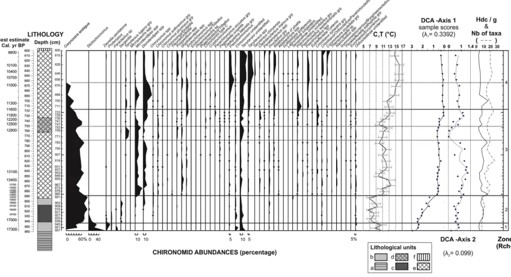
Sediment from 993 to 958 cm contained no chironomid head cap-sules. This may be explained by the climatic and environmental condi-tions that prevailed during the glacial period, which may have been too harsh for the occurrence of chironomids. Altogether 54 taxa were identified from the 41 levels sampled from 957 to 600 cm. A mean num-ber of 106.5 head capsules per sample were counted (nmin = 47 cap-sules at 945 cm, nmax = 243 at 700 cm), totaling 4369 head capcap-sules. The core sequence analysed was partitioned (following the “broken-stick” model) into four chironomid assemblage zones: RCh1 to RCh4 (Fig. 4).
After removal of rare taxa, DCA (Fig. 4and Supplementary Table 2) was performed on the 33 taxa in 41 samples totalling 4148 head cap-sules (95% of the whole dataset). DCA axes 1 and 2 have, respectively, eigenvalues of 0.34 and 0.09. The DCA-axis 1 gradient length is about 3 standard deviation (SD) units. Thefirst DCA axis is associated with both temperature and lake-level gradients related to both climate warming and the natural infilling of the lake as suggested by a fauna typical of the cold profundal zone of oligotrophic to mesotrophic lakes such as Stictochironomus (Wiederholm, 1983; Lotter et al., 1997; Brooks et al., 2007), Protanypus (Walker and MacDonald, 1995), Sergentia coracina (Brodin, 1986; Brooks et al., 2007), and Paracladius (Brooks et al., 2007) contrasting with a more littoral fauna of mesotro-phic to eutromesotro-phic warmer lakes with Parakiefferiella bathophila group
(Hofmann, 1984), Parachironomus arcuatus group (Buskens, 1987; Brodersen et al., 2001), Chironomus spp. (Brooks et al., 2007), Endochironomus spp. (Cranston, 2010), and Corynoneura scutellata group (Moller Pillot and Buskens, 1990). The second DCA axis is difficult to interpret because of the regrouping of both oligotrophic lacustrine taxa such as Tanytarsus lugens group (Brundin, 1956; Brodin, 1986) and Pagastiella orophila (Brooks et al., 2007) with the eutrophic lacus-trine taxon Polypedilum spp. (Brooks et al., 2007). This assemblage is op-posed to rheophilous taxa such as Eukiefferiella/Tvetenia (Wiederholm, 1983; Brooks et al., 2007) and other taxa associated with macrophytes such as Paratanytarsus spp. (Buskens, 1987; Brodersen et al., 2001), Corynoneura scutellata group (Kesler, 1981), and Cricotopus sylvestris group (Brodersen et al., 2001).
4.2.1. Zone RCh1: samples 957 to 945 cm (17,315 to 17,145 cal yr BP, best estimate)
Chironomid assemblages from RCh1 are characterized by the domi-nance of Stictochironomus and high percentages of Stempellinella/ Zavrelia, Paracladius, Protanypus, and Corynocera ambigua. The Stempellinella/Zavrelia group covers a wide range of ecological condi-tions from oligotrophic to eutrophic lakes and streams (Brooks et al., 2007; Wiederholm, 1983). Stictochironomus inhabits deep soft sediment or littoral sand of oligotrophic to mesotrophic lakes (Wiederholm, 1983).Korhola et al. (2002)consider it as cold stenothermous since this taxon preferentially colonizes arctic habitats (Danks, 1981). In NW Europe (Norway and Spitzbergen), Stictochironomus reaches a maximum abundance in lakes with Tjul air temperatures ranging from 8 to 14 °C (Brooks and Birks, 2000). In the Swiss Alps it occurs in lakes up to an elevation of 1500 m (Lotter et al., 1997), with Tjul air temper-atures ranging from 7.9 °C to 11.7 °C.
Quinlan and Smol (2001)consider the genus Paracladius to be indic-ative of highly oxygenated water. This genus can be considered as cold stenothermous, since it occurs in Swiss alpine lakes up to 1500 m (Lotter et al., 1997) in which Tjul air temperatures range from 7.6 °C to 10.7 °C.
Protanypus is also an indicator of highly oxygenated water (Quinlan and Smol, 2001) and colonizes cold (Olander et al., 1999) and oligotro-phic lakes (Wiederholm, 1983), preferring deep zones (Brooks and Birks, 2000). At present, this genus has its maximum occurrence at a July temperature ranging from 6 to 10 °C in Swiss lakes (Heiri and Millet, 2005).
Fig. 4. Summary diagram showing selected chironomid taxa encountered in Les Roustières sediments (%). The diagram zonation was determined using optimal sum of square partitioning (Birks and Gordon, 1985) using the software ZONE (Lotter and Juggins, 1991). The number of significant zones was determined by the “broken-stick” model using the BSTICK software (Birks and Line, unpublished). The statistically significant zones are delimited by solid lines. The dotted lines delimit the non-significant zone established by a constrained sum-of-squares cluster analysis (CONISS:Grimm, 1987). The names of lithological units (a–f) are given inFig. 3.
Corynocera ambigua has a wide modern geographical distribution ranging from northern to central Europe but is presently absent in France. The cold stenothermous character of C. ambigua has been questioned byBrodersen and Lindegaard (1999)who have shown mass occurrences of this species in warm water in Danish lakes (around 20 °C). These authors show that C. ambigua expansion is facilitated in clear waters, rich in benthic diatoms and with abundant aquatic vegeta-tion (such as charophytes). C. ambigua is broadly distributed along an elevational gradient in the subarctic region of northern Sweden (Larocque et al., 2001). In their dataset, the Tjul optimum of this taxon is 10.4 °C, which is relatively low for French latitudes.Larocque and Hall (2004)argue that there is no simple relationship between temper-ature, depth, and the occurrence of C. ambigua. This seems to be con-firmed byBarley et al. (2006), who show that the distribution and abundance of C. ambigua is not correlated with temperature but it is often abundant in shallow lakes in a north-west North American dataset where C. ambigua preferentially occurs in shallow lakesb4 m deep.
In summary, the chironomid fauna from zone RCh1 is characteristic of an oligotrophic lake with highly oxygenated waters in cold climatic conditions. The radiocarbon dates suggest this is towards the end of the Oldest Dryas. The rapid diminution of profundal taxa such as Stictochironomus and Protanypus suggests that water depth decreased throughout the zone, which probably facilitated the occurrence of C. ambigua.
4.2.2. Zone RCh2: samples 939 to 891 cm (17,040 to 15,210 cal yr BP, best estimate)
This zone is marked by the maximum abundance of C. ambigua (up to 90%), a decrease and almost disappearance of profundal taxa, such as Stictochironomus and Protanypus, and the appearance of littoral taxa, such as Microtendipes and Dicrotendipes, in the upper part of the zone. These taxa are also often associated with dense aquatic vegetation in shallow lakes or with warm summer temperatures (Hofmann, 1984; Brooks, 2006).
RCh2 is also marked by the appearance of Sergentia, a genus typical of arctic and alpine lakes with mesotrophic to oligotrophic waters (Lotter et al., 1997; Larocque et al., 2001).Heiri (2004)has shown that Sergentia tends to occur at higher abundances in the deepest part of shallow Norwegian lakes. This is also the case in north-west North America (Barley et al., 2006) where Sergentia preferentially occurs in lakes deeper than 4 m. The top of the zone is marked by thefirst occur-rence of thermophilic and mesotrophic to eutrophic taxa such as Chironomus and Dicrotendipes (Brodin, 1986), suggesting that the cli-mate was still cool but was starting to become warmer and that the lake was more nutrient-rich.
4.2.3. Zone RCh3: samples 885 to 723 cm (14,825 to 11,745 cal yr BP, best estimate)
This zone is marked by higher taxonomic richness than in the two previous ones. This indicates the habitat diversification that took place during the late-glacial interstadial climatic improvement. Hence, some thermophilic and mesotrophic to eutrophic taxa such as Glyptotendipes, Endochironomus (Larocque et al., 2001) and the Cladotanytarsus mancus group (Brooks et al., 2007) appear. Abundant taxa such as Microtendipes, Dicrotendipes, Glyptotendipes, and Ablabesmyia (e.g.,Brooks et al., 2007) are indicators of well-developed macrophytic vegetation around the lit-toral margins and suggest the prevalence of shallow-water conditions.
Several assemblagefluctuations are recorded in zone RCh3. The onset of the zone is characterized by occurrences of rheophilic genera such as Eukiefferiella/Tvetenia (Gandouin et al., 2006) which could be ex-plained by increased runoff from streams. This may be associated with the melting of snow patches in the area in response to regional climate warming. The 771 and 753 cm (12,960 and 12,695 cal yr BP, best esti-mate) levels are mainly characterized by a decrease in C. ambigua per-centages and high values of Tanytarsus lugens group. This last taxon usually occurs in the deep part of oligotrophic lakes or in the littoral
zone of cold subalpine and subarctic lakes (Brodin, 1986). This faunal change may be related to a rise in lake level and/or a climate cooling. The end of RCh3, from 735 to 723 cm (12,115 to 11,745 cal yr BP, best es-timate) is marked by a large decrease in C. ambigua and Microtendipes and a rise in several thermophilic taxa such as Endochironomus (Larocque and Finsinger, 2008), Dicrotendipes and Cladotanytarsus mancus group (Brooks et al., 2007), that are likely related to climate warming, probably the onset of the Holocene. Moreover, the continuous percentages of Ablabesmyia cf. phatta, a taxon associated with acidic conditions (Berezina, 2001) and peat-bog environments, may mark a reduction in the open-water surface of the site by telmatic peat develop-ment. Acidic conditions are also favourable to species of Psectrocladius (Brooks, 1996), Cladotanytarsus mancus group (Brooks et al., 2007), and Parachironomus arcuatus (Mousavi, 2002), which also increase from this point in the sequence.
4.2.4. Zone RCh4: samples 711 to 600 cm (11,435 to 9785 cal yr BP, best estimate)
Zone RCh4 is marked by the progressive disappearance of C. ambigua coupled with the rise in abundances of several taxa of Orthocladiinae (such as Psectrociadius genus, Corynoneura scutellata and Cricotopus/ Orthocladius/Paratrichocladius groups) and Chironomini (such as Glyptotendipes and Polypodium) which are linked to dense macrophytic vegetation (Brodersen et al., 2001; Brooks et al., 2007). RCh4 is also characterized by increasing percentages of thermophilic taxa such as Dicrotendipes, Pseudochironomus, and Chironomus. In thefirst part of RCh4, from 711 to 670 cm, littoral taxa such as Dicrotendipes, Endochironomus, and Microtendipes reach their maximum abundance, which could be related to abundant macrophyte growth in shallow wa-ters. In the terminal part of RCh4, from 658 to 600 cm, C. ambigua completely disappears and thermophilic taxa reach maximum abun-dance, which may indicate that the highest temperatures were reached. The rise in percentages of both Cricotopus/Orthocladius/Paratrichocladius and Corynoneura scutellata groups may be related to macrophyte devel-opment as the C. scutellata group is often associated with semi-submerged vegetation (Brooks, 2000) such as Typha, where the larvae are grazers on periphyton communities (Kesler, 1981).
4.2.5. Chironomid temperature reconstruction
TheTelford and Birks (2011)test indicates that the temperature re-construction from Les Roustières is statistically significant (p b 0.05) and suggests that temperature is the major driver of change in the chirono-mid assemblages. Two thirds of subfossil samples have a‘close’ ana-logue in the modern calibration data set (Fig. 5), but there are samples that have no close analogue in RCh-1 and Rch-4 chironomid zones. Nev-ertheless, the goodness-of-fit statistics revealed that only 22% of the samples have a‘poor’ fit in Rch-4. In the late-glacial, 22% of the samples have a‘poor’ fit and 34% have a ‘very poor’ fit with temperature. All the Younger Dryas samples have a‘good’ fit while it is the contrary for the Oldest Dryas. These lack-of-fit measures indicate that the fossil chiron-omid assemblages in those samples may be responding to changes in an environmental variable other than temperature. Hence the tempera-ture reconstructions from those samples, especially in the Older Dryas where goodness-of-fit values are particularly extreme, may be less reli-able and should be considered as tentative and interpreted with caution.
The reconstruction (Fig. 5) reveals several thermalfluctuations. The initial climate warming occurred around 15,000 cal yr BP when Tjul rose from 7 °C to 11 °C. A maximum of about 13.5 °C was reached around 13,800 cal yr BP. A second thermal optimum of 16 °C occurred after 10,800 cal yr BP in the earliest part of the Holocene. The late-glacial in-terstadial seems to be marked by decreases (−3 °C/−2 °C: from 13/12 to 10/9 °C) in summer temperature around 13,200 cal yr BP and 12,900 cal yr BP. A second climate minimum was reached when chironomid-inferred temperatures reached about 10 °C around 12,600 cal yr BP, in the Younger Dryas period. The end of the Younger
Dryas seems to have been warmer with summer temperatures of about 13 °C, just before the early-Holocene climate improvement.
4.3. Diatom analysis
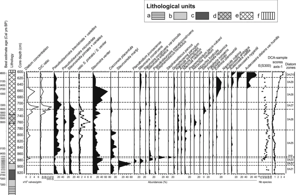
Sediment below 921 cm contained too few diatoms for counting. The core section analysed for diatoms, between 921 and 601 cm (Fig. 6), was partitioned into 10 diatom assemblages zones (RDaz1–10). The diatom flora of Les Roustières is composed of 149 species. For the statistical anal-yses, the original dataset was reduced to 65 samples and 132 species (species occurring inb2 samples at b0.2% were excluded). DCA axis 1 has a compositional turnover gradient length of 3.47 SD units and rep-resents 20.9% of the variation in the diatom data. This gradient is most likely primarily related to the dissolved organic carbon (DOC) content, with minimal values during RDaz6 and a maximum in the upper part of the sequence in RDaz10. RDaz6 is dominated by small species of Fragilariaceae that are generally associated with low DOC while RDaz10 is dominated by Aulacoseira spp. that generally prefer humic waters with high DOC concentrations (Ginn et al., 2007). This general distribution can be observed in the few datasets developed in northern Europe (Stevenson et al., 1991) and northern America (Fallu and Pienitz, 1999; Enache and Prairie, 2002) in which DOC is found to repre-sent a strong gradient. Although the actual values of the DOC optima and tolerance can be quite different between the datasets, as these de-pend on the range of the gradient, the Aulacoseira species appear to have consistently higher DOC optima than small-celled Nitzschia and Fragilariaceae species of the genera Staurosirella, Staurosira, and Pseudostaurosira. Staurosira construens var. binodis with a relatively
high DOC optimum and a high score on DCA axis-1 represents one ex-ception (Supplementary Table 1). Similarly in northern Sweden,
Korsman and Birks (1996) find that Aulacoseira species (e.g. A. ambigua, A. valida, A. nygaardii) are more abundant in highly coloured lakes (i.e. with high DOC content) than in clear-water lakes in which small Fragilariaceae such as Staurosirella lapponica and Pseudostaurosira pseudoconstruens are more abundant. In the Austrian Alps, Pseudostaurosira microstriata and Pseudostaurosira pseudoconstruens are found to characterize very low DOC lakes, with their optima around 0.5 mg L−1(Schmidt et al., 2004). In addition to DOC, DCA axis-1 may also represent a pH gradient as several acidophilous Eunotia spp. have a high DCA axis-1 score. The two variables DOC and pH, have been found to co-vary as the weak acids in DOC contribute to lowering the pH (Kingston and Birks, 1990,) although there is a complex relationship as chromophoric DOC can be degraded in strongly acidic lakes (Ginn et al., 2007). This explains why pH and DOC have also been found to be unrelated in various datasets (Dixit et al., 1993; Korsman and Birks, 1996). Nevertheless, changes in lake-water DOC are known to influence diatom distributions strongly as they affect water transparency, the un-derwater availability of light for photosynthesis via attenuation of pho-tosynthetically active radiation, the thermal and mixing regimes of the surface layer, and chemical interactions controlling the bioavailability of nutrients and trace metals (Cameron et al., 1999; Fallu et al., 2002). 4.3.1. Zone RDaz1: samples 921 to 901 cm (ca 16,580 to15,765 cal yr BP, best estimate)
Assemblages in RDaz1 are relatively rich with E(S300) up to 48 and
are dominated by small Fragilariaceae such as Staurosira venter,
Fig. 5. From left to right, chironomid-inferred temperature estimates (C-IT) with sample specific error bars; goodness-of-fit of the fossil assemblages to temperature, vertical dotted line indicates the 90th and 95th percentiles of squared residual distances of modern samples to thefirst axis in a CCA, samples to the right of the line have a poor or very poor fit-to-temperature respectively; nearest modern analogue analysis, vertical dotted line indicates the 2nd and 5th percentiles of squared chord distances of the fossil sample to samples in the modern calibration dataset, samples to right of line have no close and no good modern analogue respectively. The shaded areas correspond to samples that should be considered as tentative and interpreted with caution. OD: Oldest Dryas; LGI: late-glacial interstadial; YD: Younger Dryas; EH: early Holocene.
Fig. 6. Summary diagram showing selected diatom taxa encountered in Les Roustières sediments. The diagram zonation was determined using optimal sum of square partitioning (Birks and Gordon, 1985) using the software ZONE (Lotter and Juggins, 1991). The number of significant zones was determined by the “broken-stick” model using the BSTICK software (Birks and Line, unpublished). The names of lithological units (a–f) are given inFig. 3.
Pseudostaurosira brevistriata, Pseudostaurosira microstriata, and Staurosirella pinnata and its varieties. The average diatom concentration in this zone is fairly low (b1 × 106valves mg−1). Chrysophyte cysts are
abundant and the D/C ratio varies from 2.4 to 6.5. Small Fragilariaceae are typically very abundant in pioneer diatom communities that domi-nate ponds and lakes in arctic (Laing and Smol, 2000; Finkelstein and Gajewski, 2008) and alpine regions (Lotter and Bigler, 2000) with ex-tensive ice-cover. It is also interesting to note that in sediments formed at the time of deglaciation, fossil assemblages dominated by small Fragilariaceae are commonly reported in sediments deposited just after the retreat of the ice (Haworth, 1976). The small Fragilariaceae are primarily epipelic forms (Hickman, 1975). However, the epiphytic species Cocconeis placentula is also abundant (8 to 18%) in RDaz1 and suggests that aquatic macrophytes or mosses may have already been present in the lake.
4.3.2. Zone RDaz2: sample 890 (15,150 cal yr BP, best estimate)
This zone includes only one sub-sterile sample. Despite this, we de-cided to maintain this zone as its assemblage is clearly different from those in the samples above and below. Richness is very low (10 species). This is the only sample in which chrysophyte cysts are more abundant than diatoms (D/C ratio = 0.3). Staurosirella martyi is largely dominant (60%) in this sample. Staurosirella pinnata and Staurosira venter are sub-dominant species. S. martyi (= Martyana martyi = Fragilaria leptostauron var. martyi) has been reported as epipsammic, i.e. living on sand grains (Round et al., 1990). Mass occurrences of S. martyi have been often reported in calcium-rich sediments and in calcareous gyttja (Witkowski et al., 1995). This zone may therefore correspond to an episode of increased mineral influx to the lake, presumably as a result of erosion of less stable soils.
4.3.3. Zone RDaz3: samples 881 to 873 cm (14,560 to 14,050 cal yr BP, best estimate)
Compared with the previous zone, the average diatom concentration increases markedly to 0.7 × 10⁶valves mg−1. The D/C ratio increases sharply up to 23. Assemblages are still dominated by small Fragilariaceae but become more diverse than in RDaz2 with Staurosira venter, S. elliptica, S. construens, S. construens var. binodis, Pseudostaurosira pseudoconstruens, P. brevistriata, P. microstriata, and Staurosirella pinnata and its varieties. Planothidium joursacence, general-ly described in the literature as a Nordic alpine species, is abundant (11%). E(S300) increases through the zone, up to 30. The diatoms of
this zone still indicate a pioneer assemblage.
4.3.4. Zone RDaz4: samples 870 to 869 cm (13,885 to 13,835 cal yr BP, best estimate)
This zone is characterized by a high abundance of the planktonic species Stephanodiscus minutulus (30%) and S. parvus (15%) combined with a sharp decrease in small Fragilariaceae and an increase of epiphyt-ic diatoms such as Cocconeis placentula and Gomphonema parvulum. Di-atom concentration declines slightly (0.4 × 10⁶valves mg−1). Richness
increases further, with E(S300) up to 38. The two small planktonic
Stephanodiscus species are typically associated with meso- to eutrophic conditions (Padisàk et al., 2009; Berthon et al., 2013). This zone suggests a deeper and more productive lake in which a truly planktonic diatom community could develop along with macrophytes. This suggests a large increase in the duration of the growing season.
4.3.5. Zone RDaz5: samples 865 to 788 cm (13,645 to 13,060 cal yr BP, best estimate)
Stephanodiscus species sharply decline and small Fragilariaceae again dominate the assemblages with Pseudostaurosira brevistriata and Staurosira venter as the most abundant species. Aulacoseira valida is common in the assemblages. Diatom concentration, on average, in-creases slightly. Richness inin-creases markedly, especially towards the top of the zone with a peak value for E(S300) of 53. This zone suggests
a decrease in water depth such that planktonic diatoms could not devel-op large pdevel-opulations.
4.3.6. Zone RDaz6: samples 778 to 719 cm (13,015 to 11,640 cal yr BP, best estimate)
Percentages of small Fragilariaceae increase further with, in particu-lar, high abundances of Staurosirella pinnata, P. microstriata, and P. pseudoconstruens. Staurosirella lapponica is only abundant at the top of the zone. Staurosira venter decreases markedly in the middle of the zone. Diatom concentration and the D/C ratio both increase sharply to-wards the top of the zone. The epipelic Nitzschia bacillum and N. fonticola are common. These small-celled Nitzschia are particularly good indica-tors of low DOC concentrations (Fallu and Pienitz, 1999; Fallu et al., 2002). Percentages of C. placentula decrease sharply, indicating a much reduced presence of macrophytes. Diatom richness declines throughout the zone, down to E(S300) at 30. Interestingly,Birks et al.
(2012)report from northern Norway during the same time interval a diatom assemblage totally dominated by S. pinnata that they interpret as indicating very cold and turbid waters. Studies on the modern distri-bution of these taxa in the Canadian Arctic (Joynt and Wolfe, 2001; Bouchard et al., 2004) and northern Sweden (Rosén et al., 2000) show that the various species of Fragilariaceae have different optima for sum-mer water temperature with Staurosirella taxa living in colder water than Staurosira taxa. In circumpolar lakes in northern Russia,Laing and Smol (2000)find Staurosirella pinnata to be more abundant in the tundra zone, while Staurosira venter has higher abundances in lakes lo-cated at lower latitude in the boreal forest zone, and characterized by warmer surface water temperatures. Similar shifts in dominance be-tween species of small Fragilariaceae have been observed in Canadian sequences, in whichPodritske and Gajewski (2007)observed a clear in-verse relationship between Staurosira and Staurosirella. Similarly,
Finkelstein and Gajewski (2008)used the ratio of Staurosirella pinnata to Staurosira venter as an indicator for warm and cold phases in their re-cord from the Canadian Arctic. The same ratio applied to Les Roustières diatom sequence clearly distinguishes RDaz6 as the coldest phase in our record. In support of this interpretation, P. microstriata has the low-est optima for July temperature and the highlow-est optima for the length of ice-cover in a modern dataset from the Austrian Alps (Schmidt et al., 2004).
4.3.7. Zone RDaz7: samples 714 to 702 cm (11,510 to 11,240 cal yr BP, best estimate)
Assemblages are still dominated by small Fragilariaceae, although the percentages of the main species are different from those in the pre-vious zone with lower Staurosirella pinnata and much higher P. brevistriata. Diatom concentration reaches its highest value for the whole profile (6 × 10⁶valves mg−1) and chrysophyte cysts are very
few. Richness remains at a relatively low level with E(S300) between
31 and 38. Epiphytic species such as Gomphonema parvulum and Fragilaria rumpens are common. The sharp decline in the S. pinnata/ S. venter ratio and the apparent increase in aquatic vegetation and in productivity suggest warmer conditions than in the previous zone. 4.3.8. Zone RDaz8: samples 689 to 652 cm (11,100 to 10,660 cal yr BP, best estimate)
Staurosira venter largely dominates the assemblage while P. brevistriata decreases. Towards the top of the zone motile, epipelic species such as Eolimna utermoehlii and the large-celled Navicula vulpina increase markedly while epiphytic species decrease. Diatom concentra-tion decreases while chrysophyte cysts become more abundant. Diatom richness declines markedly towards the top of the zone with E(S300)
down to 18. The increase in the relative abundance of Eunotia minor, a species regularly found on mosses (Alles et al., 1991; Bertrand et al., 2004; Pavlov and Levkov, 2013) may indicate the development of a peat bog.
4.3.9. Zone RDaz9: samples 644 to 620 cm (10,450 to 9925 cal yr BP, best estimate)
Assemblages are dominated by the planktonic Aulacoseira valida, A. nygaardii, and A. distans var. humilis while the abundance of Eolimna utermoehlii (=Navicula subrotundata) increases further. Diatom con-centration decreases further (0.8 × 10⁶valves mg−1) and richness
in-creases with E(S300) above 30. The Aulacoseira spp. indicate fairly high
concentrations of DOC (Supplementary Table 1; Stevenson et al., 1991; Fallu and Pienitz, 1999; Enache and Prairie, 2002). Low levels of light, generally associated with high DOC, may have been favourable to large populations of E. utermoehlii that was reported as a characteris-tic benthic motile diatom of deep-water assemblages (Kingston et al., 1983). This species is also found to be associated with warm and nitrogen-rich waters (Kocev et al., 2010).
4.3.10. Zone RDaz10: samples 613 to 601 cm (9845 to 9785 cal yr BP, best estimate)
In this zone the diatom concentration decreases significantly from 0.3 to 0.06 × 10⁶ valves mg−1. Samples above 601 cm are sterile. The assem-blages are characterized by dominant Aulacoseira distans var. humilis and by subdominant A. nygaardii (60–70% together). The last sample is almost entirely composed of cingulum of Aulacoseira spp. with no entire valves. Diatom richness decreases with E(S300) below 20. Eolimna utermoehlii
de-clines sharply and epiphytic diatoms almost disappear from the assem-blages, which suggest the decline of macrophytes and may relate to low light conditions unfavourable for benthic diatoms. The relative domi-nance of planktonic Aulacoseira spp. and low diatom concentration sug-gest dystrophic conditions, characterized by low phytoplankton production and high organic content (Wetzel, 2001).
5. Discussion
5.1. Past lacustrine environmental reconstruction based on multiproxy evi-dence (comparison between diatom, chironomid, pollen, and lithological results)
5.1.1. Oldest Dryas period (RCh1–2, RDaz1–2, grey clayey sediment) The base of the sequence at Les Roustières, between 17,700 to 16,600 cal yr BP is marked by the absence of diatoms, whereas chirono-mids are well represented. This may be due to high water turbidity or persistent ice-cover (due to extreme climate conditions), which may have decreased the amount of light available for photosynthetic activi-ties, and thus strongly reduced lacustrine primary productivity. Alterna-tively, relatively high pH and a low silica concentration may have caused poor preservation of diatom remains. The contemporaneous chi-ronomid assemblages are composed mainly of profundal, cold, oligotro-phic taxa. This is also supported by the sedimentation of clay. Summer temperatures during this period were lower than or equal to 10 °C (Fig. 7) which is not favourable for high lacustrine productivity. The sub-sterile RDaz2 zone is also contemporaneous with a minimal sum-mer temperature of around 7 °C. At the end of the Oldest Dryas, between ca 16,400 and 15,000 cal yr BP, chironomids and diatoms together point to a cold oligotrophic (to mesotrophic) lake with shallow waters, with the probable presence of aquatic macrophytes on littoral margins. How-ever, very few pollen grains of Potamogeton and Myriophyllum were re-corded in the pollen analysis (Fig. 3).
5.1.2. Late-glacial interstadial (RCh3a, RDaz3–5 and gyttja sediment) Both diatom and chironomid evidence suggest that the onset of the late-glacial interstadial (LGI) is marked by taxonomic diversification,
Fig. 7. Comparison between the pollen stratigraphy, lithology, chironomid-inferred temperature reconstruction (CI-T), and the diatom ratio Staurosirella pinnata/Staurosira venter. The names of lithological units (a–f) are given inFig. 3.
moderate water eutrophication, and growth in aquatic vegetation, probably in response to climatic improvement. This is confirmed by an increase in Potamogeton and Myriophyllum abundance (Fig. 3). Howev-er, the abundances of both cold-adapted diatoms and chironomids over the LGI seem to indicate relatively moderate but unstable summer tem-peratures (never exceeding 14 °C), as shown by the fluctuating chironomid-inferred temperature curve and the S. pinnata/S. venter ratio (Fig. 7). A probable cold event is indicated by pollen data from Les Roustières that show a sharp decrease in the AP/NAP ratio around 13,000 cal yr BP (Fig. 7), related to rises in Artemisia and Poaceae per-centages. This vegetation dynamic is contemporaneous with a slight rise in the S. pinnata/S. venter ratio only. This cold event, may be related to the GI-1b cold event recorded in the NGRIP ice-core, which is also named the Intra-Allerød Cold Period in terrestrial records from the North Atlantic region or the Gerzensee oscillation in central European lakes.
5.1.3. Younger Dryas (RCh3b-c, RDaz6 and clay-gyttja sediment) The Younger Dryas event is well marked in both the diatom and chi-ronomid assemblages, as shown by the decrease or absence of ther-mophilous chironomid taxa and the simultaneous rise in the S. pinnata/S. venter ratio. This climatic deterioration is also indicated in the pollen results with a fall in the AP/NAP ratio that is associated with decreasing percentages of Pinus and increasing percentages of the steppic taxa Artemisia and Chenopodiaceae (Fig. 3).
In addition, the YD event induced a change in the hydrological re-gime of the basin with more oligotrophic water and a probable decrease in the input of allochthonous organic matter (as suggested by the in-crease in abundances of the diatoms Nitzschia fonticola and N. bacillum that indicate low DOC concentrations). This may have been a conse-quence of the freezing of small rivulets feeding the lake during the major part of the year. Lastly, a decrease in macrophytes is indicated by the fall in macrophyte associated diatoms (e.g. Cocconeis placentula) and chironomids such as Dicrotendipes in RCh-3b sub-zone, which is consistent with slightly lower abundances of Potamogeton and Myriophyllum (Fig. 3) than during the LGI.
5.1.4. Early Holocene (RCh4, RDaz7–10, organic gyttja and peat) Both macrophytic chironomid fauna (such as Glyptotendipes, Dicrotendipes and Polypedilum) and epiphytic diatom species (such as Gomphonema parvulum and Fragilaria rumpens) show a shallowing of the lake with climatic improvement that occurred at the beginning of the Holocene. Maximal abundances of Potamogeton and Myriophyllum (Fig. 3) indicate dense hydrophytic vegetation into the persistent open waters close to the extended peat-bog. Palustrine environment is also indicated by the increasing abundances of the acidophilic chironomid taxa such as Ablabesmyia cf. phatta and Psectrocladius sordidellus (Fig. 4) and diatoms such as Aulacoseira spp. (Fig. 6). Les Roustières basin was probably largelyfilled-in at that time.
5.2. Reliability of the chironomid-based temperature reconstruction Several samples, especially those in the Older Dryas, have a poor- fit-to-temperature. Moreover, DCA sample scores (Fig. 4) show that while the axis 2 scores reflect the major trends in the C-IT reconstruction, the axis 1 scores, which reflect the major environmental driver of the chi-ronomid assemblage composition, show a different pattern. These re-sults suggest that variables other than temperature may have been influencing the response of the chironomid assemblages at this time. Other variables known to influence chironomid distribution and abun-dance include water depth, pH oxygen conditions, and trophic level (Brooks et al., 2016; Juggins, 2013). Hence, this raises the question about the major forcing factor for the chironomid fauna at Les Roustières. The chironomid fauna is dominated from the Older Dryas to the end of the Younger Dryas by C. ambigua, which has a strong influence on the temperature reconstruction, as indicated by the striking inverse
correlation between C. ambigua percentage abundance, the tempera-ture curve and the DCA axis 1 scores. C. ambigua has an ambiguous re-sponse to temperature (Brodersen and Lindegaard, 1999) and it may also be responding to the natural infilling of the site and fluctuations in lake-level. However, it is clear that the CI-T is correlated with the mainfloristic and diatom changes. The temperature (CI-T) decreases are contemporaneous with both landscape openings and rise in the S. pinnata / S. venter ratio, which argues for cold climate conditions (Fig. 7). These evidences makes us confident that temperatures were relatively low during the Older Dryas part of the sequence.
5.3. Regional comparison
Thefirst attempt at a climate reconstruction at the Taphanel site was done byPonel and Coope (1990), based on fossil Coleoptera assem-blages using the Mutual Climatic Range method (Atkinson et al., 1987). The Taphanel record is located within 80–100 km of Les Roustières peat bog and at an elevation of almost 1000 m asl. With the exception of the difference in elevation between the two sites, the two records are located in a similar climate context that allows direct com-parison (Table 2) between chironomid-inferred July temperature and TMAX(mean temperature of the warmest month). The
chironomid-inferred temperature reconstruction has a better sampling resolution and a lower temperature range but is in good agreement with the MCR data, especially when temperature ranges for coleopteran data are narrow.
According toPonel and Coope (1990), the late Würm and Oldest Dryas climates were of arctic severity and considerably more continen-tal than at present. MCR coleopteran reconstructions have shown that summer temperatures ranged from 7 to 13 °C. Chironomid data suggest that the mean July air temperatures ranged probably from 6 to 10 °C.
The Ponel and Coope (1990) reconstructions show a climatic warming at about 13,000 uncalibrated yr BP (about 15,000 cal yr BP) followed by the Bølling temperate episode. This climate improvement is confirmed by the rise in chironomid-inferred temperatures just after 15,200 cal yr BP (cf., best estimate age). However, based on chiron-omid data, this warming is moderate compared to the maximum values suggested by MCR. This cooler climate is confirmed by the abundance of cold diatom species at Les Roustières throughout the LGI.
Ponel and Coope (1990)identified a marked deterioration in sum-mer warmth for a short period between the Bølling and Allerød, which is perhaps the Older Dryas period. Nevertheless, we note that this interpretation is not supported by an increase in cold beetle species but only by the MCR inference being better constrained for this particu-lar sample. In addition, the absence of both absolute14C dating and an age-depth model for La Taphanel record and the low sample resolution of the coleopteran analysis, make it impossible to establish a more accu-rate chronological correlation with Les Roustières for this interval.
As suggested by the Coleoptera at La Taphanel, the Allerød period was decidedly cooler than the Bølling. The chironomid data from Les Roustières do not confirm this hypothesis, with maximum temperatures reached between 13,800 and 13,400 cal yr BP, during the Allerød. Nev-ertheless, midges suggest that the Allerød period was marked by cli-mate instability (confirmed by several proxies cf.,Fig. 7) occurring between 13,300 and 12,900 cal yr BP. It is also possible that the Coleop-tera analysis failed to detect such a short-lasting event due to its coarse temporal resolution, as the large volume of sediment required for this type of analysis results in very thick samples of low temporal resolution. This may lead to the pooling of cool and warm phases and thus to an under- or over-estimation of the coleopteran TMAXvalues.
At La Taphanel, the climate deterioration of the Younger Dryas is marked by a drop in summer temperatures with a probable return to conditions similar to the Oldest Dryas and a rise in continentality. The chironomid record from Les Roustières suggests that this cooling in sum-mer temperatures was somewhat limited, as Younger Dryas Tjul were 2–3 °C higher than those of the Oldest Dryas. This has already been
Table 2
Temperature comparisons between late-glacial European records. Numbers in brackets indicate temperature ranges (“+” warming; “−” cooling). *Corrected values have been calculated with elevational and latitudinal correcting factors, using the lapse rates of 0.6 °C per 100 m elevation and 0.6 °C per 1° latitude, which are often used for summer temperatures. These corrected values correspond to probable values that the reference site would have received if it was located at the same latitude and elevation as Les Roustières.
Location References Oldest Dryas Corrected
values*
Bølling Corrected
values*
Allerød Corrected
values*
Younger Dryas Corrected
values*
Early Holocene Corrected
values*
Les Roustières (1196 m) This study 6 to 10 °C – – 11 °C (+4 °C) – – 12 to 13 °C (+1 to 2 °C) – – ca 10° & 13 °C (−2 °C) – – 12 to 16 °C (+3 °C) – –
Lautrey (788 m) Peyron et al. (2005) 11 to 12 °C 10.3 11.3 15.5 to 16 °C (+5 °C) 14.8 15.3 15.5 to 18.4 °C (+2 to 3 °C) 14.8 17.7 13.6 to 13.9 °C (−3 to −4 °C; sec. part +0.3 °C) 12.9 13.2 13.9 to 15.5 °C (+1.5 to 3 °C) 13.2 14.8
Lautrey (788 m) Heiri and Millet (2005) 11 to 12 °C 10.3 11.3 14 to 16 °C (+3 to 3.5 °C) 13.3 15.3 15.8 16.7 14 to 15 °C (−2.5 to −3.5 °C) 13.3 14.3 16°5 15.8 –
Ech (710 m) Millet et al. (2012) 10 to 13 °C 6.7 9.7 16 to 17.5 °C (+6 °C) 12.7 14.2 ca. 16.5 °C (−1 °C) 16.5–17 °C
13.2 – 15 to 15.5 °C (−1.5 °C) 11.7 12.2 ca. 17 °C 15.7 –
La Taphanel (975 m) Ponel and Coope (1990) 7 to 13 °C 6.0 12.0 11 to 23 °C 10.0 22.0 11 to16°C 10.0 15.0 6 to 18 °C 5.0 17.0 10 to 23 °C 9.0 22.0
Gerzensee (603 m) Lotter et al. (2012) About 11 °C 9.3 – 12 to 14 °C (+2 to 3 °C) 10.3 12.3 14 to 16 ° C 12.3 14.3 – – – – – –
Egelsee (770 m) Larocque-Tobler et al. (2010)
ca. 11.4 °C 11 – ca. 17 °C (+3 to 4 °C) 16.6 ca. 15.5 °C 15.1 – ca. 13.9 °C (−1.5 °C) 13.5 Average of 15.3 °C (+3 °C) 14.9 –
Hinterburgsee (1515 m) Heiri et al. (2003) – – – – – – – – – 10.4 to 10.9 °C 14.2 14.7 11.9 to 12.8 °C 15.7 16.6
Maloja pass (1815 m) Ilyashuk et al. (2009) – – – – – – 10 to 11.7 °C 15.6 17.3 8.8 & 9.8 °C (−3.5 to −4 °C) 14.4 15.4 13.6 to 13.9 °C
(−3.5 to −4 °C)
19.2 19.5 Lago di Piccolo (365 m) Larocque and Finsinger
(2008)
ca.16 °C (only one sample)
14.3 ca. 19 °C (+3 °C) 17.3 ca. 17 °C 15.3 – ca. 16 °C (−1.5 °C) 14.3 ca. 18.5 °C (+2.5 °C) 16.8
L. di Lavarone (1(100 m) Heiri et al. (2007b) 10.5 to 10.8 °C 11.2 11.5 13.8 to 13.9 °C (+3 °C) 14.5 14.6 15.3 °C just before YD 16.0 – 11.7 to 14.5 °C (−2 °C) 12.4 15.2 15.8 to 16.4 °C (+2.5 °C) 16.5 17.1 Hijkermeer (14 m) Heiri et al. (2007a) – – – 14 to 16 °C imprecise14C 12.4 14.4 16 to 16.5 °C 14.4 14.9 13.5 to 14 °C (−2 to −3 °C) 11.9 12.4 15.5 to 16 °C (+2 to 3 °C) 13.9 14.4
Five sites (8 to 250 m) Lang et al. (2010) – – – 12 to 13 °C 12.5 13.5 – – – 8 to 10 °C (average of−4.5 °C) 8.5 10.5 15.5 to 16 °C (+5 °C) 16.0 16.5
Haweswater (8 m) Bedford et al. (2004) 7.4 to 10 °C 6.5 9.1 ca.13.4 °C (+3 to +4 °C) 12.5 – ca. 11.4 °C (−2 °C) 10.5 – 7.5 °C & 10 °C (− 6 °C) 6.6 9.1 13.8 °C (+4 to 5 °C) 12.9 – L. Nadourcan (70 m) Watson et al. (2010) 7.5° to 9 °C 7.6 9.1 ca. 13 °C (+5 °C) 13.1 – ca. 12 °C (−1 to −2 °C) 12.1 – 7.5 to 10 °C (−5 °C and +2.5 °C
over the YD)
7.6 10.1 Around 14 °C (+4 to 5 °C) 14.1 – Whitrig Bog (125 m) Brooks and Birks (2001) 6 °C (only one
sample)
– 6.8 10.5 to 12 °C (+5 to 6 °C) 11.3 12.8 ca.11 °C (−1° over the YD)
11.8 – 7.5 °C to 9 °C (−2.5 to −3.5 °C) 8.3 9.8 11.5 °C (+2.5 °C) 12.3 –
Location References GI-1d Corrected values* GI-1b Corrected values* PBO Corrected values*
Les Roustières This study 10 °C
(−1 °C) – –(−1 °C) – – –(−0.5 to −1 °C) – –
Lautrey (788 m) Peyron et al. (2005) ca. 15 °C
(−0.75 to −1 °C) 14.3 16.8 to 15 ° C (−2 °C) 14.3 16.1 17.5 to 14 °C (−3.5 °C) 13.3 16.8
Lautrey (788 m) Heiri and Millet (2005) – – –
(−1.5 to −2 °C) – – – – –
Ech (710 m) Millet et al. (2012) –
(−1.5 °C) – – – – – – –
La Taphanel (975 m) Ponel and Coope (1990) – – – – – – – –
Gerzensee (603 m) Lotter et al. (2012) –
(−0.5 to −1 °C) – – – – – – –
Egelsee (770 m) Larocque-Tobler et al. (2010) – – – – – − (−1 °C) – –
Hinterburgsee (1515 m) Heiri et al. (2003) – – – 10.4 to 11.1 °C
(−0.8 °C)
14.1 14.9
Maloja pass (1815 m) Ilyashuk et al. (2009) ca 9 °C
(−2.1 °C)
14.6 ca 6 °C
(−1.4 °C)
11.6 – – – –
Lago di Piccolo (365 m) Larocque and Finsinger (2008) – – – – – – – –
L. di Lavarone (1(100 m) Heiri et al. (2007b) – – – – – − (−0.5 °C) – –
Hijkermeer (14 m) Heiri et al. (2007a) –
(−1.5 °C) – –(−2.1 °C) – – – – –
Five sites (8 to 250 m) Lang et al. (2010) –
(−0.6 to −2.6 °C) – –(−0.8 to −1.6 °C) – – − (up to −1 °C) – –
Haweswater (8 m) Bedford et al. (2004) No date;
(−1 to −1.5 °C) – – – – − (−1 to −1.5 °C) – –
L. Nadourcan (70 m) Watson et al. (2010) ca.11 °C
(−2.5 °C)
11.1 ca. 12 °C
(−1 to −1.5 °C)
12.1 – – – –
Whitrig Bog (125 m) Brooks and Birks (2001) ca. 8 °C
(−1.5 to −2 °C)
8.8 About 9.5 °C
(inferior to−1 °C)