HAL Id: hal-02880225
https://hal.archives-ouvertes.fr/hal-02880225
Submitted on 2 Sep 2020
HAL is a multi-disciplinary open access
archive for the deposit and dissemination of
sci-entific research documents, whether they are
pub-lished or not. The documents may come from
teaching and research institutions in France or
abroad, or from public or private research centers.
L’archive ouverte pluridisciplinaire HAL, est
destinée au dépôt et à la diffusion de documents
scientifiques de niveau recherche, publiés ou non,
émanant des établissements d’enseignement et de
recherche français ou étrangers, des laboratoires
publics ou privés.
Experimental and numerical assessment of deterministic
nonlinear ocean waves prediction algorithms using
non-uniformly sampled wave gauges
Nicolas Desmars, Félicien Bonnefoy, Stéphan Grilli, Guillaume Ducrozet, Yves
Perignon, Charles-Antoine Guérin, Pierre Ferrant
To cite this version:
Nicolas Desmars, Félicien Bonnefoy, Stéphan Grilli, Guillaume Ducrozet, Yves Perignon, et al..
Ex-perimental and numerical assessment of deterministic nonlinear ocean waves prediction algorithms
using non-uniformly sampled wave gauges.
Ocean Engineering, Elsevier, 2020, 212, pp.107659.
Experimental and numerical assessment of deterministic nonlinear ocean
waves prediction algorithms using non-uniformly sampled wave gauges
N. Desmars
a,∗, F. Bonnefoy
a, S.T. Grilli
b, G. Ducrozet
a, Y. Perignon
a, C.-A. Guérin
c, P. Ferrant
aaÉcole Centrale de Nantes, LHEEA Res. Dept. (ECN and CNRS), 44321 Nantes, France bDepartment of Ocean Engineering, University of Rhode Island, Narragansett, RI 02882, USA
cUniversité de Toulon, Aix-Marseille Université, IRD, CNRS-INSU, Mediterranean Institute of Oceanography (MIO UM 110), 83957 La Garde, France
We assess the capability of fast wave models to deterministically predict nonlinear ocean surface waves from non-uniformly distributed data such as sampled from an optical ocean sensor. Linear and weakly nonlinear prediction algorithms are applied to long-crested irregular waves based on a set of laboratory experiments and corresponding numerical simulations. An array of wave gauges is used for data acquisition, representing the typical spatial sampling an optical sensor (e.g., LIDAR) would make at grazing incidence. Predictions of the weakly nonlinear Improved Choppy Wave Model are compared to those of the Linear Wave Theory with and without a nonlinear dispersion relationship correction. Wave models are first inverted based on gauge data which provides the initial model parameters, then propagated to issue a prediction. We find that the wave prediction accuracy converges with the amount of input data used in the inversion. When waves are propagated in the models, correctly modeling the nonlinear wave phase velocity provides the main improvement in accuracy, while including nonlinear wave shape effects only improves surface elevation representation in the spatio-temporal region where input data are acquired. Surface slope prediction accuracy, however, strongly depends on the appropriate nonlinear wave shape modeling.
1. Introduction
The availability of real-time phase-resolved wave fields is key for the optimization of a vast range of marine applications. The prediction and control of the wave-induced motion is crucially important to extend the operational envelope and optimal maneuvering of many surface vessels, such as to stabilize aircraft or helicopter carriers during takeoff/landing manoeuvres, ships during ship-to-ship transfer, or to perform installation and maintenance operations on marine structures. For ocean renewable energy harvesting systems, advance knowledge of incoming waves conditions the performances of control strategies. For instance, it is shown that the optimal control of wave energy converters relying on wave-to-wave predictions significantly improves their effi-ciency (Li et al.,2012). Also, the life-time of floating wind turbines could be increased by mitigating fatigue loads through appropriate control of the structure motions induced by wave loads (Ma et al.,
2018).
The deterministic prediction of ocean wave fields requires inverting a model describing the wave dynamics based on a set of observations, i.e., measurements that contain information about the wave geometry and kinematics (e.g.,Nouguier et al.,2014). Based on such an inversion
∗ Corresponding author.
E-mail address: [email protected](N. Desmars).
(i.e., nowcast), the properly parameterized wave model can then be used to propagate the wave field forward in time (i.e., forecast) to the area of interest. Note that the later can itself be in motion (e.g., a moving ship).
X-band radars, such as WaMoS II developed by OceanWaveS GmbH™ (Hilmer and Thornhill,2015), the prediction systems of Next Ocean™ (Naaijen et al.,2018), or FutureWaves™ (Kusters et al.,2016), have been used to generate large spatio-temporal data sets of wave elevations surrounding the structure upon which they are mounted. Such radars make use of the backscattered signal resulting from the Bragg resonance between the radar microwaves (∼3 cm wavelength) and short-wavelength capillary–gravity waves (∼1.5 cm wavelength) covering the ocean surface due to wind generation. Hydrodynamic and tilt modulations of such short ripples by longer gravity waves carrying them, that affect the backscattered signal, allow inverting for surface elevations by means of a modulation transfer function (MTF) (Nieto Borge et al.,2004), provided that a calibration is enabling a retrofit on this MTF in the measurement chain. This technology has been successfully implemented in commercial products (Hilmer and Thornhill,2015;Kusters et al.,2016;Naaijen et al.,2018).
Similar data sets can be obtained by the way of LIDAR (LIght Detection and Ranging) cameras (Belmont et al., 2007; Grilli et al.,
2011; Nouguier et al., 2014; Kabel et al., 2019), which operate in the visible light (e.g., green; 532 nm wavelength). Instead of using modulation properties of Bragg waves to estimate gravity waves char-acteristics, LIDAR cameras provide direct geo-referenced measurements of free surface elevations, computed based on laser beam travel times. One advantage of this technique, as compared to X-band radars, is the higher spatial resolution resulting from the smaller divergence of the laser beams compared to the microwave beams (Sviridov,1993), providing a more accurate phase resolved (instantaneous) measurement of the ocean surface.
When mounted on an ocean structure or surface vessel to remotely measure ocean surface elevations, both X-band radar and LIDAR cam-era have limitations resulting from the grazing incidence angles of the beams. First, it will cause wave shadowing effects, leading data sets ac-quired by these systems to exhibit spatial gaps behind illuminated wave fronts which have an area increasing with the distance from the sensor. Second, assuming a uniform distribution of beams over the sensor’s aperture angles, the density of the measurement points geometrically decreases with the distance from the sensor. In the case of X-band radars, shadowing effects are used to generate a shadowing mask that is implemented in the MTF used for wave inversion (Nieto Borge et al.,
2004). For LIDAR cameras, the lack of information in the shadowed area can be compensated for by using spatio-temporal data sets, i.e., at a slightly later time, shadowed areas without measurement points can become illuminated due to wave motion. This, however, also requires performing a spatio-temporal wave field inversion (Grilli et al.,2011;
Nouguier et al.,2014;Desmars et al.,2018). In addition to generating spatial gaps, shadowing effects cause laser beams to hit the ocean surface at unknown horizontal locations, leading the measurement points to be distributed over an a priori unknown unstructured grid. These properties, together with the non-periodicity of observations, prevent using standard signal-processing techniques based on Fourier decomposition in the wave inversion, unless a pre- or post-processing method is used (e.g., interpolation, end-matching, filtering).
Due to real-time constraints, i.e., sufficient computational effi-ciency, existing deterministic wave prediction systems have typically used models based on linear wave theory (LWT) (Hilmer and Thornhill,
2015;Kusters et al.,2016;Naaijen et al.,2018). However, this limits their applicability to sea states with a small characteristic steepness, and further assumes that: (i) bound waves (i.e., harmonic waves that do not obey the dispersion relation) can be neglected, and (ii) the space and time scales of observations and the prediction horizon do not allow time-dependent nonlinear wave-wave interactions (e.g., nonlin-ear phase shift) to significantly affect wave dynamics. Whenever these limitations are not met, the accurate prediction of ocean surface waves will require modeling weakly or fully nonlinear wave properties.
Weakly nonlinear models have been developed and used for wave simulation and prediction based on expanding Eulerian wave properties up to the second-order in wave steepness (e.g., Zhang et al., 1996,
1999), which for instance allows separating free- and bound-wave components in wave measurements. A model based on the Modified NonLinear Schrödinger (MNLS) equation, which simulates third-order wave properties such as phase speed, was used to predict bichromatic waves (Trulsen and Stansberg, 2001), then extended to both one-directional and one-directional irregular seas (Simanesew et al., 2017). The latter study showed that the MNLS equation is able to provide satisfactory predictions of long-crested irregular waves, but the lack of directional input data prevented properly estimating its predic-tion performance for short-crested waves with increasing direcpredic-tional spread. Higher-order wave models based on the High-Order Spectral (HOS) method were also applied for nonlinear prediction of ocean surfaces (e.g.,Wu,2004;Blondel et al.,2010;Qi et al.,2018a). Based on a pseudo-spectral approach, this method solves the nonlinear free
surface boundary conditions to an arbitrary order for a velocity po-tential, and allows to simulate the propagation of any wave fields over large space and time scales with a high accuracy. Predictions of long-crested irregular waves using both HOS, LWT and nonlinear Schrödinger approaches were recently compared (Klein et al., 2020), showing that the appropriate modeling of nonlinear dispersion effects plays a significant role from moderate to high wave steepness, with HOS being the most accurate prediction model. The main counterpoint of HOS is its initialization process that necessitates a high number of operations, exponentially increasing with its order of nonlinearity. Recent works have been carried out on improved assimilation methods for HOS to be adequate for real-time prediction (Köllisch et al.,2018;
Fujimoto and Waseda,2020).
In this study, we apply and experimentally validate a wave recon-struction and prediction algorithm based on the recently developed Improved Choppy Wave Model (ICWM) (Guérin et al.,2019), which extends with higher-order corrections the weakly nonlinear Lagrangian Choppy Wave Model (Nouguier et al.,2009), which was used in our earlier work on ocean wave reconstruction algorithms based on LIDAR camera data (Grilli et al.,2011;Nouguier et al.,2014).
The paper is organized as follows. Section 2provides a descrip-tion of the wave models that are used in this study, namely the LWT, the ICWM and a linear wave model corrected with a nonlinear dispersion relation. Section 3details the data assimilation procedure that is employed here, as well as key aspects relative to the deter-mination of the accessible prediction zone. Section 4 describes the experimental and numerical modeling setups used in our applications, together with an analysis of the experimental data perturbations, fol-lowed by definitions of the prediction misfit indicators used in this study. Section 5investigates the sensitivity of the proposed predic-tion algorithms to assimilapredic-tion parameters. Their accuracy is finally discussed in Section6.
2. Wave models
While it is desirable to account for the nonlinearity of ocean waves, the development of fast methods for the real-time reconstruction and prediction of nonlinear sea states cannot be easily or efficiently achieved using complex (i.e., highly nonlinear) wave models, such as based on a HOS method (e.g.,Wu,2004;Blondel et al.,2010;Qi et al.,
2018a). Instead, the wave model used to this effect should be able to properly account for salient nonlinear effects in the propagation of the considered wave fields, while being sufficiently efficient for providing real-time predictions. Here, we consider and compare two wave mod-els: one based on linear wave theory (LWT), and a weakly nonlinear wave model, referred to as Choppy Wave Model (CWM), derived in an explicit, efficient, Lagrangian formalism. The improved form of CWM, referred to as Improved Choppy Wave Model (ICWM) (Guérin et al.,
2019) is used in the present applications. Both models provide an analytical expression of the free surface elevation, which can be effi-ciently initiated (the assimilation procedure is detailed in Section3.1) and propagated forward in time to forecast the future state of a given wave field, the latter being simply obtained by increasing the value of time in the formulation. We limit our developments to the deep water assumption, but the extension to intermediate depth is straightforward.
2.1. Linear wave theory
LWT refers here to the equations derived from the classical Eulerian approach, for an inviscid, incompressible fluid with an irrotational motion, linearized with respect to the wave steepness. Let us consider a Cartesian coordinate system (𝑥, 𝑦, 𝑧), with the 𝑥- and 𝑦-horizontal axes located at the mean water surface and the 𝑧-axis being vertical and positive upward. Under LWT, a generic irregular ocean surface (wave field) is simply represented as the superposition of 𝑛 = 1, … , 𝑁 individual harmonic wave components propagating in the horizontal
plane 𝒓 = (𝑥, 𝑦) in direction 𝜃𝑛with respect to the 𝑥-axis, of amplitude
𝐴𝑛and angular frequency 𝜔𝑛, following
𝜂lin(𝒓, 𝑡) = 𝑁 ∑ 𝑛=1 𝐴𝑛cos(𝒌𝑛⋅ 𝒓 − 𝜔𝑛𝑡− 𝜑𝑛 ) , (1)
where 𝑡 is time, 𝜑𝑛 are phases, and 𝒌𝑛 = 𝑘𝑛𝒌̂𝑛 =
(
𝑘𝑛cos 𝜃𝑛, 𝑘𝑛sin 𝜃𝑛
) and 𝑘𝑛 = 2𝜋∕𝜆𝑛 = ||𝒌𝑛|| are wavenumber vectors and wavenumbers,
respectively (with 𝜆𝑛 the wavelength), with the latter found as 𝑘𝑛 =
𝜔2𝑛∕𝑔based on the deep water dispersion relationship, and 𝑔 the accel-eration of gravity. To simplify later mathematical developments, the free surface will be equivalently described as
𝜂lin(𝒓, 𝑡) = 𝑁 ∑ 𝑛=1 ( 𝑎𝑛cos 𝜓𝑛+ 𝑏𝑛sin 𝜓𝑛 ) , (2)
in which 𝜓𝑛 = 𝒌𝑛⋅ 𝒓 − 𝜔𝑛𝑡are spatio-temporal phases, and
(
𝑎𝑛, 𝑏𝑛)= (
𝐴𝑛cos 𝜑𝑛, 𝐴𝑛sin 𝜑𝑛
)
are wave parameters describing the ocean surface.
2.2. Improved choppy wave model
The CWM was derived based on a first-order Lagrangian description of water particle motions on the free surface (Nouguier et al.,2009), and thus corresponds, for a periodic wave, to the classical Gerstner wave model (Gerstner,1809). The CWM provides results that include features from a higher-order Eulerian wave theory (e.g., second-order Stokes theory), but the wave phase speed is still that given by LWT. A recent improvement of the CWM was proposed to account for higher-order nonlinear effects, in particular on the wave phase speed, without requiring a full second-order Lagrangian description (Guérin et al.,
2019). The resulting wave model ICWM is used in the present work. Using a formalism similar to that introduced in the previous section, ICWM represents the free surface elevation 𝑧(𝒓0, 𝑡
) as a function of time, for water particles initially located at 𝒓0 on the still water level
at rest as { 𝒓(𝒓0, 𝑡 ) = 𝒓0+∑𝑁𝑛=1𝒌̂𝑛 (
−𝑎𝑛sin ̃𝜓𝑛+ 𝑏𝑛cos ̃𝜓𝑛)+𝑠0𝑡, (a)
𝑧(𝒓0, 𝑡 ) =∑𝑁𝑛=1(𝑎𝑛cos ̃𝜓𝑛+ 𝑏𝑛sin ̃𝜓𝑛 ) +∑𝑁𝑛=11 2 ( 𝑎2 𝑛+ 𝑏 2 𝑛 ) 𝑘𝑛, (b) (3) where ̃𝜓𝑛= 𝒌𝑛⋅ 𝒓0− ̃𝜔𝑛𝑡denote phases of wave components, ̃𝜔𝑛= 𝜔𝑛−
1
2𝒌𝑛⋅𝑠0modified angular frequencies, and𝑠0=
∑𝑁 𝑛=1 ( 𝑎2 𝑛+ 𝑏2𝑛 ) 𝜔𝑛𝒌𝑛
the free surface Stokes drift vector. The last term in Eq.(3a)and in the modified angular frequency equation are nonlinear corrections added to the standard CWM which account for Stokes drift effects on the free surface. The last term in Eq.(3b)accounts for a correction of the mean surface level.
Typical measurements of ocean surfaces, such as with an optical sys-tem, are made at irregularly distributed locations defined in a reference coordinate system, hence these are Eulerian measurements. The wave model used to reconstruct the ocean surface must thus be able to use similar information, which makes the above Lagrangian form of ICWM not directly usable. Hence, an approximate Eulerian model, equivalent to ICWM is derived in the following, introducing an approximation similar to that made of the CWM (Nouguier et al., 2009), for which an efficient algorithm was developed based on computing horizontal displacements of a reference linear surface, using efficient Riesz and spatial Fourier transforms.
An explicit relationship between 𝒓 and 𝑧 in Eqs. (3a) and (3b)
could be derived by performing a Taylor series expansion of particle vertical locations 𝑧 around their instantaneous horizontal location 𝒓, thus providing 𝑧 (𝒓). In this case, however, successive Eulerian orders of expansion lose the Lagrangian formulation’s simplicity, which makes the model inefficient. Here, we first modify Eqs. (3a) and (3b) by implicitly incorporating the particle horizontal shift into a modified angular frequency ̃𝜙𝑛, thus replacing 𝒓0by 𝒓′0= 𝒓0−𝑠0𝑡, leading to
{ (𝒓0, 𝑡 ) = 𝒓(𝒓′ 0, 𝑡 ) = 𝒓0+ ( 𝒓0 ) = 𝒓0+ ∑𝑁 𝑛=1𝒌̂𝑛 ( −𝑎𝑛sin ̃𝜙𝑛+ 𝑏𝑛cos ̃𝜙𝑛 ) , (𝒓0, 𝑡 ) = 𝑧(𝒓′ 0, 𝑡 ) =∑𝑁𝑛=1(𝑎𝑛cos ̃𝜙𝑛+ 𝑏𝑛sin ̃𝜙𝑛 ) +∑𝑁𝑛=11 2 ( 𝑎2 𝑛+ 𝑏 2 𝑛 ) 𝑘𝑛, (4) where ̃𝜙𝑛 = 𝒌𝑛⋅ 𝒓0− ̃𝜔L𝑛𝑡and ̃𝜔L𝑛 = 𝜔𝑛+ 1 2𝒌𝑛⋅𝑠0. Then, as for
the CWM (Nouguier et al., 2009), a simple method for numerically evaluating ICWM surface elevation at any spatial point is derived by computing the particle vertical displacement at its instantaneous rather than its reference location. Earlier work has shown (Grilli et al.,2011;
Nouguier et al.,2014) that errors due to this approximation are on the order of the mean square surface slope (i.e., the second-order moment of the wave spectrum∫0+∞𝑘2𝑆𝜂(𝑘) d𝑘), which is expected to be small
compared to other sources of error in the ocean surface reconstruction process. Hence, assuming
(𝒓0
)
=( − (𝒓0
))
≈ ( − ()) = 𝜂nl() , (5)
Eq.(4)yields an explicit approximate nonlinear free surface elevation
𝜂nlat any spatial point 𝒓 as
𝜂nl(𝒓, 𝑡) = 𝑁 ∑ 𝑛=1 ( 𝑎𝑛cos 𝛹𝑛+ 𝑏𝑛sin 𝛹𝑛+ 1 2 ( 𝑎2𝑛+ 𝑏2𝑛)𝑘𝑛), (6) 𝛹𝑛= 𝒌𝑛⋅ [ 𝒓− 𝑁 ∑ 𝑖=1 ̂ 𝒌𝑖 ( −𝑎𝑖sin ̃𝜙𝑖+ 𝑏𝑖cos ̃𝜙𝑖 )] − ̃𝜔L𝑛𝑡,
where the modified phases are now computed as ̃𝜙𝑖= 𝒌𝑖⋅ 𝒓 − ̃𝜔L𝑖𝑡.
2.3. Linear wave theory with corrected dispersion relation
To quantify effects of nonlinear wave phase corrections on our wave prediction results, independently of the wave shape asymmetry represented in the ICWM, we will evaluate the performance of a third wave model, referred to as LWT-CDR, which is based on LWT Eq.(2), but uses a dispersion relationship corrected by Stokes drift, as for the ICWM, i.e., the linear angular frequency 𝜔𝑛(𝑘) is replaced by
its nonlinear equivalent ̃𝜔L𝑛(𝑘). This yields the corrected linear free surface elevation 𝜂cl(𝒓, 𝑡) = 𝑁 ∑ 𝑛=1 ( 𝑎𝑛cos ̃𝜙𝑛+ 𝑏𝑛sin ̃𝜙𝑛). (7) 3. Methods
Model-based predictions rely on the model inversion from observa-tions (measured data) for parameters specifying the initial condiobserva-tions prior to model propagation. This model initialization step, referred to as the assimilation procedure, is detailed in this section for the three wave models presented previously. We then explain the method to determine theoretically the accessible spatio-temporal prediction zone from the assimilated data.
3.1. Data assimilation procedure
A standard method for assimilating wave elevation data is the variational approach (Blondel, 2009), in which a cost function 𝐹 , representing the error between the ‘‘measured wave field’’ and its representation with a wave model, is minimized. Here, we assume that an a priori estimate of the solution is not available and statistical pa-rameters of the aleatory error in observations (or free-surface elevation measurements) are stationary, i.e., they are not functions of time or space. Accordingly, similar to earlier work (Grilli et al.,2011;Nouguier et al.,2014), the cost function is expressed as the mean square of the difference between spatio-temporal ocean observations and their model representation as 𝐹(𝒑) =1 2 𝐾 ∑ 𝑘=1 𝐽 ∑ 𝑗=1 ( 𝜂𝑗𝑘(𝒑) − 𝜂𝑗𝑘 )2 =1 2 𝐿 ∑ 𝓁=1 ( 𝜂𝓁(𝒑) − 𝜂𝓁 )2 , (8)
in which 𝒑 = {𝑎𝑛, 𝑏𝑛} (𝑛 = 1, … , 𝑁) is the control vector of 2𝑁 unknown model parameters, 𝐽 and 𝐾 are the number of spatial obser-vations made at each observation time and the number of observation
times, respectively (hence, the total number of assimilated spatio-temporal observations is 𝐽 × 𝐾 = 𝐿), 𝜂𝑗𝑘 (or 𝜂𝓁) are free surface
elevations measured at spatial locations 𝒓𝑗 (𝑗 = 1, … , 𝐽 ) and times 𝑡𝑘 (𝑘 = 1, … , 𝐾), and 𝜂𝑗𝑘(or 𝜂𝓁) are estimates of these computed with the
wave model, i.e., with Eq.(2)for LWT, Eq.(7)for LWT-CDR, or Eq.(6)
for ICWM.
Model parameters are obtained next, by minimizing the cost func-tion with respect to these parameters and solving the system of equa-tions { 𝜕𝐹 𝜕𝑎𝑚 = 0, 𝜕𝐹 𝜕𝑏𝑚 = 0 } ⟺ 𝖠𝑚𝑛𝑝𝑛= 𝖡𝑚, (9) where 𝑛, 𝑚 ∈ {1, … , 𝑁}2, and 𝑝 𝑛 = 𝑎𝑛, 𝑝𝑁+𝑛 = 𝑏𝑛 constitute the
unknown vector of 2𝑁 model parameters associated to wave com-ponents of predefined wavenumbers 𝑘𝑛. The set of wavenumbers 𝑘𝑛
is distributed in [𝑘min, 𝑘max]following a decreasing logarithmic law, with 𝑘min,maxdefining the bandwidth of the reconstructed wave field
(see Section 3.3for details about how to choose 𝑘min,max). Since the
considered wave models have analytical formulations, the system of Eq.
(9)can be explicitly expressed. Note that in practice, and to increase the accuracy of the parameter estimation, the number of observations used
𝐿 is larger than the number of wave components 𝑁 used to perform the wave model inversion. Hence, the optimal solution of an overdeter-mined system of equations is computed to assimilate data in the model, which can be done using a least squares method. Accordingly, to obtain an accurate solution, the larger the spatio-temporal region covered by the observations, the larger the number of degrees of freedom required in the wave model. In each application considered in the following, 𝑁 will be adequately selected to satisfy this constraint.
3.1.1. Linear assimilation
Linear wave fields are reconstructed by computing the cost function Eq.(8)using the linear wave model Eq.(2). Thus, in the minimization Eq.(9), we get 𝖠𝑚𝑛= 𝐿 ∑ 𝓁=1 cos 𝜓𝑛𝓁cos 𝜓𝑚𝓁, 𝖠𝑚,𝑁+𝑛= 𝐿 ∑ 𝓁=1 sin 𝜓𝑛𝓁cos 𝜓𝑚𝓁, 𝖠𝑁+𝑚,𝑛= 𝐿 ∑ 𝓁=1 cos 𝜓𝑛𝓁sin 𝜓𝑚𝓁, 𝖠𝑁+𝑚,𝑁+𝑛= 𝐿 ∑ 𝓁=1 sin 𝜓𝑛𝓁sin 𝜓𝑚𝓁. (10) and 𝖡𝑚= 𝐿 ∑ 𝓁=1 𝜂𝓁cos 𝜓𝑚𝓁, 𝖡𝑁+𝑚= 𝐿 ∑ 𝓁=1 𝜂𝓁sin 𝜓𝑚𝓁, (11) where 𝜓𝑚𝓁= 𝒌𝑚⋅ 𝒓𝓁− 𝜔𝑚𝑡𝓁. 3.1.2. Nonlinear assimilation
Nonlinear wave fields are reconstructed by computing the cost function Eq. (8)using the ICWM Eq. (6). Thus, in the minimization Eq.(9), we now obtain
𝖠𝑚𝑛= 𝐿 ∑ 𝓁=1 ( cos 𝛹𝑛𝓁+ 1 2𝑎𝑛𝑘𝑛 ) 𝑃𝑚𝓁, 𝖠𝑚,𝑁+𝑛 = 𝐿 ∑ 𝓁=1 ( sin 𝛹𝑛𝓁+ 1 2𝑏𝑛𝑘𝑛 ) 𝑃𝑚𝓁, 𝖠𝑁+𝑚,𝑛= 𝐿 ∑ 𝓁=1 ( cos 𝛹𝑛𝓁+ 1 2𝑎𝑛𝑘𝑛 ) 𝑄𝑚𝓁, 𝖠𝑁+𝑚,𝑁+𝑛= 𝐿 ∑ 𝓁=1 ( sin 𝛹𝑛𝓁+ 1 2𝑏𝑛𝑘𝑛 ) 𝑄𝑚𝓁, (12) and 𝖡𝑚= 𝐿 ∑ 𝓁=1 𝜂𝓁𝑃𝑚𝓁, 𝖡𝑁+𝑚= 𝐿 ∑ 𝓁=1 𝜂𝓁𝑄𝑚𝓁, (13) in which ⎧ ⎪ ⎪ ⎪ ⎪ ⎨ ⎪ ⎪ ⎪ ⎪ ⎩ 𝑃𝑚𝓁= cos 𝛹𝑚𝓁− 𝑘𝑚 ( 𝑎𝑚sin 𝛹𝑚𝓁− 𝑏𝑚cos 𝛹𝑚𝓁 ) ×{sin ̃𝜙𝑚𝓁−[𝑘𝑚(𝑎𝑚cos ̃𝜙𝑚𝓁+ 𝑏𝑚sin ̃𝜙𝑚𝓁
) + 1] ×𝑎𝑚𝜔𝑚𝑘𝑚𝑡𝓁 } + 𝑎𝑚𝑘𝑚, 𝑄𝑚𝓁= sin 𝛹𝑚𝓁− 𝑘𝑚 ( 𝑎𝑚sin 𝛹𝑚𝓁− 𝑏𝑚cos 𝛹𝑚𝓁 ) ×{− cos ̃𝜙𝑚𝓁− [ 𝑘𝑚(𝑎𝑚cos ̃𝜙𝑚𝓁+ 𝑏𝑚sin ̃𝜙𝑚𝓁 ) + 1] ×𝑏𝑚𝜔𝑚𝑘𝑚𝑡𝓁 } + 𝑏𝑚𝑘𝑚. (14)
Since both 𝖠𝑚𝑛and 𝖡𝑚 now depend on model parameters(𝑎𝑛, 𝑏𝑛), the system of Eq.(9)must be solved iteratively. FollowingNouguier et al.
(2014), when solving for 𝑝(𝑞+1)𝑛 at iteration 𝑞 + 1, 𝖠
(𝑞)
𝑚𝑛 and 𝖡
(𝑞)
𝑚 are
computed based on wave parameters obtained at the previous iteration
𝑞. The solution is initialized at 𝑞 = 0 by computing 𝖠(0)𝑚𝑛 and 𝖡(0)𝑚 as for the linear reconstruction, using Eqs. (10) and(11). Based on a relative error between 𝑝(𝑞)𝑛 and 𝑝
(𝑞+1)
𝑛 evaluated at each iteration 𝑞 + 1,
convergence of the solution is typically achieved within a few to a few dozens iterations, depending on the wave steepness. This ensures a very efficient assimilation procedure in this nonlinear context.
As indicated above, a third system of equations is solved for wave parameters corresponding to the LWT-CDR (Eq.(7)). This formulation is not detailed here for the sake of conciseness.
3.1.3. Regularization of the inverse problem
In operative applications, the ocean reconstruction problem may become ill-conditioned due to practical constraints, such as the hetero-geneous distribution of spatial observation points, the limited ocean area observed by the optical sensor, and the frequency and direction bandwidth cutoffs in the reconstructed wave field. Nevertheless, con-sistent results can be achieved, independently of the conditioning of the system matrix to invert (i.e., 𝖠𝑚𝑛), by applying a Tikhonov
regu-larization, in which the matrix inversion is replaced by the following minimization problem
min(||||𝖠𝑚𝑛𝑝𝑛− 𝖡𝑚||||2− 𝜉2||||𝑝
𝑛||||
2)
, (15)
where 𝜉 denotes the regularization parameter. An optimal value of the regularization parameter can be found using the ‘‘L-curve’’ method, which consists in finding the 𝜉 value corresponding to the point of maxi-mal curvature (i.e., corner) of the parametric curve (
log ||||𝖠𝑚𝑛𝑝𝑛− 𝖡𝑚||||,log||||𝑝𝑛||||
)
. This method provides an optimal com-promise between minimizing the residual error of the assimilation system and ensuring that the norm of the solution does not become too large. The L-curve corner can be determined analytically through solving a singular value decomposition problem (Calvetti et al.,2004;
Hansen, 2000). Note that this procedure is equivalent to adding a constraint to the minimization problem, physically representing the total energy of the reconstructed wave spectrum, since the latter is proportional to the squared norm of 𝑝𝑛. In this case, −𝜉2 can simply
be interpreted as a Lagrangian multiplier.
3.2. Accessible prediction zone from non-uniform observations
Earlier work has shown that the spatio-temporal region over which wave dynamics can be predicted based on a set of free surface measure-ments, is bounded (Wu,2004;Naaijen et al.,2014;Qi et al.,2018b). When measurements are made using an optical system, at a specific sampling rate and over a given observation zone, this limits the amount of data that can be assimilated and used in the wave reconstruction process, yielding a reconstructed surface in space/time defined with finite frequency and direction bandwidths. In light of this, the sea-state prediction obtained by propagating the assimilated information is similarly limited to a spatio-temporal region referred to as prediction zone. In the following, we show how the latter can be estimated for a set of fixed surface observations of a one-directional wave field.
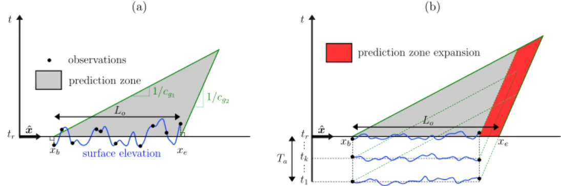
Fig. 1. Evolution of the wave prediction zone in time and space for the assimilation of: (a) spatial data and (b) spatio-temporal data (dash lines are prediction zones boundaries at
time 𝑡𝑘; the increase in the prediction zone relative to that of spatial only observations is highlighted in red); 𝑐𝑔1 and 𝑐𝑔2denote the fastest and slowest group velocities transporting
a significant amount of energy in the wave field, respectively.
The accurate description of a wave field is limited to the knowledge of its wave components energy, which propagates at the wave group velocity. Further, sea states that are of interest in our study, such as described by a JONSWAP wave spectrum, yield a fairly concentrated energy around their peak frequency. This allows using a finite fre-quency bandwidth to describe the evolution of such sea states. Hence, the intersection of the slowest and fastest wave components in the finite frequency bandwidth of the wave field determine the boundary of the spatio-temporal region within which an amount of information suffi-cient to issue a prediction is available. Consequently, as time increases, the accessible prediction region shrinks, to eventually disappear when the assimilated information is completely dispersed. Fig. 1illustrates this phenomenon for a one-directional wave field propagating in the
𝑥-direction. The latest time used in data assimilation corresponds to the reconstruction time 𝑡𝑟 = 𝑡(𝑘=𝐾). When only spatial data are used in the assimilation (i.e., 𝐾 = 1, see Fig. 1a), the prediction zone at reconstruction time(𝑡𝑟)is the spatial area where observations were made. However, when spatio-temporal data sets are acquired (over an assimilation time 𝑇𝑎, seeFig. 1b),
(
𝑡𝑟)expands due to the advection of wave information during 𝑇𝑎.
Therefore, a point(𝑥, 𝑡≥ 𝑡𝑟
)is included in the prediction zone if
𝑥𝑏+ 𝑐𝑔 1 ( 𝑡− 𝑡𝑟)≤ 𝑥 ≤ 𝑥𝑒+ 𝑐𝑔2 ( 𝑡− 𝑡𝑟), (16)
where 𝑐𝑔1and 𝑐𝑔2are the fastest and slowest group velocities, respec-tively, and 𝑥𝑏and 𝑥𝑒define the beginning and the end of
( 𝑡𝑟)(Fig. 1) as ⎧ ⎪ ⎨ ⎪ ⎩ 𝑥𝑏= min 𝑗 ( 𝑥𝑗), 𝑥𝑒= max 𝑗 ( 𝑥𝑗)+ 𝑐𝑔 2𝑇𝑎, (17)
where 𝑥𝑗 are spatial locations of the observations. Although future applications could rely on observations with spatial location variations, i.e., 𝑥𝑗 functions of time, the presented investigations are restricted to
fixed measurement locations.
3.3. Bandwidths of the reconstructed wave field
As mentioned above, the accurate representation of the wave field dynamics can be ensured by selecting a finite wavenumber bandwidth having relevant cutoff limits 𝑘min,max. However, the spatio-temporal
characteristics of the observation grid limit the wave information that is accessible for reconstruction, thus imposing constraints on these cutoffs. For instance, the smallest wavenumber that is measurable in a given grid 𝑘min= 2𝜋∕𝐿
𝑜is function of the largest distance 𝐿𝑜= 𝑥𝑒− 𝑥𝑏
between two observation points at reconstruction time 𝑡𝑟(Fig. 1b). At the same time, 𝑥𝑒is a function of the chosen minimum group velocity
𝑐𝑔
2of individual wave components in the wave field.
When reconstructing a wave field over a uniformly sampled obser-vation grid (i.e., one with constant spatial sampling), the maximum
high cutoff wavenumber must satisfy Shannon’s condition, i.e., 𝑘max≤
2𝜋∕(2𝓁𝑜)where 𝓁𝑜 is the distance between two observation points. However, using an optical sensing method, the observation grid is highly non-uniform, and 𝑘max must be set such that the spectral
en-ergy truncated at higher frequencies be negligible for the dynamic description of the wave field. In later applications, we use 𝑘max =
20𝑘𝑝 <min
𝛥𝑥 (2𝜋∕ (2𝛥𝑥))with 𝛥𝑥 the distance between two consecutive
observation points and 𝑘𝑝the wavenumber of the peak spectral energy.
3.4. Group velocities for the determination of the prediction zone
In applications, the cutoff frequencies calculated as discussed above may be too restrictive to estimate the evolution of the prediction zone, i.e., due to the asymptotic behavior of the wave spectrum as the wavenumber goes to infinity, the high cutoff wavenumber tends to be larger than necessary. Instead, the group velocities 𝑐𝑔1,2 governing the evolution of the prediction zone boundaries are defined on the basis of angular frequencies 𝜔1 and 𝜔2 corresponding to a low and high
minimum energy threshold, respectively, in the wave energy density spectrum as 𝑆𝜂(𝜔1)= 𝑆𝜂 ( 𝜔2)= 𝜇𝑆𝜂 ( 𝜔𝑝), (18)
where 𝑆𝜂(𝜔) is the wave energy density spectrum, 𝜔𝑝 is the peak
angular frequency and 𝜇 ≪ 1 is a small fraction of the peak spectral energy (𝜇 = 0.05 is used throughout the paper). In the following, the linear deep water dispersion relationship is used to estimate the group velocities from 𝜔1,2, i.e., 𝑐𝑔= 𝑔∕ (2𝜔).
4. Experimental and numerical frameworks
Applications presented hereafter are based on surface elevations measured in laboratory experiments and computed in corresponding numerical simulations. Both data sets are referred to full scale wave parameters, but they are both performed at a 𝓁∗ = 1:50 geometric
scale (corresponding time scale is 𝑡∗ = √𝓁∗ ≈ 7.06 under Froude
scaling), for long-crested wave trains generated in the oceanic 3D tank of École Centrale de Nantes (ECN), which is 50 m long, 30 m wide, and 𝑑 = 5 m deep. Waves are generated at one side of the tank by 48 individual rotating flaps, and absorbed by a beach at the other extremity. Numerical simulations are performed using the open-source code HOS-NWT1 developed at ECN. It makes use of the HOS method to simulate a numerical wave tank, and has been extensively used and validated against real wave tank experiments (Bonnefoy et al.,2010;
Ducrozet et al.,2012). Based on a pseudo-spectral approach, the HOS method solves, to an arbitrary order 𝑀 in wave steepness, the nonlinear free surface boundary conditions for a velocity potential. A converged
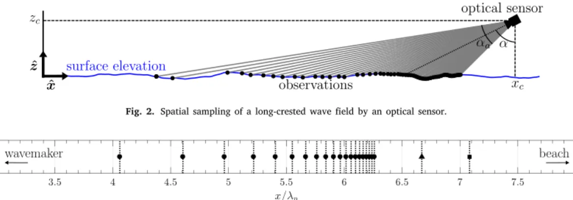
Fig. 2. Spatial sampling of a long-crested wave field by an optical sensor.
Fig. 3. Location of observation wave gauges 1 to 20 (
∙
) and of two additional downstream gauges 21 (▴) and 22 (■). The wavemaker is located at 𝑥∕𝜆𝑝= 0and the beach at 𝑥∕𝜆𝑝≈ 14.86.estimate of the potential (for which a value of 𝑀 = 7 is used hereafter) gives access to the fully nonlinear solution. In Section6, this numerical model is used to improve the analysis pertaining to the experimental results. As waves of characteristic wave steepness larger than 𝐻𝑠∕𝜆𝑝∼
0.035(where 𝜆𝑝= 2𝜋∕𝑘𝑝is the peak wavelength) will start breaking, a
wave breaking model allowing to both detect impending breaking and absorb wave energy is used in HOS-NWT (Seiffert et al.,2017;Seiffert and Ducrozet,2018). The same wavemaker motion is specified in both laboratory experiments and numerical simulations, which ensures a consistent comparison between experimental and numerical results.
In the following, we first detail the experimental and numerical setups used to acquire/compute surface elevation data. An analysis of experimental measurements is then performed through the characteri-zation of noisy perturbations. Finally, we present relevant indicators of the quality of free surface prediction and the procedure implemented to reliably evaluate them.
4.1. Description of the experimental/modeling setups
As shown in Fig. 2, spatial sampling of a free surface elevation by an optical sensor exhibits gaps due to shadowing effects from the illuminated wave fronts and, assuming a uniform distribution of beams over the sensor’s aperture angles, measurement points density geometrically decreases with the distance from the sensor.
In experiments/simulations, free surface elevations are measured/ computed at 22 wave gauges (resistive probes in experiments), irreg-ularly distributed along the wave direction of propagation. Consistent with an optical sensor facing the ‘‘wavemaker side’’ of the tank, the first 20 measurement points have a decreasing density away from it, corresponding to the intersection with a surface of uniformly angularly spaced beams propagating away from a point source (e.g., LIDAR camera). We consider the illumination of a flat surface, which al-lowed us to position the gauges vertically into the water. This way, wave-shadowing effects are not reproduced but only the geometrically decreasing density of observations, which is the prominent source of irregularity in the measurement points locations. The virtual sensor is located at an elevation 𝑧𝑐= 30m (0.6 m in tank scale, 𝑧𝑐∕𝜆𝑝 ≈ 0.19)
and aimed at the water surface with an angle 𝛼 = 76◦and 20 virtual
beams which are uniformly spread over an aperture angle of 𝛼𝑎= 20◦
(seeFig. 2for a representation of 𝛼 and 𝛼𝑎). The resulting geometrical
distribution of the wave gauge locations is depicted in Fig. 3. Two additional gauges measure downstream elevations for comparison with predictions. Every gauge is labeled according to its 𝑥-location, from 1 for that closest to the wavemaker to 22 for that furthest away. Wave gauges provide observations that are used as input to the surface recon-struction and prediction algorithms. The number of spatial observations is thus constant at 𝐽 = 20, and the number of observation times 𝐾 depends on the assimilation time duration 𝑇𝑎and data acquisition time step
τ
as 𝐾 = 𝑇𝑎∕τ
.Table 1
Summary of the targeted and generated full-scale sea states in both experiments and numerical simulations. Each case is labeled in alphabetical order from the smallest to the largest characteristic wave steepness 𝐻𝑠∕𝜆𝑝.
Case Target Experiments Simulations
𝐻𝑠[m] 𝐻𝑠∕𝜆𝑝[%] 𝐻𝑠[m] 𝐻𝑠∕𝜆𝑝[%] 𝐻𝑠[m] 𝐻𝑠∕𝜆𝑝[%] A 1.00 0.64 0.89 0.57 1.01 0.65 B 2.00 1.28 1.86 1.19 2.02 1.29 C 3.00 1.92 2.81 1.80 3.02 1.93 D 4.00 2.56 3.79 2.43 4.01 2.57 E 5.00 3.20 4.64 2.97 4.98 3.18 F 6.00 3.84 5.60 3.59 5.87 3.76 G 7.00 4.48 6.46 4.14 6.69 4.28 H 9.00 5.76 8.02 5.13 8.06 5.16
In both experiments and numerical simulations, we consider a full-scale one-directional wave field extracted from a JONSWAP spectrum with a 𝑇𝑝 = 10 s peak period (≈ 1.41 s in tank scale) and a 𝛾 = 3.3peakedness parameter. Eight sea-states were generated using the same set of wave phases (Table 1), with their significant wave height
𝐻𝑠= 𝐻𝑚0 = 4 √
𝑚0(where 𝑚0 =∫0+∞𝑆𝜂(𝑓 ) d𝑓) selected such that the
characteristic steepness 𝐻𝑠∕𝜆𝑝varies between ∼ 0.6% and ∼ 5%, with
𝜆𝑝≈ 156m (3.12 m in tank scale). In tank scale we have 𝜆𝑝< 𝑑, which
confirms that the deep water approximation is applicable.
A theoretical wavemaker motion is deduced by applying a transfer function based on the one-directional finite-depth linear wavemaker theory and on the wavemaker geometry, which is, for both experiments and simulations, a rotating flap that is hinged three meters below the mean surface level. The amplitude of the wavemaker deflection is ad-justed according to the target 𝐻𝑠values. Without further consideration,
the obtained theoretical motion serves as input for our physical and numerical wavemakers.
We notice differences between the target and generated significant wave heights (refer to Section4.2for the explicit formulation Eq.4.2
for the calculation of 𝐻𝑠). In experiments, 𝐻𝑠 values are found con-sistently lower than target values. For sea states of small to moderate steepness (cases A to D), this is mainly explained by the wavemaker transfer function leading the physical wavemaker to generate waves of lower amplitude than according to the input. In contrast, simulations yield 𝐻𝑠values that are slightly higher than the targets by an amount
that is of the same order of magnitude as the expected effect pertaining to the wave reflection on the beach (i.e., lower than 1%). Since the numerical beach is set such that its reflection rate corresponds to the physical one, wave reflection is expected to have a similar effect on the experimental results, i.e., very limited. For high steepness, i.e., 𝐻𝑠∕𝜆𝑝≳
3.5%(cases E to H), wave breaking events appear, dissipating energy and reducing our estimates of 𝐻𝑠. Wave-breaking dissipation is
encoun-tered in both experiments and simulations due to the wave breaking modeling in the numerical model.
Fig. 4. Time series of surface elevation measured in experiments at gauge 22 for case E (Table 1). Three characteristic times are marked on the record, 𝑡𝑎: all the generated wave components have been measured at all gauges; 𝑡𝑏: shutdown of the wavemaker; 𝑡𝑐: all the generated wave components have propagated past all gauges.
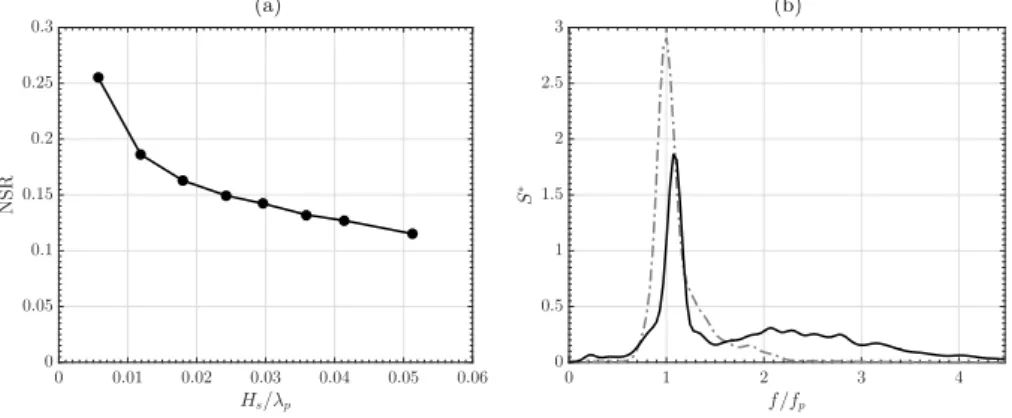
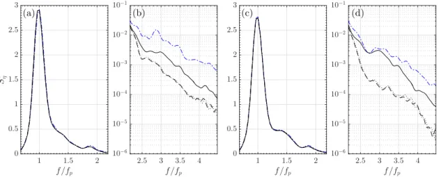
Fig. 5. (a) Noise amplitude to wave amplitude ratio as a function of characteristic wave steepness, and (b) normalized noise ( ) and wave ( ) spectra averaged over
all the characteristic wave steepnesses.
Fig. 6. Normalized surface elevations for case A at the locations of gauges 1 to 22. Components of frequency higher than 1.4𝑓𝑝has been removed using a low-pass filter.
4.2. Analysis of experimental data
Fig. 4shows a typical time series of surface elevation measured at a resistive probe in laboratory experiments. Time 𝑡 = 0 corresponds to the start of the wavemaker motion, i.e., the beginning of wave generation. At time 𝑡𝑎, it is estimated based on a truncation of the prescribed
wave energy spectrum (similar to Section 3.4) that all the energetic wave components generated at the wavemaker have been seen by all gauges. At time 𝑡𝑏, the wavemaker is shutdown and waves generation
is interrupted. Finally, similar to the determination of 𝑡𝑎, at time 𝑡𝑐, it is estimated that all the generated energetic wave components have propagated past all gauges. Based on this, the data used for the wave field prediction study is restricted to the time interval [𝑡𝑎, 𝑡𝑏], with
𝑡𝑏− 𝑡𝑎≈ 173𝑇𝑝.
It is desirable to analyze and quantify the influence of the perturba-tions pertaining to the limitaperturba-tions of our experimental setup (referred to as ‘‘noise’’ throughout this work) on the recorded wave signal. This is done by considering that the rest of the data acquired at wave gauges, for a few dozen peak wave periods beyond 𝑡 = 𝑡𝑐, provides
a representation of noise during the entire data acquisition duration. Based on this data, a noise to signal ratio NSR = 𝐻𝑛∕𝐻𝑠is computed as a function of characteristic heights for both the primary wave (𝑡 ∈ [
𝑡𝑎, 𝑡𝑏]) and noise (𝑡≥ 𝑡𝑐) signals following
⎧ ⎪ ⎨ ⎪ ⎩ 𝐻𝑠= 1 𝑁𝑝 ∑𝑁𝑝 𝑗=14 𝜎𝜂 ( 𝑥𝑗, 𝑡𝑎≤ 𝑡 ≤ 𝑡𝑏 ) , (a) 𝐻𝑛= 1 𝑁𝑝 ∑𝑁𝑝 𝑗=14 𝜎𝜂 ( 𝑥𝑗, 𝑡≥ 𝑡𝑐 ) , (b) (19)
respectively, where 𝜎𝜂(𝑥, 𝑡)denotes the standard deviation of the free
surface elevation 𝜂 (𝑥, 𝑡) and 𝑁𝑝 = 22wave gauges. The NSR is
com-puted for each case A to H inTable 1and plotted inFig. 5a as a function of the corresponding characteristic wave steepness. We see that the NSR decreases as a function of wave steepness, with the largest value being about 25% for the smallest steepness and the smallest value being about 11.5% for the largest steepness. It thus appears that the geometry of our experimental set-up, in a 3D wave tank allowing the generation of directional wave fields, may have significantly affected the targeted one-directional wave fields. As will be detailed in Section6.3, this po-tentially large NSR may affect the performance of the wave prediction algorithm.
To better quantify noise effects on the desired experimental data and relate the generated noise to a physical process, we computed the power spectral density 𝑆𝑛 of the noisy part of the signal (𝑡≥ 𝑡𝑐). For
each steepness, the spectrum was averaged over results obtained at the 22 wave gauges and normalized as 𝑆∗
𝑛 = 𝑆𝑛𝑓𝑝∕𝑚0, where 𝑚0 =
𝐻𝑛2∕16is the zeroth-order moment of the spectrum. These normalized noise spectra were found to be nearly identical for each steepness.
Fig. 5b shows their average, which is composed of a narrow-banded peak, centered on ∼ 1.1𝑓𝑝, and a broad-banded high frequency part of much lower amplitude. The wave spectrum, calculated on[𝑡𝑎, 𝑡𝑏], is given on the same figure as a visual help for interpretation.Fig. 6
shows normalized surface elevations of the noise signal 𝜂∕𝐻𝑛in which
frequencies 𝑓 > 1.4𝑓𝑝 have been removed by filtering, i.e., these correspond to the dominant part of the noise signal. It shows that
Fig. 7. Each sample consists of a time trace from the same generated surface
realization. They can be partially overlapping, separated by a time span 𝛥𝑡 from their neighbors.
elevations for case A at wave gauges 1 to 22 (which are aligned along the 𝑥-direction) are mostly in phase, suggesting that the dominant experimental noise may be caused by resonant excitations of transverse modes in the 3D wave tank. This hypothesis is confirmed by our visual observations of these waves during calm-down times between measure-ments, and is explained by the presence of small interstices between the wavemaker flaps, locally generating transverse disturbances. The much less energetic noisy components of the signal, with frequencies
𝑓 > 1.4𝑓𝑝, were not found to be in phase, indicating that they result
from aleatory processes.
4.3. Misfit indicators definitions
The misfit indicator used to quantify the accuracy of the predicted wave field is defined as
(𝑥, 𝑡) = 1 𝑁𝑠 𝑁𝑠 ∑ 𝑖=1||𝜂 𝑖(𝑥, 𝑡) − 𝜂r𝑖(𝑥, 𝑡)|| / 𝐻𝑠, (20)
where 𝜂 is the predicted surface elevation and 𝜂r is the reference surface (measured or calculated, depending on whether experimental or numerical data is used). To better assess its overall behavior, the misfit is averaged over 𝑁𝑠surface samples, denoted by index 𝑖. An unbiased
estimate can only be obtained for a large number of samples from independent wave field realizations (i.e., of different sets of random wave phases) with, to the limit, 𝑁𝑠 → ∞. Instead, we elected to
generate one single surface realization per sea state, but to record or compute wave gauge data over a long time so that the signals can be split into a sufficiently large number of samples of meaningful duration
𝑇𝑎. Additionally, the number of samples is increased by selecting them as partially overlapping, i.e., shifting them in time by 𝛥𝑡 < 𝑇𝑎, as illustrated in Fig. 7. Therefore, the information used to estimate the misfit is the surface elevation data in the total time window covered by the samples, which has a duration 𝑇𝑐= 𝑇𝑎+(𝑁𝑠− 1)𝛥𝑡. A similar approach was employed in Naaijen et al. (2014) to investigate the spatio-temporal evolution of the prediction zone based on experimental and numerical data. The wave field prediction error at a specific location 𝑥 is finally computed by averaging the corresponding misfit over the theoretical time-prediction zone 𝑡 ∈[𝑡min, 𝑡max]as
(𝑥) = 1
𝑡max− 𝑡min∫
𝑡max
𝑡min (𝑥, 𝑡) d𝑡. (21)
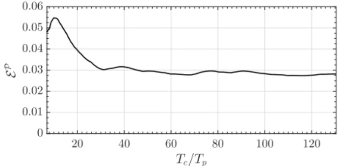
Fig. 8shows, for case E, the evolution of the wave field prediction errorcomputed as a function of the amount of data used to calculate
it, quantified by the relative duration 𝑇𝑐∕𝑇𝑝 of the time window used to evaluate the misfit. We see that the prediction error converges for
𝑇𝑐∕𝑇𝑝 ∼ 60. Note that the wave gauge network used to generate the
observations covers a zone only slightly larger than 2𝜆𝑝. If this zone was larger, the optimal number of peak wave periods for the sampling time window would likely be less than 60.
Additionally, for deterministic comparison, we make use of the cross-correlation between time series corresponding to the predicted and the measured surface elevations, which provides a correlation factor 𝐶 as a function of a time-lag . The maximal value of the correlation factor and its corresponding time-lag can be interpreted as the correspondence in terms of shape and amplitude of the two
Fig. 8. Nonlinear (ICWM) prediction error estimate at the location of gauge 22 as
a function of the length of the time window used to evaluate the misfit, 𝑇𝑐 = 𝑇𝑎+
( 𝑁𝑠− 1
)
𝛥𝑡, normalized by the peak spectral period 𝑇𝑝, and in which 𝛥𝑡∕𝑇𝑝≈ 0.07. Here, 𝑇𝑎∕𝑇𝑝≈ 7andτ∕𝑇𝑝≈ 0.07, and simulated reference data from case E are used.
elevations, and as an estimate of the time shift between the two elevations, respectively. The cross-correlation is defined by
𝐶( ) = 1
𝑡max− 𝑡min∫
𝑡max 𝑡min
𝜂∗(𝑡) × 𝜂∗r(𝑡 + ) d𝑡, (22) where 𝑡min,max are the prediction zone boundaries and 𝜂∗(𝑡) =
𝜂(𝑡) ∕𝜎𝜂
(
𝑡min≤ 𝑡 ≤ 𝑡max)is the normalized free surface elevation
(sim-ilarly, 𝜂∗
r = 𝜂r∕𝜎𝜂r for the reference surface).
5. Prediction error sensitivity to reconstruction algorithm
We first assess the sensitivity of the prediction error to both the method used (linear or nonlinear) and parameters of the assimilation procedure, namely the assimilation time 𝑇𝑎and the time shift of the assimilated data
τ
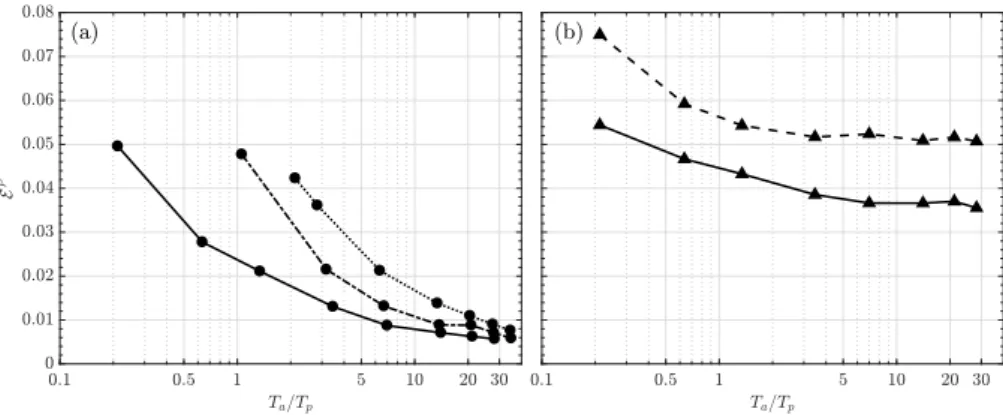
.For case A, which corresponds to a mild characteristic wave steep-ness of 0.65%,Fig. 9a shows that the linear prediction error converges well as 𝑇𝑎increases, for the three considered
τ
values, althoughconver-gence is slower for larger
τ
. Hence, the converged error is independent of the time resolution of observations. This is a consequence of the characteristics of the physical description emerging from observations. As the assimilation time increases, the diversity of wave processes included in the assimilated information is enhanced, with respect to the relevant physics simulated in the model, causing the prediction error to converge. Additionally, the accuracy of the description of physical phenomena, which is directly function of the time resolution of observations, affects the prediction error convergence rate: for a given assimilation time 𝑇𝑎, a smaller time stepτ
will yield a prediction errorcloser to the converged value. For the predictions presented later, we keep
τ
∕𝑇𝑝≈ 0.07.For case E, which corresponds to a larger wave steepness of 3.18% and hence a fairly nonlinear case,Fig. 9b shows that, overall, pre-diction errors are larger than for case A, increasing from [0.005, 0.05] to [0.05, 0.075]. Fig. 9b also shows that, as could be expected for this nonlinear case, the prediction errors are larger with the linear method than with the nonlinear method. Finally, the convergence of the nonlinear method to achieve an approximately constant value of
𝜀requires a slightly larger 𝑇𝑎than for the linear method. This can be
explained by the higher level of physics represented in the ICWM model than in LWT, which requires larger time scales to achieve convergence.
6. Prediction results and discussion
Applications of the reconstruction and forecasting algorithms to cases ofTable 1are presented in the following and the accuracy of the wave field forecast is discussed, in particular, in terms of its sensitivity to the linear or nonlinear methods used.
Fig. 9. Prediction error at the location of gauge 22 as a function of the normalized assimilation time 𝑇𝑎∕𝑇𝑝in case (a) A (
∙
) and (b) E (▴). In case A, the linear error is plotted forτ∕𝑇𝑝≈ 0.07( ), 0.35 ( ) and 0.71 ( ). In case E, a time stepτ∕𝑇𝑝≈ 0.07is used and both the linear (LWT, ) and nonlinear (ICWM, ) errors are plotted. Simulated reference data is used in both figures.6.1. Wave group analysis
All cases in Table 1 correspond to sea states generated using a JONSWAP spectrum with identical peak period 𝑇𝑝= 10s (at full scale)
and peakedness 𝛾 = 3.3, but a different significant wave height 𝐻𝑠and,
hence, characteristic wave steepness 𝐻𝑠∕𝜆𝑝. In both the physical and numerical wave tanks, these sea states are generated using the same set of random phases, so time series of surface elevations should be similar, except for small changes in amplitude due to nonlinear effects, proportional to 𝐻𝑠.
In the following, we analyze the prediction error for a group of 8 waves of elevation on the order of 𝜂 ∼ 0.5𝐻𝑠 approximately
cen-tered at 𝑡 = 113𝑇𝑝, recorded/simulated at wave gauge 22 for cases
A to H (see Fig. 4). The data used in the prediction algorithms was selected for the prediction zone to span 𝑡 ≈ 108𝑇𝑝 to 118𝑇𝑝 at the location of gauge 22. Fig. 10shows time series of surface elevations for these wave groups in cases A, E and H, compared to predictions of the linear (LWT), linear corrected (LWT-CDR), and nonlinear (ICWM) models, using experimental (a, c, e) and numerical (b, d, f) data. For each case, only small differences due to experimental noise can be seen between the experimentally and numerically generated reference surfaces. While there is an overall agreement between the reference and predicted surfaces, differences in wave phase and elevation increase with wave steepness, due to cumulative effects of nonlinearity during wave propagation. Accordingly, for the smallest wave steepness (case A), all three models predict the same surface elevation, in good agree-ment with references, particularly for numerical data (b) for which predictions almost perfectly overlap the HOS solution, but predictions become increasingly different between the three algorithms, the larger the characteristic wave steepness. Although differences do not appear visually large, this is more pronounced for the algorithm based on ICWM, which, as will be shown next using various prediction error metrics, provides the most accurate prediction.
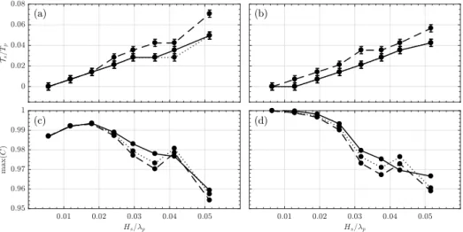
Differences between the reference (measured or simulated with HOS) surface elevations and those predicted by the three algorithms are quantified by their maximum cross-correlation max(𝐶) (i.e., normalized convolution, Eq. (22)) and corresponding time-lag 𝑠 = arg max (𝐶).
Both parameters are shown in Fig. 11for all cases inTable 1, based on time series measured or simulated at the location of wave gauge 22 (e.g.,Fig. 10). The former quantifies the accuracy of the prediction in terms of wave shape and amplitude, while the latter quantifies the time-shift of the predicted signal compared to the reference signal.Fig. 11a, b show that, for all prediction algorithms, time-lag increases with wave steepness (i.e., nonlinearity), from 0 for the smallest steepness to a few percent of 𝑇𝑝 for the largest one, consistent with the expected
effects of nonlinearity. As seen for instance in the time series ofFig. 10, LWT yields the largest time-lags compared to the nonlinear models.
LWT-CDR, which includes a phase shift correction, provides a time-lag very close to that of ICWM, particularly for the simulated data, indicating that the nonlinear phase shift prevails over the nonlinear wave geometry represented in the latter model for these cases. Also, the rate of increase of time-lag with wave steepness is similar whether or not the nonlinear phase shift is included in the model. This result is unexpected since this phase shift its due to nonlinear amplitude dispersion, which is function of wave steepness.
Fig. 11c, d show the maximum cross-correlations for the same cases. Consistent with the larger time-lag, max(𝐶) mostly decreases, the larger the wave steepness, to reach a minimum of 96% for the largest wave steepness. Except for case G, which is discussed below, the maximum cross-correlation is larger using ICWM, which is expected since only this model is able to represent nonlinear wave geometry. The abnormal behavior of case G, which is seen in both the experimental and numerical data, likely results from a significant increase in wave breaking events within the considered wave group for this case. Note, for case H, which has an even larger steepness, wave phases were such that breaking was not as widespread as for case G. Wave breaking affects wave geometry in a non-trivial manner and is not represented in ICWM. In the case of the wave group considered here, for some unknown reason, it appears that broken waves are better represented in the linear model than using ICWM.
Finally,Fig. 12shows results similar toFig. 11, using ICWM for numerical or experimental data, at wave gauges 20, 21 and 22. Ob-servations are acquired (and reconstructed) at wave gauge 20, which is the last gauge used in observations, and predictions are made at the other 2 gauges, which are increasingly distant from it (Fig. 3). For both the experimental and numerical data, the time-lags and their rates of increase with wave steepness are lower for prediction locations closer to the observation gauge (Fig. 12a, b). This results from inaccuracies in nonlinear wave propagation modeled by ICWM, which yield increasing differences in predicted surface elevations with time or space trav-eled, compared to the reference data. Consistent with this observation,
Fig. 12c, d show that, for steepnesses larger than ∼ 2.5%, the maximum cross-correlation decreases as the distance of the prediction gauge to the observation location increases.
6.2. Instantaneous misfit of wave prediction
We investigate next the evolution of the instantaneous misfit (𝑥, 𝑡) of the wave prediction for case E, which corresponds to a moderate steepness, although nonlinear effects already have a marked influence on the wave field dynamics. For both experimental and numerical cases, we compare the misfit obtained using the LWT, LWT-CDR and ICWM prediction algorithms.
Fig. 13shows the temporal evolution of the wave prediction misfit computed using different algorithms, with respect to data simulated
Fig. 10. Time series of surface elevations measured/simulated at gauge 22 for a group of 8 waves ( ) for cases: (a, b) A, (c, d) E and (e, f) H, of increasing nonlinearity. Predicted surface elevations are shown for the: linear (LWT, ), corrected linear (LWT-CDR, ), and nonlinear (ICWM, ) models. Left (a, c, e): experiments; right (b, d, f): simulations.
Fig. 11. Normalized time-lag (a, b) and maximum cross-correlation (c, d) computed for cases inTable 1, based on reference time series measured (left column)/simulated with HOS (right column) at the location of wave gauge 22 for wave groups similar to those inFig. 10, based on: linear (LWT, ), corrected linear (LWT-CDR, ), and nonlinear (ICWM, ) prediction algorithms. Error bars in (a, b) result from the resolution of the time series..
Fig. 12. Normalized time-lag (a, b) and maximum of cross-correlation (c, d) for the nonlinear (ICWM) predictions, at the location of gauge 20 (■), 21 (▴) and 22 (
∙
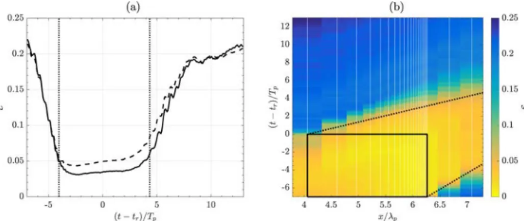
). Left (a, c): experiments; right (b, d): simulations. Error bars on (a, b) correspond to the time resolution of the time series.Fig. 13. Time evolution of wave prediction misfit, computed with respect to data simulated for case E: (a) at gauge 22 using the linear (LWT, ) and nonlinear (ICWM, ) prediction algorithms; (b) for all gauges using the nonlinear (ICWM) prediction algorithm (black rectangle encompasses assimilated observations; data was collected at gauges’ 𝑥-locations (vertical lines) and interpolated using the nearest neighbor method). In each subfigure, dotted lines ( ) mark the prediction zone boundaries.
for case E, at both gauge 22 (a) and for all gauges (b). The misfit at gauge 22 is significantly lower within the accessible prediction zone, [
𝑡min, 𝑡max](Fig. 13a), reaching a minimum value of about 3.5% for ICWM, compared to about 4.5% for LWT, whose misfit is consistently about 30% larger than that of ICWM. Within the time prediction zone, the error gradually slightly increases due to the limited physics repre-sented in both wave models. In the spatio-temporal domain (Fig. 13b), ICWM’s misfit is lowest within the theoretical prediction zone, reaching a maximum of about 7% along its boundary. As the 𝑥-location of the wave gauge increases, the misfit gradient decreases across the predic-tion zone upper boundary 𝑡max, or in other words the transition of the
misfit values from within to outside the prediction zone becomes more diffused, which is due to the dispersion of the assimilated information. More specifically, as detailed in Section 3.2, the energy associated with the reconstructed wave components disperses as 𝑥 increases, gradually limiting the physical description of the wave field. Even within the spatio-temporal region corresponding to the observations (black rectangle inFig. 13b), the misfit is non-zero since observations are discrete rather than continuous samples of elevations. Hence, the reconstructed elevation (nowcast) is always an estimate of the reference solution. Note that the accessible prediction horizon in the depicted configuration is 𝑡max − 𝑡
𝑟 ≈ 3.7𝑇𝑝 and 4.3𝑇𝑝 at gauges 21 and 22,
respectively, and is expected to further increase at larger distances (at the expense of the prediction accuracy). Then, from the location where the beginning of the prediction zone 𝑡min matches the reconstruction
time 𝑡𝑟, the accessible horizon starts decreasing.
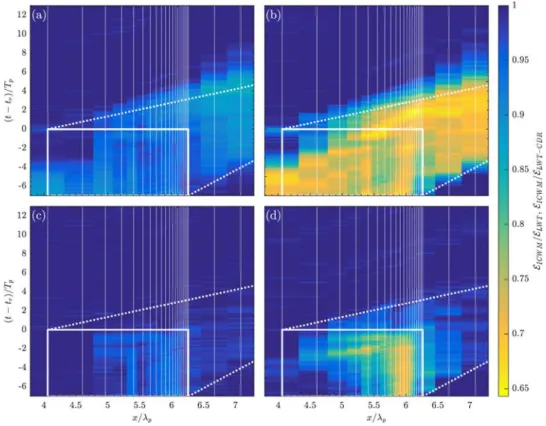
For the same case E,Fig. 14shows for both experimental or sim-ulated reference data, the spatio-temporal evolution of the ratio of the nonlinear (ICWM) to linear (LWT; a, b) or linear with corrected dispersion (LWT-CDR; c, d) wave prediction misfit. For the simulated data (Fig. 14b), the misfit is reduced by up to ∼ 35% within the predic-tion zone when using ICWM instead of LWT. Compared to LWT-CDR (Fig. 14d), the reduction is smaller and mostly limited to the spatio-temporal region of assimilated data (within the solid box), particularly where the wave gauge density is larger. Outside of this region (𝑡 > 𝑇𝑎≈
7𝑇𝑝; time propagation) or at the location of gauges 21 and 22 (space propagation), the misfit ratio rapidly approaches one, indicating that the improvement achieved using ICWM rather than LWT-CDR becomes negligible. For the experimental data (Fig. 14a, c), similar patterns are observed, but the improvement achieved using ICWM is not as pronounced as for simulated data.
These results indicate that the improved representation of nonlin-ear wave geometry using ICWM mostly affects the accuracy of the reconstructed part of the wave field. Once reconstructed waves are propagated to the prediction zone, the nonlinear phase shift, which is corrected in LWT-CDR to the same level as in ICWM, becomes the main source of error and effects of nonlinear wave geometry become
negligible compared to it. The wave models are parameterized to provide a relevant and consistent approximation of the wave field over the entire region covered by the observations. Hence, while the reconstructed wave field is constrained to fit the measurements, when waves are propagated to issue a prediction, only their propagation properties featured in the models come into play.
6.3. Influence of experimental noise on wave prediction
The prediction misfits based on numerical and experimental refer-ence data are compared inFig. 15, at gauges 20, 21, and 22, for all cases listed inTable 1, using the linear (LWT) or nonlinear (ICWM) algorithms. To better assess the effect of experimental noise on the prediction misfit, a ‘‘noisy numerical dataset’’ was created by adding to the numerical data a noise signal having the same spectral shape (or NSR) as that analyzed for the experiments (Fig. 5b), scaled by the measured noise amplitude 𝐻𝑛 (Fig. 5a), with independent random
phases for each wave gauge. As would be expected, for both algorithms, the prediction misfits are larger at all wave gauges using experimental data, as compared to noise-free numerical data, particularly for cases with a lower steepness, which have relatively larger noise levels. Using the noisy numerical data, however, prediction misfits increase to nearly match those of the experimental data. This indicates that the noisy numerical data is consistent with the experimental data and provides a
digital twinof experiments that explains, for the most part, differences observed between predictions issued for experimental and noise-free numerical data.
6.4. Application to remote sensing: free surface slope prediction
In the free surface elevation predictions described above, the nonlin-ear phase correction was responsible for the main relative improvement in prediction misfit, rather than the nonlinear wave geometry rep-resented in ICWM. While for many ocean engineering applications predicting instantaneous free surface elevations is most important, such as when computing wave forces or runup on structures, or controlling a wave energy converter, in some applications such as remote sensing the main parameter of interest is free surface slope, which governs the backscattered signal to the radar or optical sensor used (e.g.,
Nouguier et al., 2010, 2014). Hence, in the following, we quantify the improvement in free surface slopes representation achieved using ICWM rather than LWT-CDR. More specifically, at the location of wave gauge 20, we analyze the evolution as a function of wave steepness of the maximum prediction misfit ratio
𝐼 𝐶𝑊 𝑀∕𝐿𝑊 𝑇 −𝐶𝐷𝑅, for both