HAL Id: hal-01723223
https://hal.archives-ouvertes.fr/hal-01723223
Submitted on 5 Mar 2018
HAL is a multi-disciplinary open access
archive for the deposit and dissemination of sci-entific research documents, whether they are pub-lished or not. The documents may come from teaching and research institutions in France or abroad, or from public or private research centers.
L’archive ouverte pluridisciplinaire HAL, est destinée au dépôt et à la diffusion de documents scientifiques de niveau recherche, publiés ou non, émanant des établissements d’enseignement et de recherche français ou étrangers, des laboratoires publics ou privés.
Statistics versus Machine Learning
Danilo Bzdok, Naomi Altman, Martin Krzywinski
To cite this version:
Danilo Bzdok, Naomi Altman, Martin Krzywinski. Statistics versus Machine Learning. Nature Meth-ods, Nature Publishing Group, 2018, 15, pp.233-234. �hal-01723223�
POINTS OF SIGNIFICANCE
Statistics versus Machine Learning
Statistics draws population inferences from a sample and machine learning finds generalizable predictive patterns.
Two major goals in the study of biological systems are inference and prediction. Inference creates a mathematical model of the data-generation process to formalize our understanding or test a hypothesis about how the system behaves. Prediction aims at
forecasting unobserved outcomes or future behavior, such as whether a mouse with a given phenotype will have a disease. Prediction makes it possible to identify best courses of action (e.g. treatment choice) without requiring understanding of the underlying mechanisms. In a typical research project, both inference and prediction are of value— we want to know how biological processes work and what will happen next. For example, we might want to infer which biological processes are associated with the dysregulation of a gene in a disease as well as classify whether a subject has the disease and predict the best
therapy, such as drug intervention or invasive surgery.
Many methods from statistics and machine learning (ML) may, in principle, be used for both prediction and inference. However, statistical methods have a longstanding focus on inference, which is achieved by devising and fitting a project-specific probability model. The model allows us to compute a quantitative measure of confidence that a discovered relationship describes a “true” effect that is unlikely to be result from noise. Furthermore, if enough data are available, we can explicitly verify assumptions (e.g. equal variance) and refine the specified model, if needed.
By contrast, ML concentrates on prediction by using general-purpose learning algorithms to find patterns in often rich and unwieldy data [1,2]. ML methods are particularly helpful when the number of input variables exceeds the number of subjects: “wide-data”, in contrast to “long-data”, where the number of subjects is larger than input
variables. ML methods make minimal assumptions about the data-generating system. They can be effective even when the data are gathered without carefully controlled experimental design and in the
presence of complicated non-linear interactions. However, despite convincing prediction results, the lack of an explicit model can make ML solutions difficult to directly relate to existing biological
knowledge.
Classical statistics and ML vary in computational tractability as we increase the number of variables per subject. Classical statistical modeling was designed for data with a few dozen input variables and sample sizes that would be considered small to moderate today. In this scenario, the model fills in the unobserved aspects of the system. However, as the number of input variables and possible associations among them increases, the model that captures these relationships becomes more complex. Consequently, statistical inferences become less precise and the boundary between statistical and ML approaches becomes hazier.
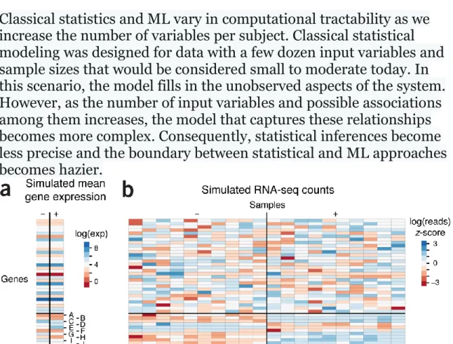
Figure 1 | Simulated expression and RNA-seq read counts for 40 genes in which the
last 10 genes (A−J) are differentially expressed across two phenotypes (−/+). Simulated quantities and heatmaps are log scaled. (a) Simulated log mean
expression levels for the genes generated by sampling from the Gaussian distribution N(4,2). In the + phenotype the differential expression of genes A−J is created by adding N(0,1) to their expression in the – phenotype. (b) The simulated RNA-seq read counts for 10 observations in each phenotype generated from an over-dispersed Poisson distribution based on mean expression in (a) with biological variation. The heatmap shows z-scores of the read counts normalized across all 20 mice for a given gene.
To compare traditional statistics to ML approaches, we’ll use a simple simulation of the expression of 40 genes in two phenotypes (−/+). Gene expression will vary across subjects, but we’ll set up the
simulation so that this variation for the first 30 genes is not related to phenotype. The last 10 genes will be dysregulated, with systematic
differences in mean expression between phenotypes. To achieve this, each gene is assigned an average log expression that is the same for both phenotypes. The dysregulated genes (31−40, labelled A−J) have their mean expression perturbed in the + phenotype (Fig. 1a). Using these average expression values, we simulate an RNA-seq experiment in which the observed counts for each gene are sampled from a
Poisson distribution with mean exp(x + ε) where x is the log average expression, unique to the gene and phenotype, and ε ~ N(0,0.15) acts as biological variability that varies from sample to sample (Fig. 1b). For genes 1−30, which do not have differential expression, the z-scores are approximately N(0,1). For the dysregulated genes, which do have differential expression, the z-scores in one phenotype tend to be positive while the z-scores in the other tend to be negative.
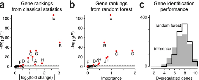
Figure 2 | Gene ranking analysis from classical inference and ML. (a) Unadjusted P
values from statistical differential expression analysis as a function of effect size, measured by fold-change in expression. (b) P values from (a) as a function of gene importance from random forest classification (c) Distribution of the number of dysregulated genes correctly identified in 1,000 simulations by inference (grey fill) and random forest (black line).
Our goal is to determine from the RNA-seq simulation which genes are associated with the abnormal phenotype. We’ll formally test the null hypothesis that the mean expression differs by phenotype based on a widely used generalized linear negative binomial model, which allows for biological interpretability. We’ll do a test for each gene and identify those that show statistically significant differences in mean expression based on P values adjusted for multiple testing using Benjamini-Hochberg [3]. In an alternative Bayesian approach, we
would compute the posterior probability of having differential expression specific to the phenotype.
Figure 2a shows the P value of the tests between phenotypes as a function of the log fold-change in the gene expression. The 10
dysregulated genes are highlighted in red; our inference flagged 9 out of 10 of them (except F, with the smallest log fold-change) as
significant with adjusted P < 0.05. We could use the fold-change as a measure of effect size, with a confidence interval or highest posterior region used to indicate the uncertainty in the estimate. In a realistic setting, genes identified by the analysis would then be validated experimentally or compared to other data sources such as proposed gene networks or annotations.
To ask a similar biological question using ML, we would typically try several algorithms evaluated using cross-validation on independent test mice [3], or bootstrap methods with “out-of-sample” evaluation [4] to select one with good prediction accuracy. Let’s use a random forest (RF) classifier [4], which simultaneously considers all genes and grows multiple decision trees to predict the phenotype without assuming a probabilistic model for the read counts. We show the result of RF with 100 trees in Figure 2b, where the P values from the classical inference are plotted as a function of feature importance weighing each gene. This score quantifies a given gene’s contribution to the average decrease in the tree-forking criterion [5] within a partition when the tree is split selecting that gene. Many ML
algorithms have analogous measures allowing some quantification of the contribution of each input variable to the classification. In our simulation, 8/10 genes with the largest importance measure were from the dysregulated set. Not in the top 10 were the Genes D and F, which had the smallest fold-change (Fig. 2a).
If we perform the simulation 1,000 times and count the number of dysregulated genes correctly identified by both approaches - either based on classical null-hypothesis rejection with an adjusted P value cutoff or predictive pattern generalization with RF and top 10 feature importance ranking—then we find that both methods yield
comparable results. The average number of dysregulated genes identified is 7.4/10 for inference and 7.7 for RF. (Fig. 2c). Both methods have a median of 8/10 but we find more instances of
simulations for which only 2−5 dysregulated genes were identified with inference. This is because the way we’ve designed the selection process is different for the two approaches: inference selects by an adjusted P value cutoff so that the number of selected genes varies, whereas in the RF we select the top 10 genes. We could have applied a cutoff on the importance score, but the scores do not have an
objective scale on which to base the cut.
We’ve been able to use preexisting knowledge about the RNA-seq protocol to design a statistical model of the process and draw inference to estimate unknown parameters in the model from the data. In our simulation, the model encapsulates the relationship between the mean number of reads (the parameter) for each gene for each phenotype and the observed read counts for each mouse. The output of the statistical analysis is a test statistic for a specific hypothesis or an estimate and confidence bounds of the parameter (or a function of the parameter such as the mean fold change). In our example, the model’s parameters relate explicitly to molecular aspects of gene expression—the counts of molecule produced at a certain rate in a cell can be directly interpreted.
To apply ML, we didn’t need to know any of the details about RNA-seq measurements—all that matters is which genes are more useful at discriminating phenotypes based on gene expression. This
generalization greatly helps when we have a large number of variables, such as in a typical RNA-seq experiment that may have hundreds to hundreds of thousands of features (e.g. transcripts)but a much smaller sample size.
Now consider a more complicated experiment in which each
individual subject contributes multiple observations from different tissues . Even if we only conduct a formal statistical test that
compares the two phenotypes for each tissue, the multiple testing problem is greatly increased. The increase in data complexity may make classical statistical inference less tractable. Instead a ML
approach could be used such as clustering of either genes or tissues or both to extract the main patterns in the data, classify subjects, and make inferences about the biological processes that give rise to the phenotype. To simplify the analysis, we could perform a dimension
reduction such as averaging the measurements over the 10 mice with each phenotype for each gene and each tissue.
The boundary between statistical inference and ML is subject to intense debate [1]—some methods fall squarely into one domain but many are used in both approaches. For example, the bootstrap [6] can be used for both statistical inference to improve sampling but also acts as the basis for ensemble methods, such as the RF algorithm. Statistics asks us to choose a model incorporating our knowledge of the system and ML requires us to choose a predictive algorithm by relying on its empirical capabilities. Justifying a model for inference typically rests on whether we feel it adequately captures the essence of the system. The choice of pattern-learning algorithms often rests on measures of past performance in similar scenarios. Inference and ML are complementary in pointing us to biologically meaningful conclusions.
COMPETING FINANCIAL INTERESTS
The authors declare no competing financial interests.
Danilo Bzdok, Naomi Altman & Martin Krzywinski 1. Bzdok, D. Front. Neurosci. 11, 543 (2017).
2. Bzdok, D., Krzywinski, M. & Altman, N. Points of significance: Machine learning: a primer. Nat. Methods 14, 1119–1120 (2017).
3. Krzywinski, M. & Altman, N. Points of significance: Comparing samples — Part II — Multiple testing. Nat. Methods 11, 355–356 (2014).
4. Altman, N. & Krzywinski, M. (2017) Points of Significance:
Ensemble Methods - Bagging and Random Forest. Nat. Methods, 14, 933−934 (2017).
5. Krzywinski, M. & Altman, N. Points of significance: Classification and regression trees. Nat. Methods 14, 757–758 (2017).
6. Kulesa, A., Krzywinski, M., Blainey, P. & Altman, N. Points of
significance: Sampling distributions and the bootstrap. Nat. Methods, 12, 477−478 (2015).
Danilo Bzdok is an Assistant Professor at the Department of
Psychiatry, RWTH Aachen University, in Germany and a Visiting Professor at INRIA/Neurospin Saclay in France. Martin Krzywinski is a staff scientist at Canada’s Michael Smith Genome Sciences
Centre. Naomi Altman is a Professor of Statistics at The Pennsylvania State University.