HAL Id: hal-01935419
https://hal.inria.fr/hal-01935419
Submitted on 26 Nov 2018
HAL is a multi-disciplinary open access
archive for the deposit and dissemination of
sci-entific research documents, whether they are
pub-lished or not. The documents may come from
teaching and research institutions in France or
abroad, or from public or private research centers.
L’archive ouverte pluridisciplinaire HAL, est
destinée au dépôt et à la diffusion de documents
scientifiques de niveau recherche, publiés ou non,
émanant des établissements d’enseignement et de
recherche français ou étrangers, des laboratoires
publics ou privés.
Rubanov
To cite this version:
Konstantin Avrachenkov, Aleksei Kondratev, Vladimir Mazalov, Dmytro Rubanov. Network
parti-tioning algorithms as cooperative games. Computational Social Networks, Springer, 2018, 5 (11),
�10.1186/s40649-018-0059-5�. �hal-01935419�
Network partitioning algorithms
as cooperative games
Konstantin E. Avrachenkov
1*, Aleksei Y. Kondratev
2,3, Vladimir V. Mazalov
3,4and Dmytro G. Rubanov
1Introduction
Community detection in networks is a very important topic which has numerous appli-cations in social network analysis, computer science, telecommuniappli-cations, and bioinfor-matics and has attracted the effort of many researchers. In the present work, we consider the framework of crisp community detection or network partitioning, where one would like to partition a network into disjoint sets of nodes. The consideration of overlapping, hierarchical, and local clustering we leave for future research. Even the literature on crisp community detection is huge. We refer to several extensive survey papers [1–6]. Let us just mention main classes of methods for network partitioning. The first very large class is based on spectral elements of the network matrices such as adjacency matrix and Laplacian (see e.g., the surveys [1, 5] and references therein). The second class of meth-ods is based on the use of random walks (see e.g., [7–12] for the most representative works in this research direction). The third class of approaches to network partitioning is based on the optimization of some objective function [13–19], with modularity function [15, 16] as a notable example in this category. Finally, the fourth class, directly related to the present work, is based on the notions from game theory. We recommend to an interested reader a recent survey [4] on the application of game-theoretic techniques
Abstract
The paper is devoted to game-theoretic methods for community detection in net-works. The traditional methods for detecting community structure are based on selecting dense subgraphs inside the network. Here we propose to use the methods of cooperative game theory that highlight not only the link density but also the mecha-nisms of cluster formation. Specifically, we suggest two approaches from cooperative game theory: the first approach is based on the Myerson value, whereas the second approach is based on hedonic games. Both approaches allow to detect clusters with various resolutions. However, the tuning of the resolution parameter in the hedonic games approach is particularly intuitive. Furthermore, the modularity-based approach and its generalizations as well as ratio cut and normalized cut methods can be viewed as particular cases of the hedonic games. Finally, for approaches based on poten-tial hedonic games we suggest a very efficient computational scheme using Gibbs sampling.
Keywords: Network partitioning, Community detection, Cooperative game, Myerson value, Hedonic game, Gibbs sampling
Open Access
© The Author(s) 2018. This article is distributed under the terms of the Creative Commons Attribution 4.0 International License (http://creat iveco mmons .org/licen ses/by/4.0/), which permits unrestricted use, distribution, and reproduction in any medium, provided you give appropriate credit to the original author(s) and the source, provide a link to the Creative Commons license, and indicate if changes were made.
RESEARCH
*Correspondence: [email protected]
1 Inria Sophia Antipolis,
2004 Route des Lucioles, 06902 Valbonne, France Full list of author information is available at the end of the article
to community detection. Most bibliography described in [4] is in fact dedicated to non-cooperative game theory approaches. It appears that the application of the non-cooperative or coalition games to community detection problem is under-developed and thus with this article we advance this research area.
There are definitely many relations among the above-mentioned classes. In particular, the conditions for minima of the objective functions can often be interpreted in terms of the eigen elements of the network matrices. The eigen elements of the network matrices also characterize the stationary or quasi-stationary state of a random walk on a network. In the present work, we show more connections between the approach based on coop-erative games and other approaches.
In essence, all the above-mentioned approaches, with exception of the game theory approach, try to detect dense subgraphs inside the network and do not address the ques-tion: what are the natural forces and dynamics behind the formation of network clusters. As noticed in [20], most of traditional clustering methods pursue a top-down approach, whereas typically communities are formed by local interactions in self-organizing fash-ion, often driven by egocentric decisions. Thus, it is very natural to apply game theory, and in particular, coalition game theory for community detection problem. Also, in most of the above-mentioned methods, the number of communities is a prerequisite parame-ter. The game theory approach typically does not require a priori knowledge of the num-ber of communities. One more very important benefit in using the methods from game theory is that such methods are naturally distributed and can easily be implemented in clouds and decentralized multi-agent systems.
In the present work, we explore two cooperative game theory approaches to explain possible mechanisms behind cluster formation. Our first approach is based on the Myer-son value in cooperative game theory, which particularly emphasizes the value allocation in the context of games with interactions between players constrained by a network. The advantage of the Myerson value is in taking into account the impact of all coalitions. We extend the method developed in [21, 22] to calculate efficiently the Myerson value in a network. A number of network centrality measures based on game-theoretic concepts have been developed, see [22–28] and references therein. It might be interesting to com-bine node ranking and clustering based on the same approach such as the Myerson value to analyze the network structure. Unfortunately, the computation of the Myerson value is a very difficult problem even for a moderately large number of players. Therefore, we propose the second approach which has efficient computational implementation and can easily be distributed.
The second approach is based on hedonic games [29], which are games explaining well the mechanism behind the formation of coalitions. Both our approaches allow to detect clusters with varying resolutions and thus avoiding the problem of resolu-tion limit [30, 31]. The hedonic game approach is especially well suited to adjust the level of resolution as the limiting cases are given by the grand coalition and sequential maximum clique decomposition, two very natural extreme cases of network partition-ing. Furthermore, the modularity-based approaches as well as ratio cut [32] and nor-malized cut [10, 33] based methods can be cast in the setting of hedonic games. We find that this gives one more, very interesting, interpretation of the modularity-based methods. The advantage of casting the ratio cut and normalized cut in the framework
of hedonic games is that we do not need to prespecify the number of clusters as was needed in the original formulations of these methods.
Some hierarchical network partitioning methods based on tree hierarchy, such as [15], cannot produce a clustering on one resolution level with the number of clus-ters different from the predefined tree shape. Furthermore, the majority of clustering methods require the number of clusters as an input parameter. In contrast, in our approaches we specify the value of the resolution parameter(s) and the method gives a natural number of clusters corresponding to the given resolution parameter(s).
Let us point out major differences between our approaches and approaches sug-gested in the other works on cooperative game theory for network clustering. In [34], a cooperative game theory approach based on Shapley value has been pro-posed. However, with the proposed characteristic function, the players tend to form the grand coalition. In the subsequent work [35], a new characteristic function has been proposed, which combines both link-based as well as attribute-based informa-tion. The Shapley value associated with that characteristic function is very cumber-some to compute in comparison to the Myerson value for the characteristic function proposed in the first part of our paper. Of course, we admit that the computation of any type of Shapley value is computationally demanding and this is why we pro-pose the second approach which has an efficient, naturally distributed, computational implementation.
The authors of [20] have also proposed to use hedonic games for community detec-tion. They consider only the modularity metric as value funcdetec-tion. They have suggested an additional voting mechanism to overcome the resolution problem. Their algorithm is a version of greedy optimization. Our approach is much more general: not only we show that the modularity optimization is a particular case of our approach but we also dem-onstrate that such known methods as ratio cut and normalized cut are also particular cases of our approach. We also propose a couple of new functions that overcome the res-olution problem without a need of additional voting mechanism. Our Gibbs sampling-based algorithm can be used with both fixed and decreasing temperature and hence can be used for local as well as global maxima search. Setting the temperature to a very low value corresponds to the greedy approach.
The authors of [36] in the first part of their paper propose to use the concept of strong Nash equilibrium in addition to the concept of hedonic games. They also define a com-munity as a ( , γ )-relaxation of the clique. There are several serious problems with their propositions. First of all, the strong Nash equilibrium might not exist (they acknowledge this fact themselves in their work), and such equilibrium is very hard to compute even if it exists. Furthermore, they give two definitions of a maximal ( , γ )-relaxation of the clique which are contradictory and therefore their algorithm can cycle.
We also note that our approaches based on cooperative games easily work with multi-graphs, where several edges (links) are possible between two nodes. A multi-edge has several natural interpretations in the context of social networks. A multi-edge can rep-resent a number of telephone calls; a number of exchanged messages; a number of com-mon friends; or a number of co-occurrences in some social event.
Let us now summarize the main contributions of the paper (we place∗ in the items, which are new additions to the work in comparison with the conference version [37]):
• First the cooperative game theory approach based on the Myerson value is proposed for network partitioning.
• Then the hedonic coalition formation framework is proposed for network partition-ing which has more efficient computational implementation than the approach based on the Myerson value.
• New interpretation in terms of hedonic games is given to modularity, ratio cut, and normalized cut network partitioning methods.∗
• Two new network partitioning methods based on potential hedonic games are pro-posed. (One method is a new addition with respect to the conference paper [37].)∗ These two methods are especially well suited to find partitions with different levels of resolution; the methods use only one or two parameters. We provide recommenda-tions how to set these parameters.
• For methods constructed on potential hedonic games, we suggest to use a very effi-cient computational algorithm based on Gibbs sampling.∗
• Several numerical evaluations using real∗ as well as synthetic networks are carried out. These numerical evaluations in particular demonstrate the efficacy of the clus-tering methods based on potential hedonic games with resolution regularization. The paper is structured as follows: in the following section, we provide necessary definitions from graph theory, network partitioning, and network games. Then, in
“Myerson cooperative game approach” section, we present our first approach based
on the Myerson value. The second approach based on the hedonic games is presented in “Hedonic coalition game approach” section. In both “Myerson cooperative game approach and Hedonic coalition game approach” sections, we provide small illustra-tive examples to explain the essence of the methods. In “Numerical validation” section, we evaluate our methods on a number of real as well as synthetic network examples. Finally, “Conclusion and future research” section provides conclusions and directions for future research.
Preliminaries of graph theory, network partitioning, and network stability Let g = (N, E) denote an undirected multi-graph consisting of the set of nodes N and the set of edges E. We denote an edge (link) between node i and node j as ij. The inter-pretation is that if ij ∈ E , then the nodes i ∈ N and j ∈ N have a direct connection in network g, while ij /∈ E , then nodes i and j are not directly connected. Since we generally consider a multi-graph, there could be several edges between a pair of nodes. Multiple edges can be interpreted for instance as a number of telephone calls or as a number of message exchanges in the context of social networks.
We view the nodes of the network as players in a cooperative game. Let N (g)= {i : ∃j such that ij ∈ E(g)} . For a graph g, a sequence of different nodes {i1, i2, . . . , ik}, k ≥ 2 , is a path connecting i1 and ik if for all h = 1, . . . , k − 1 , ihih+1∈ g . The length l of a path is the number of edges in that path, i.e., l = k − 1 . A path with no repeated nodes is called a simple path. Graph g on the set N is connected graph if for any two nodes i and j there exists a path in g connecting i and j.
We refer to a subset of nodes S ⊂ N as a coalition. The coalition S is connected if any two nodes in S are connected by a path which consists of nodes from S. The graph g′ is
a (connected) component of g, if for all i ∈ N(g′) and j ∈ N(g′) , there exists a path in g′ connecting i and j, and for any i ∈ N(g′) and j ∈ N(g) , ij ∈ g implies that ij ∈ g′ . Let N|g be the set of all (connected) components in g and let g|S be the subgraph with the nodes in S.
Let g − ij denote the graph obtained by deleting edge ij from the graph g and g + ij denote the graph obtained by adding edge ij to the graph g.
The result of community detection is a partition of the network (N, E) into subsets (coalitions) {S1, . . . , SK} such that Sk∩ Sl = ∅, ∀k, l and S1∪ ... ∪ SK = N . This partition is internally stable or Nash stable if for any player from coalition Sk it is not profitable to join another (possibly empty) coalition Sl . We also say that the partition is externally
stable if for any player i ∈ Sl for whom it is beneficial to join a coalition Sk, there exists a player j ∈ Sk for whom it is not profitable to include there player i. The payoff definition and distribution will be discussed in the following two sections.
Myerson cooperative game approach
In general, a cooperative game of n players is a pair < N, v > where N = {1, 2, . . . , n} is the set of players and v: 2N → R is a map prescribing for a coalition S ∈ 2N some value v(S) such that v(∅) = 0 . This function v(S) is the total utility that members of S can jointly attain. Such a function is called the characteristic function of cooperative game. An interested reader can find more details on cooperative games in e.g., [38–40].
Additionally, as in [41], we assume that the cooperation is restricted by a network. The payoff to an individual player is called an imputation. The imputation specifies how the value associated with the network is distributed to the individual players. The imputa-tion in our cooperative game will be based on the Myerson value [21, 22, 41] which was designed to take into account the effect of the network.
The Myerson value [41] is the allocation rule
where Yi(v, g) is the payoff allocated to player i from graph g under the characteristic function v. The Myerson value is uniquely determined by the following two axioms [41]:
Axiom 1 If S is a connected component of g, then the members of the coalition S ought
to allocate to themselves the total value v(S) available to them, i.e., ∀S ∈ N|g,
Axiom 2 ∀g, ∀ij ∈ g both players i and j obtain equal payoffs after adding or deleting
a link ij,
Characteristic function (payoff of coalition S) can be defined in different ways. Here we use a general idea from [21, 22, 42, 43], which is based on discounting paths. How-ever, unlike [21, 22, 42, 43], we do not consider shortest paths but rather simple paths.
Y (v, g)= (Y1(v, g), . . . , Yn(v, g)), (1) i∈S Yi(v, g)= v(S). (2) Yi v, g − Yi v, g − ij = Yj v, g − Yj v, g − ij .
Let us elaborate a bit more on the construction of the characteristic function. Each edge (or direct connection) gives to coalition S the value r, where 0 ≤ r ≤ 1 . Moreo-ver, players obtain a value from indirect connections. Namely, each simple path of length 2 belonging to coalition S gives to this coalition the value r2 , a simple path of length 3 gives to the coalition the value r3 , etc. Set
Thus, for any coalition S, we can define the characteristic function as follows:
where ak(g, S) is the number of simple paths of length k in this coalition. Note that we write as infinity the limit of summation only for convenience. Clearly, the length of a simple path is bounded by n − 1 . The following theorem provides a convenient way to calculate the Myerson value corresponding to the characteristic function (3).
Theorem 1 Let the characteristic function of a coalition S ∈ 2N be defined by Eq. (3).
Then the Myerson value of a node i is given by
where a(i)
k is the number of simple paths of length k containing node i.
Proof We shall prove the theorem by checking directly the Myerson value axioms, i.e.,
Axioms 1 and 2.
First, we note the following:
Since every simple path contains k + 1 different nodes, every simple path of the length k is counted k + 1 times in the sum i∈Sa(i)k (g, S).
Thus, Axiom 1 is satisfied:
For ij ∈ g , let a(ij)
k (g, S) denote the number of paths of length k traversing the edge ij. Then
Thus, Axiom 2 is satisfied as well.
v(i)= 0, ∀i ∈ N . (3) v(S)= a1(g, S)r+ a2(g, S)r2+ · · · = ∞ k=1 ak(g, S)rk, (4) Yi(v, g)= a(i)1 (g, S) 2 r+ a(i)2 (g, S) 3 r 2 + · · · = ∞ k=1 a(i)k (g, S) k+ 1 r k, (k+ 1)ak(g, S)= i∈S a(i)k (g, S). i∈S Yi(v, g)= i∈S ∞ k=1 a(i)k (g, S) k+ 1 r k = i∈S ak(g, S)rk = v(S).
We can propose the following algorithm for network partitioning based on the Myerson value: Start with a partition of the network N = {1, . . . , n} , where each node forms her own coalition. Consider a coalition Sl and a player i ∈ Sl . In the cooperative game with partial cooperation presented by the graph g|Sl, we find the Myerson value for player i, Yi(g|Sl) . This is the reward of player i in coalition Sl . Suppose that player i decides to join the coalition Sk . In the new cooperative game with partial cooperation presented by the graph g|Sk∪ i, we find the Myerson value Yi(g|Sk∪ i) . So, if for the player i ∈ Sl : Yi(g|Sl)≥ Yi(g|Sk∪ i) then player i has no incentive to join to new coali-tion Sk , otherwise the player changes the coalition.
The partition N = {S1, . . . , SK} is the Nash stable or internally stable if for any player there is no incentive to move from her coalition. Notice that our definition of the characteristic function implies that for any coalition it is always beneficial to accept a new player (of course, for the player herself it might not be profitable to join that coa-lition). Thus, it is important that in the above algorithm, we consider the internal and not external stability. If one makes moves according to the external stability, then the result will always be the grand coalition.
We would like to note that the above approach also works in the case of multi-graphs, where several edges (links) are possible between two nodes. In such a case, if two paths contain different links between the same pair of nodes, we consider these paths as different.
Example 1 Consider a weighted network of six nodes, N = {A, B, C, D, E, F} , presented
in Fig. 1a. First, we transform this weighted graph to the multi-graph as shown in Fig. 1b. A natural way of partition of this network is {S1= {A, B, C}, S2= {D, E, F}} . Let us determine under which condition this structure will present the internally stable partition.
Suppose that the characteristic function is defined by (3). To calculate the impu-tations, we use the formula (4) from Theorem 1. In the coalition S1 , node A partici-pates in 2 simple paths of length 1 {{A, B}, {A, C}} and in 5 simple paths of length 2 {{A, B, C}, {A, B, C}, {A, C, B}, {A, C, B}, {B, A, C}} (note that since the network example is a multi-graph we count twice the paths {A,B,C} and {A,C,B}). Thus, we have
In the coalition S2∪ A , node A participates in 1 simple path of length 1 {A, D} , in 2 simple paths of length 2 {{A, D, E}, {A, D, F}} and in 4 simple paths of length 3 {{A, D, E, F}, {A, D, E, F}, {A, D, F, E}, {A, D, F, E}} (again these paths are counted twice for the multi-graph). Thus,
We see that for player A it is not profitable to move from S1 to S2∪ A , if YA(g|S1)= 2 2r+ 5 3r 2 . YA(g|S2∪ A) = 1 2r+ 2 3r 2 +4 4r 3. 1 2r+ r 2 − r3>0,
which is valid for all r in the interval (0, 1]. Therefore, in this partition node, A has no incentive to change the coalition under any choice of r.
Now consider a slightly modified example, where we change the weight 2 on the edge {B, C} to weight 1 (see Fig. 2). This change results in the following imputations:
and
We see that now YA(g|S2∪ A) > YA(g|S1) , if r > (1 +√19)/6≈ 0.89 . Thus, if r is suf-ficiently large, the partition {S1, S2} becomes internally unstable and the grand coalition becomes the only stable configuration.
In the above example the parameter r can be used to tune the resolution of network partitioning. Resolution scale tuning will be even more natural in the next approach. We
YA(g|S1)= 2 2r+ 3 3r 2 , YA(g|S2∪ A) = 1 2r+ 2 3r 2 +44r3.
Fig. 2 Network of six nodes with changed weight Fig. 1 Network of six nodes
shall see that the next approach is also much more computationally efficient than the Myerson value-based approach.
Hedonic coalition game approach
There is another game-theoretic approach for partitioning society into coalitions based on the ground-breaking work [29] on hedonic games.
Assume that the set of players N = {1, . . . , n} is divided into K coalitions by the parti-tion � = {S1, . . . , SK} . Let S�(i) denote the coalition Sk ∈ such that i ∈ Sk . A hedonic game is defined in terms of player preferences for various coalitions. A player i prefer-ences are represented by a complete, reflexive, and transitive binary relation i over the set {S ⊂ N : i ∈ S} . Denote by ≻i the strict part of this relation.
Let us now apply the framework of hedonic games [29] to network partitioning prob-lem, particularly, specifying the preferences. First, in the next subsection, we consider the case of additively separable preferences and then in “The case of non-additively sepa-rable preferences” section, we consider the case of non-additively separable preferences.
The case of additively separable preferences
The preferences are additively separable [29] if there exists a value function vi: N → R such that vi(i)= 0 and
The preferences {vi, i∈ N } are symmetric, if vi(j)= vj(i)= vij= vji for all i, j ∈ N . The symmetry property defines a very important class of hedonic games.
As in the previous section, the network partition is Nash stable, if S�(i)�iSk∪ {i} for all i ∈ N, Sk ∈ ∪ {∅} . In the Nash-stable partition, there is no player who wants to leave her coalition.
A potential of a coalition partition � = {S1, . . . , SK} (see [29]) is
One natural method for detecting a stable community structure can be based on the following better response type dynamics:
Start with any partition of the network N = {S1, . . . , SK} . Choose any player i and any coalition Sk different from S�(i) . If Sk∪ {i} ≻iS�(i) , assign node i to the coalition Sk ; otherwise, keep the partition unchanged and choose another pair of node-coalition, etc.
Since the game has the potential (5), the above algorithm is guaranteed to converge in a finite number of steps.
Proposition 1 If players’ preferences are additively separable and symmetric
( vii= 0, vij= vji for all i, j ∈ N ), then the coalition partition giving a local maximum of
the potential P(�) is the Nash-stable partition.
S1�iS2⇔ j∈S1 vi(j)≥ j∈S2 vi(j). (5) P(�)= K k=1 P(Sk)= K k=1 i,j∈Sk vij.
One natural way to define a symmetric value function v with a parameter α ∈ [0, 1] is as follows:
For any subgraph g|S, denote the number of nodes in S as n(S), and the number of edges in S as m(S). Then, for the value function (6), the potential (5) takes the form
We can characterize the limiting cases α → 0 and α → 1 . Towards this goal, let us introduce a special decomposition of the network into cliques. At first, let us find a max-imum clique S1 in the network G (a maximum clique of a graph, is a clique, such that there is no clique with more vertices). Remove all vertices of S1 from G and consider the new network G′ . Let us find a maximum clique S2 in the network G′ and continue this procedure until we derive the partition {S1, ..., SK} of the network G into cliques. Call this partition the sequential decomposition of the network into maximum cliques.
Proposition 2 If α = 0 , the grand coalition partition N = {1, . . . , n} gives the
maxi-mum of the potential (7). Whereas if α → 1 , the network sequential decomposition into
maximum cliques corresponds to a maximum of the potential (7).
Proof It is immediate to check that for α = 0 the grand coalition partition N gives the
maximum of the potential (7), and Pα(N )= m(N ).
For values of α closed to 1, the partition into maximum cliques � = {S1, . . . , SK} gives the maximum of (7). Indeed, assume that a player i from the clique S�(i) of the size m1 moves to a clique Sj of the size m2<m1 . The player i ∈ S�(i) and Sj are connected by at most m2 links. The impact on Pα(�) of this movement is not higher than
Now, suppose that player i from the clique S�(i) moves to a clique Sj of the size m2≥ m1 . Notice that clique Sj was constructed in the procedure of sequential decomposition before the clique S�(i) . The player i ∈ S�(i) is connected with the clique Sj by at most m2− 1 links. Otherwise, the clique Sj can be increased by adding node i and this con-tradicts the fact that Sj was a maximum clique at the procedure of decomposition. If i has an incentive to move from S�(i) to the clique Sj , then for new partition the sum (7) would not be higher than for partition by
For α close to 1, this impact is negative, so there is no incentive to join the coalition Sj .
(6) vij = 1− α, (i, j) ∈ E, −α, (i, j) /∈ E, 0, i= j. (7) Pα(�)= K k=1 m(Sk)− α n(Sk)(n(Sk)− 1) 2 . m2(1− α) − (m1− 1)(1 − α) ≤ 0. m2− 1 − m2α− (m1− 1)(1 − α) = m2− m1− α(m2− m1+ 1).
The grand coalition and the sequential maximum clique decomposition are two extreme partitions into communities. By varying the parameter α we can easily tune the resolution of the community detection algorithm.
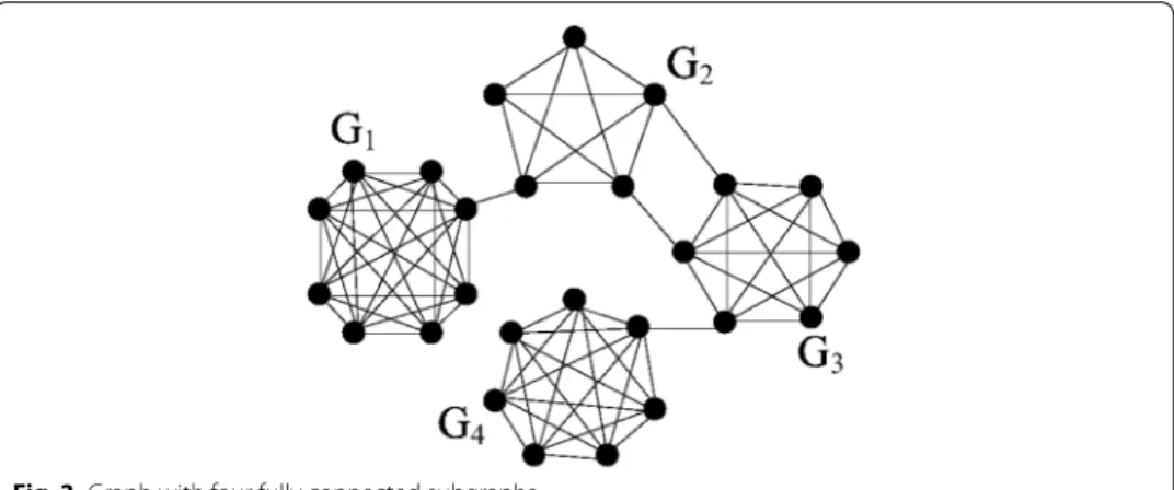
Example 2 Consider graph G = (N, E) , which consists of n = 26 nodes and m = 78
edges (see Fig. 3). This graph includes 4 fully connected subgraphs: G1 with 8 vertices N1 connected by 28 links, G2 with 5 vertices N2 connected by 10 links, G3 with 6 vertices N3 connected by 15 links, and G4 with 7 vertices N4 connected by 21 links. Subgraph G1 is connected with G2 by 1 edge, G2 with G3 by 2 edges, and G3 with G4 by 1 edge.
Firstly, calculate the potentials (7) for large-scale decompositions of G for any param-eter α ∈ [0, 1] . It is easy to check, that P(N) = 78 − 325α , P({N1, N2∪ N3∪ N4}) = 77− 181α , P({N1, N2∪ N3, N4}) = 76 − 104α , P({N1, N2, N3, N4}) = 74 − 74α.
Other coalition partitions give smaller potentials: P({N1∪ N2, N3∪ N4}) = 76 − 156α < 76− 104α , P({N1∪ N2∪ N3, N4}) = 77 − 192α < 77 − 181α , P({N1, N2, N3∪ N4}) = 75 − 116α < 76 − 104α , P({N1∪ N2, N3, N4}) = 75 − 114α < 76 − 104α.
We solve a sequence of linear inequalities in order to find maximum of the potential for all α ∈ [0, 1] . The result is presented in the table.
Nash-stable coalition partitions in Example 2
α Coalition partition Potential
[0, 1/144] N1∪ N2∪ N3∪ N4 78− 325α
[1/144, 1/77] N1, N2∪ N3∪ N4 77− 181α
[1/77, 1/15] N1, N2∪ N3, N4 76− 104α
[1/15, 1] N1, N2, N3, N4 74− 74α
Example 1 (ctnd) Note that for the unweighted version of the network example
presented in Fig. 1, there are only two stable partitions: = N for small values of α≤ 1/9 and = {{A, B, C}, {D, E, F}} for α > 1/9.
Another natural approach to define a symmetric value function is, roughly speak-ing, to compare the network under investigation with the configuration random graph model. The configuration random graph model can be viewed as a null model
for a network with no community structure. Namely, the following value function can be considered:
where Aij is the number of links between nodes i and j (multi-graph is allowed), di and dj are the degrees of nodes i and j, respectively, m = 1
2
l∈Ndl is the total number of links in the network, and βij = βji and δ are some parameters.
Note that if βij= β, ∀i, j ∈ N , and δ = 1 , the potential (7) coincides with the network modularity [15, 16]. If βij = β, ∀i, j ∈ N , and δ �= 1 , we obtain the generalized modularity presented first in [18]. The introduction of the non-homogeneous weights was proposed in [19] with the following particularly interesting choice:
The introduction of the resolution parameter δ allows one to obtain clustering with vary-ing granularity as well as to overcome the resolution limit [30].
Thus, we now have an interpretation based on coalition game of the modular-ity method. Namely, the coalition partition � = {S1, . . . , SK} which maximizes the modularity
gives the Nash-stable partition of the network in the hedonic game with the value func-tion defined by (8) with δ = 1 and βij= β.
Example 1 (ctnd) For the network example presented in Fig. 1, we
calcu-late P(N )= 3/2, P({B, C} ∪ {A, D} ∪ {E, F}) = P({A, B, C, D} ∪ {E, F}) = 7/2 and P({A, B, C} ∪ {D, E, F}) = 5 . Thus, according to the value function (8) with δ = 1 and βij = β (modularity value function), = {{A, B, C}, {D, E, F}} is the unique Nash-stable coalition partition.
The case of non-additively separable preferences
Now let us consider a few cases of non-additively separable preferences which still have potentials. First, we consider a slight modification of preference structure (6) which makes it non-additively separable. Namely, define the preference relation as follows:
where 1{·} is the indicator function, giving one if the argument is true, vij is defined as before in (6), and γ is a parameter representing the cost of coalition creation and allows us to control further the clustering resolution and granularity. As verified in the follow-ing proposition, in this case the game also has a potential.
(8) vij = βij Aij− δ didj 2m , βij = 2m didj . (9) P(�)= K k=1 i,j∈Sk,i�=j Aij− didj 2m (10) S1�iS2⇔ j∈S1 vij− γ 1{S1�= ∅} ≥ j∈S2 vij− γ 1{S2�= ∅},
Proposition 3 The hedonic clustering game defined by the preference relation (10) has
the following potential:
Proof Suppose that partition = {S1, ..., SK} maximizes the function (11), possibly locally. Then, if i moves from S�(i) to Sk , the value of (11) corresponding to the new par-tition ′ is different from the value corresponding to by
note that K is not changing. If i creates its own cluster, then the value of (11) correspond-ing to ′ is different from that for by
and in the case S�(i)= {i} , the difference is
If provides a maximum of (11), all these differences are negative. So, according to rela-tion (10), player i indeed has no incentive to move from her coalition S�(i) to another coalition and the function (11) can be interpreted as a potential.
Let us provide a few recommendations for the choice of α and γ . Similarly to [18], from the analysis of the mean field model corresponding to a stochastic block model (SBM), one can show that the value of α close to the link density ensures the internal stability of clusters in the mean field model of SBM. Thus, if a network has one main scale, such value of α gives good result. If a network has nested clustering structure, one can vary α to obtain clustering with the needed level of granularity. Again using the mean field model for SBM, one can show that the good value of γ corresponds to the product of α and the smallest size of the cluster we would like to obtain.
We mention that interestingly under a specific choice of parameters the globally optimal partition may contain disconnected clusters. However, such a choice of parameters is typi-cally not natural.
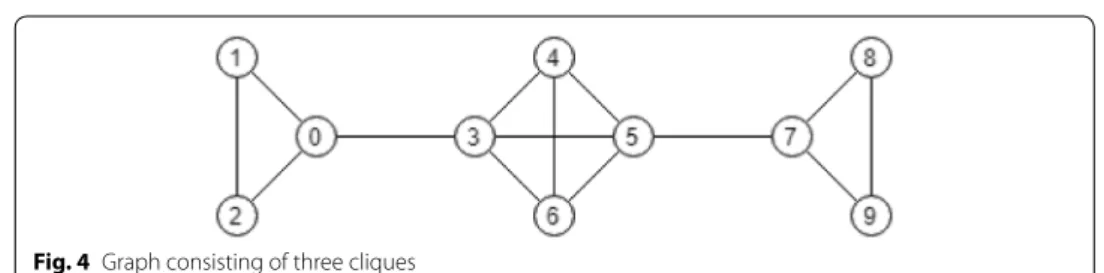
Example 3 Let us consider a graph that consists of a clique of four nodes and two
cliques of three nodes connected to it (see Fig. 4).
(11) Pα,γ(�)= K k=1 m(Sk)− α n(Sk)(n(Sk)− 1) 2 − γ K . j∈Sk vij− j∈S�(i) vij, −γ − j∈S�(i) vij, j∈Sk vij+ γ .
One can check that for α = 0.5 and γ = 5, the partitioning gives the maximum value to the potential Pα,γ( ˜�)= − 8.5 , while
An intuitive interpretation for this choice of parameters is that α is chosen significantly large to encourage splitting of clusters from the grand coalition and γ is also chosen sig-nificantly large to penalize the creation of independent clusters.
Next we would like to note that two well-known network partitioning methods: normal-ized cut [10, 33] and ratio cut [32] can also be viewed as particular instances of potential hedonic clustering games with non-additively separable preferences. Towards this end, let us introduce a few more definitions. Let S, T ⊂ N be two, possibly overlapping sets of nodes. Then, we define a cut W(S, T) as
Note that an edge is counted twice if its both ends lie in the same set. The volume of a set S∈ N is defined as the number of edges between its vertices
The normalized cut of a set S is defined by
where ¯S = N\S . If vol(S) = 0 , we define hNCUT(S)= +∞ . One can also define the ratio cut ˜ = {{0, 1, 2, 7, 8, 9}, {3, 4, 5, 6}} Pα,γ({{0, 1, 2, 3, 4, 5, 6, 7, 8, 9}}) = − 18.5, Pα,γ({{0, 1, 2, 3, 4, 5, 6}, {7, 8, 9}}) = − 9, Pα,γ({{0, 1, 2}, {3, 4, 5, 6}, {7, 8, 9}}) = − 9. W (S, T )= i∈S,j∈T 1{(i, j) ∈ E}. vol(S)= 1 2W (S, S). hNCUT(S)= W (S, ¯S) W (S, S) = 1 2 W (S, ¯S) vol(S) , hRCUT(S)= W (S, ¯S) |S| .
Similar to the normalized cut, we assign hRCUT(S)= +∞ , if |S| = 0 , i.e., S = ∅ . Then, the normalized cut [10, 33] and ratio cut [32] network partitioning methods are based on the following potentials
respectively. Similar to the proof of Proposition 3, one can check that the above poten-tials correspond to the following preferences: for the normalized cut
and the ratio cut
respectively. Thus, two more, well-known network partitioning methods can be cast into our general framework. A very important benefit of such interpretation is that in con-trast to the original formulations, we now do not require a priori knowledge of the num-ber of clusters.
Gibbs sampling approach for hedonic games with potential
We note that finding Nash equilibrium in a game with potential is equivalent to finding a maximum of the game’s potential. To find a maximum of the game’s potential, we can follow the approach based on Gibbs sampling. Let us consider the following Gibbsian distribution over all partitions:
It is easy to see that as β → ∞ , the distribution concentrates on the partition corre-sponding to the maximum of the potential P(�).
Next, denote by the set of indices of the network clusters and by �i→σ the (re)assign-ment of node i to cluster σ ∈ � and run the Glauber dynamics [18, 44] according to
(12) PNCUT(�)= − S∈� hNCUT(S), (13) PRCUT(�)= − S∈� hRCUT(S), (14) S1�iS2⇔ W (S1 {i}, ¯S1\{i}) vol(S1 {i}) − W (S1, ¯S1\{i}) vol(S1) ≤ W (S2 {i}, ¯S2\{i}) vol(S2 {i}) − W (S2, ¯S2\{i}) vol(S2) (15) S1�iS2⇔ W (S1 {i}, ¯S1\{i}) |S1| + 1 − W (S1, ¯S1\{i}) |S1| ≤ W (S2 {i}, ¯S2\{i}) |S2| + 1 − W (S2, ¯S2\{i}) |S2| , (16) ρ(�)= exp (βP(�)) ∀ ˜�exp βP( ˜�) . (17) P�→�′ = 1 n � i∈N exp (βP(�)) � s∈�exp (βP(�i→s)), if � ′= �, exp(βP(�′)) �
s∈�exp (βP(�i→s)), if �′= �i→σ,
that is, we choose randomly a node and reassign this node to a new cluster according to the conditional Gibbsian distribution (clearly, it can happen that the node remains in its current cluster). It is well known that the Glauber dynamics corresponds to the revers-ible Markov chain with the stationary distribution given by (16), see e.g., [44]. One can also cool down the temperature as in simulated annealing [45] in order to find the parti-tion with the global maximum of the potential. We define one iteraparti-tion as n updates of nodes according to (17). Typically and as will be demonstrated in the next section, if we take a reasonably high inverse temperature β , the process (17) often finds good-quality partition already after 5–10 iterations. The complexity of one iteration is very light in the case of sparse graphs, i.e., O(|E|).
A sample generated by the above-described Glauber dynamics appears to have signifi-cant variance. To reduce it, the generalized empirical covariance matrix of several sam-ples can be used, similar to [46] where the standard covariance matrix has been used for the case of two clusters. For one sample, the elements of the generalized covariance matrix are defined as follows:
The empirical generalized covariance matrix of a set of samples is the average of their generalized covariance matrices, i.e.,
An (i, j)th value of the generalized covariance matrix indicates how often the ith and
jth nodes appear in the same cluster.
Then, given a generalized covariance matrix one can extract the community structure using threshold-based or PCA-based methods.
Numerical validation
In this section, we validate the proposed approaches on synthetic and real-world net-works. As a benchmark, we take a widely used clustering method sklearn.clus-ter.spectralclustering from [47]. The method is based on the eigen elements of the normalized Laplacian and K-means postprocessing and have demonstrated good performance in many previous studies.
If it is available, the ground truth clustering is denoted by true and the clustering obtained by an algorithm as test . Each time we specify which algorithm we test against the ground truth. We measure the difference between these two partitions by the follow-ing function from [48]:
M(1)i,j = 1, if σ (i) = σ (j),−1, otherwise. .
ˆ M= 1 T T t=1 M(t). (18) E (�true, �test)= 1 −1
nπ:�truemax→�test
σ∈�true nσ,π(σ ).
Synthetic network: stochastic block model
We first evaluate various clustering algorithms based on potential hedonic games on sto-chastic block model (SBM), a synthetic network with known community structure. An SBM with | | clusters is represented by a symmetric square matrix P where pσ,σ is a den-sity of edges inside the cluster σ and pσ,σ′ = pσ′,σ is a density between clusters σ and σ′ . Specifically, we use SBM with two communities of 50 and 150 nodes, intra-cluster den-sity p11= p22= 0.1 and inter-cluster density p12= p21= 0.02 . We start from a random coloring and run the process for 100 iterations.
In Fig. 5, we show an example of the Glauber dynamics using NCUT potential (12). For small β = 10 we observe unstable behavior, while for large β = 500 the process evolves around a local maximum that provides relatively bad clustering (49 out of 50 nodes of the first community and only 116 out of 150 of the second community are clus-tered correctly).
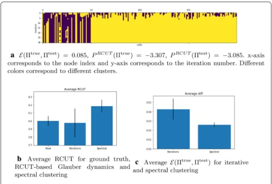
Now let us take a closer look at RCUT (13). We discovered that in our example the ground truth partition does not maximize the potential. The process converges fast to a clustering that differs from the ground truth and has larger PRCUT than the ground truth partition. We tested the algorithm on a set of 100 graph instances generated according to the SBM and we show the results in Fig. 6 where we also compare it to the spectral clustering from [47]. One can see that while the Glauber dynamics generally ends up with PRCUT(�test) >PRCUT(�true) . The spectral clustering procedure provides a solu-tion that has smaller PRCUT but is closer to the ground truth.
Next let us evaluate the performance of the clustering based on the potential Pα , see (7). Empty clusters do not cause any singularities in Pα unlike in PNCUT and PRCUT . Hence, the final partition can have less clusters than | | . Let us at first restrict the num-ber of clusters by setting = {0, 1} . In this context, we have two natural choices for ini-tial coloring of a graph: either, as before, we can choose colors uniformly at random, or we can assign same color to all nodes. We tested both settings on a set of 100 SBM graph instances. The best results are obtained with α = 0.05 and β = 10 . If we assign clusters at random at initialization, the process may not converge to a good coloring. Assigning the same initial color to all the nodes leads to better results. Fig. 7a and b shows evolu-tion on the same graph with different initial colorings. The average E after 20 iteraevolu-tions for random-cluster initialization is 0.033, for single-cluster initialization it is 0.006; while the standard spectral clustering, i.e., the continuous relaxation of the NCUT [33] pro-vides a result with average E(�true, �test)= 0.025 . We can conclude that the Pα-based clustering significantly outperforms the spectral clustering in terms of accuracy. How-ever, it depends on the parameter α that determines the penalty for large clusters. If α is too small, the uniform coloring becomes the ground state, as already indicated in Propo-sition 2. If α is too large, the obtained clusters will be relatively of the same size but may not represent the real community structure.
We can also try to detect the real number of clusters, if we choose large . Here we can test the case when initially all nodes receive different colors | | = |V | . We discovered that the final clustering consists of 9 or 10 clusters on average, most of which contain very few nodes. See Fig. 7c for an example of such clustering process.
To prevent the problem described in the previous paragraph, we modify Pα to Pα,γ , see Eq. (11), by introducing a penalty term proportional to the number of non-empty
clusters. The potential Pα,γ depends on parameters α and γ that determine penalties for disparate clusters and for the total number of them, respectively. We tested the respec-tive Glauber dynamics on the same set of random instances of SBM with parameters α= 0.05 , γ = 5 , β = 10 , and | | = |V | = 200 . We run the process for 20 iterations and averaged the coloring over the last 10 of them. We obtained the following results: 2 clus-ters were determined in every graph instance and the average E(�true, �test) is 0.0057. The average E(�true, �test) for the spectral clustering is 0.0252.
In order to validate further the method based on Pα,γ-potential, we tried it on dif-ferent sets of graphs of difdif-ferent clustering structures with the same algorithm param-eters α , γ , and β . On a set of 100 homogeneous Erdős–Rényi random graphs of 200 nodes with edge density 0.1, our algorithm ended up with a uniform coloring on 99 of them and on one graph it finished with 2 clusters where the smaller one contains only two nodes. Given a set of 100 graph instances of SBM with clusters of 50, 150, and 200 nodes, the algorithm correctly determined the number of clusters in each graph and provided on average E(�true, �test)= 0.006 , while spectral clustering provided on
Fig. 5 The iterations of NCUT-based Glauber dynamics for different β ; PNCUT
(�true)= − 1.40 . x-axis corresponds to the node index and y-axis corresponds to the iteration number. Different colors correspond to different clusters
average E(�true, �test)= 0.026 . On a set of 100 graph instances containing 4 clusters of 50, 100, 150, and 200 nodes, the algorithm after 20 iterations determined 4 clusters in 90 graphs and 3 clusters in 10 graphs. The average E(�true, �test) is 0.0335. However, if we increase the number of iterations to 50, we determine correctly 4 clusters for 95 graphs
Fig. 6 The iterations of RCUT-based Glauber dynamics for β = 200 and comparison to the ground truth and
spectral clustering
Fig. 7 The iterations of hedonic-based process for α = 0.05 and β = 10 for a graph with Pα(�true
)= − 785 .
x-axis corresponds to the node index and y-axis corresponds to the iteration number. Different colors
and 3 clusters for the others. The average E(�true, �test) becomes 0.0185. The average E (�true, �test) of the spectral clustering on the same set of graphs is 0.0375.
The above results can be further improved by using the generalized covariance matrix. The application of the generalized covariance matrix will be illustrated in some of the following network examples.
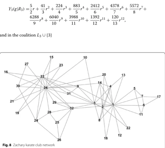
Real‑world network with ground truth: Karate club
Consider the popular example of the social network from Zachary karate club (see Fig. 8). In his study [49], Zachary observed 34 members of a karate club over a period of 2 years. Due to a disagreement developed between the administrator of the club and the club’s instructor there appeared two new clubs associated with the instructor (node 1) and administrator (node 34) of sizes 16 and 18, respectively.
The authors of [15] divide the network into two groups of roughly equal size using modularity and hierarchical clustering tree. They show that this split corresponds almost perfectly with the actual division of the club members following the break-up. Only one node, node 3, is classified incorrectly by the method of [15].
Let us first apply the Myerson value approach to the karate club network. To perform the analytic study, let us start from the ground truth partition [49]
By using subindex 3, we emphasize the importance of player 3. By enumerating all sim-ple paths and using formula (4), we find the Myerson value for player 3 in coalition R3
and in the coalition L3∪ {3}
R3= {1, 2, 3, 4, 5, 6, 7, 8, 11, 12, 13, 14, 17, 18, 20, 22} and L3= N \ R3. Y3(g|R3)= 5 2r+ 41 3 r 2 + 224 4 r 3 + 883 5 r 4 + 2412 6 r 5 + 4378 7 r 6 + 5572 8 r 7 + 6288 9 r 8 +604010 r9+3988 11 r 10 + 139212 r11+120 13r 12 ,
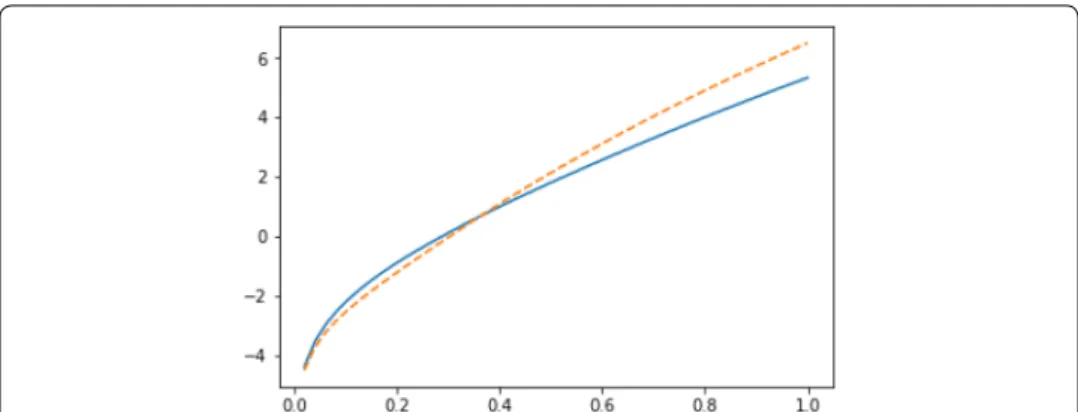
We have plotted both Y3(g|R3) and Y3(g|L3∪ {3}) as functions of r in Fig. 9. If r is smaller than 0.231, node 3 has no incentive to move from coalition R3 to coalition L3 . Recall that the modularity-based method of [15] would displace player 3 into the wrong coalition L3.
It is also interesting to investigate the imputations of the other two border nodes 9 and 10. If we plot the imputations for node 10: Y10(g|L3) and Y10(g|R3∪ {10}) (see Fig. 10), we observe that as for node 3, for smaller values of r (i.e., for r < 0.363 ), node 10 has no incentive to leave the coalition L3 ; whereas for the values of r greater than 0.363, node 10 has incentive to change the coalition.
As it is clear from Fig. 11, node 9 has no incentive to leave the coalition L3 with any value of r. Thus, we can conclude that the ground truth partition [49] is internally stable according to the Myerson value approach if r < 0.231 . This has a nice intuitive interpretation. Humans cannot count easily long paths and consequently one needs to apply heavy discounting to mimic humans’ decisions.
Let us now apply the hedonic game approach with Glauber dynamics to the karate club network. We started from a random partition into two clusters and run the algo-rithm using the potential (7) with α = 0.046 , which corresponds to 1/3 of the edge density, and β = 20 . The algorithm stabilizes after around 5 iterations and the mean error after 10 iterations in 100 runs was 20.0%, which roughly corresponds 7 misclas-sified nodes. However, the partitioning results differ significantly from run to run.
By applying the spectral clustering algorithm from [47] to Zachary karate club net-work, we obtain an average error of 25.8%.
To reduce the variance of the Glauber dynamics and hence the clustering error, we computed the empirical generalized covariance matrix ˆM for the results of 10
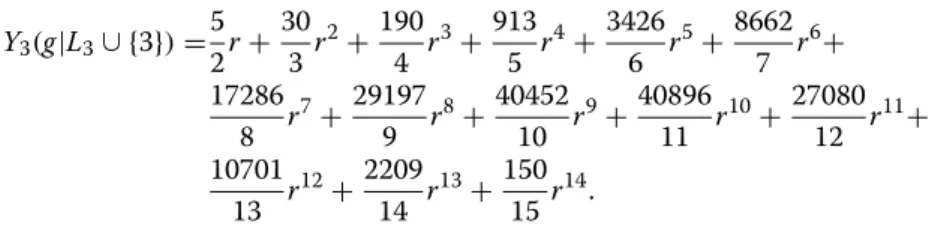
Y3(g|L3∪ {3}) = 5 2r+ 30 3 r 2 + 190 4 r 3 + 913 5 r 4 +3426 6 r 5 +8662 7 r 6 + 17286 8 r 7 + 29197 9 r 8 + 40452 10 r 9 +40896 11 r 10 +27080 12 r 11 + 10701 13 r 12 +2209 14 r 13 + 150 15 r 14 .
Fig. 9 Imputations for node 3 in Zachary karate club network: Y3(g|R3) (solid line) vs Y3(g|L3∪ {3}) (dashed
independent runs of 10 iterations of the Glauber dynamics and then extracted the community structure using the PCA algorithm. Only node 9 was misclassified, which is a border node.
The application of the generalized covariance matrix in addition to the Gibbs sam-pling really helps to consistently obtain high-quality results.
We would like to note that the application of the generalized covariance matrix to the spectral clustering method from [47] does not improve significantly its results since spectral clustering gives less noisy, however, more biased results compared to the hedonic game approach.
Real‑world network with ground truth: Dolphins
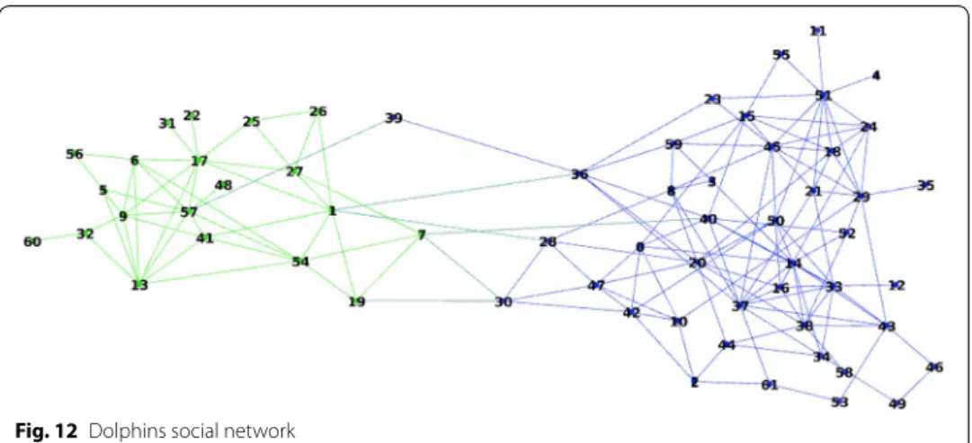
Consider now the Dolphins social network from [50]. This network presented in Fig. 12
was constructed from observations of a community of 62 bottle nose Dolphins over a period of 7 years from 1994 to 2001. The nodes in the network represent the Dolphins, and the ties between nodes represent the associations between dolphin pairs occurring more often than expected by chance.
Fig. 10 Imputations for node 10 in Zachary karate club network: Y10(g|L3) (solid line) vs Y10(g|R3∪ {10})
(dashed line) in semilog scale
Fig. 11 Imputations for node 9 in Zachary karate club network: Y9(g|L3) (solid line) vs Y9(g|R3∪ {9}) (dashed
The ground truth partition is presented by two coalitions: and
We studied the Dolphins network using the hedonic game approach with Glauber dynamics in a similar way as we did for Zachary karate club. Note that because of a very large number of simple paths in this network, the application of the Myerson value approach was not feasible. The following parameter values were used: α = 0.028 , which corresponds to 1/3 of the edge density, and β = 20 . The algorithm stabilizes after around 10 iterations and the mean error after 20 iterations in 100 runs was 24.8%. As with Zach-ary karate club, the partitioning results differ significantly from run to run.
By applying the spectral clustering algorithm from [47], we obtain an average error of 7.5%.
We computed the empirical generalized covariance matrix ˆM of the results of 10 inde-pendent runs of 20 iterations of the Glauber dynamics and then extracted the commu-nity structure using the PCA algorithm. Then, only one node, node 39, was misclassified. This is a border node connected to only two nodes of different clusters.
In contrast, computing the covariance matrix of 10 results of independent runs of spectral clustering algorithm from [47] led to 4 misclassified nodes: 22, 31, 48, 60.
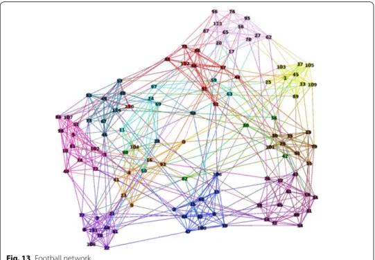
Real‑world network with many clusters and ground truth: Football
The American College Football network [15] represents the games between Division IA Colleges during the regular fall 2000 season (see Fig. 13).
The nodes in the network represent the teams and the links are the games between the teams. There are 115 teams and each team belongs to one of the 12 conferences. The communities in the network are the conferences. So, the ground truth partition is given by 12 coalitions:
L= {1, 5, 6, 7, 9, 13, 17, 19, 22, 25, 26, 27, 31, 32, 41, 48, 54, 56, 57, 60}
R = {0, 2, 3, 4, 8, 10, 11, 12, 14, 15, 16, 18, 20, 21, 23, 24, 28, 29, 30, 33, 34, 35, 36, 37, 38, 39, 40, 42, 43, 44, 45, 46, 47, 49, 50, 51, 52, 53, 55, 58, 59, 61}.
As was the case of the Dolphins network, we could not apply the Myerson value approach to the football network because of the difficulty in enumerating all simple paths. In contrast, the hedonic game approach can easily be applied.
One of the main advantages of the hedonic game approach with Pα,γ potential (11) is the fact that it does not require the number of clusters as a parameter. Let us test on the football network, which consists of 12 clusters, how the hedonic game approach with Pα,γ potential can perform without a priori knowledge of the number of clusters.
We set the following parameters of the potential: α = 0.093 (edge density), γ = 10 . We run the Glauber dynamics with random initial partition into 20 clusters and the inverse noise β = 10 for 20 iterations. The clustering dynamics stabilizes after around 10 iterations. We performed 50 independent runs. The average number of detected clusters was 10.22 and the average percentage of misclassified nodes is 13.5%.
As with Zachary and Dolphins networks, we computed the empirical generalized covariance matrix of the clustering results. Since our goal was to determine the clus-ters without providing its number to the algorithm, we used a simple threshold-based clustering algorithm instead of the PCA algorithm: we build a weighted graph using the generalized covariance matrix as its adjacency matrix and removed the edges with
C1 = [112, 48, 92, 44, 75, 66, 91, 86, 57, 110]; C2 = [50, 24, 69, 11, 97, 59, 63]; C3 = [80, 82, 42, 36, 90]; C4 = [45, 109, 37, 25, 1, 33, 103, 105, 89]; C5 = [9, 4, 104, 0, 93, 16, 41, 23]; C6 = [5, 74, 3, 98, 10, 40, 84, 81, 52, 102, 107, 72]; C7 = [68, 108, 78, 77, 8, 51, 21, 22, 7, 111]; C8 = [32, 6, 13, 47, 39, 100, 15, 106, 64, 60, 2]; C9 = [61, 99, 43, 14, 12, 31, 38, 18, 54, 34, 71, 26, 85]; C10 = [29, 19, 94, 35, 55, 30, 101, 79]; C11 = [46, 67, 73, 83, 114, 88, 53, 49, 58, 28]; C12 = [62, 65, 95, 17, 70, 56, 113, 27, 87, 20, 76, 96].
weights below 0.5; the connected components of the resulting graph indicate clusters in the original network.
The resulting graph contained 13 connected components, i.e., we identified 13 clus-ters in the initial network that is quite close to the ground truth value 12. The percent-age of the misclassified nodes is 6.9%, which signifies that the generalized covariance matrix improved significantly the quality of the clustering results.
Large real‑world network without ground truth: Co‑authorships in Math‑Net.ru
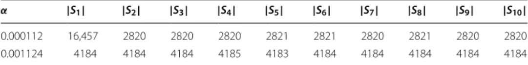
To test scalability and efficiency of the hedonic game approach, we have chosen to cluster a fairly large social network. We have crawled the site Math-Net.ru, Russian Mathematical Portal, for the co-authorship graph [51]. We further extracted the giant connected component of this co-authorship network, which includes 41,840 authors. We have applied the hedonic game with the potential (7) and run the modified Glau-ber dynamics using round robin node schedule with random permutation. Twenty iterations of the modified Glauber dynamics run for about 2 min on Intel Core Duo 1.6 GHz processor and 5GB RAM. We have initialized process with a single cluster and restricted the number of clusters to ten. We have again observed stabilization of the modified Glauber dynamics at 15–20 iterations. Recall that one iteration of the modified Glauber dynamics requires O(|E|) operations, which is quite a reasonable cost in the case of sparse networks and which is the case of most real-world networks. We have chosen significantly high value of β , which corresponds to nearly greedy algorithm. First, we have run the modified Glauber dynamics with α corresponding to the average edge density. This has lead to unbalanced clusters, see Table 1. By expect-ing clusters, we have observed that nearly all academicians (aka leaders of scientific schools) have been clustered to one largest cluster. However, when we have increased α tenfold, the clustering became much more balanced and the academicians have been distributed more evenly among the clusters.
Large synthetic SBM network with ground truth
To continue testing scalability and efficiency of the hedonic game approach and in particular to confirm a rapid convergence of the Glauber dynamics to a good solution, we consider a large stochastic block model graph with known communities. Specifi-cally, we have generated an SBM with two clusters of sizes 50,000 and 150,000 nodes. We have generated the intra-cluster links with probability 0.0002 and the inter-clus-ter links with probability 0.00005. We run the Glauber dynamics associated with the potential (7), setting α = 0.0001 and β = 10 . In a typical run, after 7 iterations, only 97 nodes from the smaller cluster were misclassified to the larger cluster and only 65 nodes from the larger cluster were misclassified to the smaller cluster. It is not
Table 1 Cluster sizes in Math-Net.ru
α |S1| |S2| |S3| |S4| |S5| |S6| |S7| |S8| |S9| |S10|
0.000112 16,457 2820 2820 2820 2821 2821 2820 2821 2820 2820
surprising that by the “gravity” effect the larger cluster attracted more nodes. We find that 7 iterations of the Glauber dynamics are not at all a large cost for partitioning 200,000 node network.
Conclusion and future research
We have presented two cooperative game theory-based approaches for network parti-tioning. The first approach is based on the Myerson value for graph constrained coop-erative game, whereas the second approach is based on hedonic games which explain coalition formation. We find the second approach especially interesting as it gives a very natural way to tune the clustering resolution and generalizes the modularity, ratio cut, and normalized cut-based approaches. Within the hedonic games framework, we have proposed two new methods which particularly well regularize clustering resolu-tion and help to adjust the level of granularity. We have shown that normalized cut and ratio cut methods can be modified to avoid the requirement of the number of clusters. All approaches that can be represented as hedonic games with potentials can be very efficiently implemented using Gibbs sampling with Glauber dynamics and generalized covariance matrix. The application of the generalized covariance matrix significantly improves the quality and stability of the clustering results. Our research plans are to test and to compare our methods on more social networks and to study analytically the con-vergence rate of Gibbs sampling.
Authors’ contributions
The contribution of all four authors to the manuscript is quite balanced. All authors read and approved the final manuscript.
Author details
1 Inria Sophia Antipolis, 2004 Route des Lucioles, 06902 Valbonne, France. 2 Higher School of Economics, 16 Soyuza
Pechatnikov St., St. Petersburg 190121, Russia. 3 Institute of Applied Mathematical Research, Karelian Research Center,
Russian Academy of Sciences, 11 Pushkinskaya St., Petrozavodsk 185910, Russia. 4 Saint-Petersburg State University, 7/9
Universitetskaya Nab., St. Petersburg 199034, Russia. Acknowledgements
We would like to thank the editor and the referees for very useful remarks and suggestions that helped to significantly improve the presentation of the results. The work of the first and fourth authors is partly supported by the joint labora-tory Inria—Nokia Bell Labs, the joint Inria-UFRJ team THANES and by UCA-JEDI Idex Grant “HGAPHS.” The second and the third authors are supported by Russian Fund for Basic Research (Projects 16-51-55006, 16-01-00183). The third author is supported by Russian Science Foundation (Project 17-11-01709).
Competing interests
The authors declare that they have no competing interests. Publisher’s Note
Springer Nature remains neutral with regard to jurisdictional claims in published maps and institutional affiliations. Received: 31 October 2017 Accepted: 11 October 2018
References
1. Abbe E. Community detection and stochastic block models: recent developments. J Mach Learn Res. 2018;18(177):1–86.
2. Fortunato S. Community detection in graphs. Phys Rep. 2010;486(3):75–174.
3. Fortunato S, Hric D. Community detection in networks: a user guide. Phys Rep. 2016;659:1–44.
4. Jonnalagadda A, Kuppusamy L. A survey on game theoretic models for community detection in social networks. Soc Netw Anal Mining. 2016;6(1):83.
6. Schaeffer SE. Graph clustering. Comput Sci Rev. 2007;1(1):27–64.
7. Avrachenkov K, Dobrynin,V, Nemirovsky D, Pham SK, Smirnova E. Pagerank based clustering of hypertext document collections. In: Proceedings of the 31st annual international ACM SIGIR conference on research and development in information retrieval, SIGIR 2008, Singapore, July 20–24; 2008, p. 873–4.
8. Avrachenkov K, Chamie ME, Neglia G. Graph clustering based on mixing time of random walks. In: IEEE international conference on communications, ICC 2014, Sydney, Australia, June 10–14. 2014. p. 4089–94.
9. Dongen S. Performance criteria for graph clustering and Markov cluster experiments. Amsterdam: CWI (Centre for Mathematics and Computer Science); 2000.
10. Meilă M, Shi J. A random walks view of spectral segmentation. In: The 8th international workshop on artifical intel-ligence and statistics (AISTATS). 2001.
11. Newman ME. A measure of betweenness centrality based on random walks. Soc Netw. 2005;27(1):39–54. 12. Pons P, Latapy M. Computing communities in large networks using random walks. ISCIS. 2005;3733:284–93. 13. Blatt M, Wiseman S, Domany E. Clustering data through an analogy to the potts model. In: Advances in neural
information processing systems 8, NIPS, Denver, CO, Nov 27–30. 1995. p. 416–22.
14. Blondel VD, Guillaume J-L, Lambiotte R, Lefebvre E. Fast unfolding of communities in large networks. J Stat Mech. 2008;10:10008.
15. Girvan M, Newman ME. Community structure in social and biological networks. Proc Natl Acad Sci. 2002;99(12):7821–6.
16. Newman ME. Modularity and community structure in networks. Proc Natl Acad Sci. 2006;103(23):8577–82. 17. Raghavan UN, Albert R, Kumara S. Near linear time algorithm to detect community structures in large-scale
net-works. Phys Rev E. 2007;76(3):036106.
18. Reichardt J, Bornholdt S. Statistical mechanics of community detection. Phys Rev E. 2006;74(1):016110. 19. Waltman L, van Eck NJ, Noyons EC. A unified approach to mapping and clustering of bibliometric networks. J
Inform. 2010;4(4):629–35.
20. McSweeney PJ, Mehrotra K, Oh JC. A game theoretic framework for community detection. In: International confer-ence on advances in social networks analysis and mining, ASONAM 2012, Istanbul, Turkey, 26–29 August 2012. p. 227–34.
21. Mazalov VV, Trukhina LI. Generating functions and the myerson vector in communication networks. Discrete Math Appl. 2014;24(5):295–303.
22. Mazalov VV, Avrachenkov K, Trukhina L, Tsynguev BT. Game-theoretic centrality measures for weighted graphs. Fund Inform. 2016;145(3):341–58.
23. Gomez D, González-Arangüena E, Manuel C, Owen G, del Pozo M, Tejada J. Centrality and power in social networks: a game theoretic approach. Math Soc Sci. 2003;46(1):27–54.
24. Suri NR, Narahari Y. Determining the top-k nodes in social networks using the shapley value. In: Proceedings of the 7th international joint conference on autonomous agents and multiagent systems. International foundation for autonomous agents and multiagent systems, Vol. 3, p. 1509–12.
25. Szczepański PL, Michalak T, Rahwan T. A new approach to betweenness centrality based on the shapley value. In: Proceedings of the 11th international conference on autonomous agents and multiagent systems, Vol 1, p. 239–46. 26. Michalak TP, Aadithya KV, Szczepanski PL, Ravindran B, Jennings NR. Efficient computation of the shapley value for
game-theoretic network centrality. J Artif Intell Res. 2013;46:607–50.
27. Chen W, Teng S-H. Interplay between social influence and network centrality: a comparative study on shapley centrality and single-node-influence centrality. In: Proceedings of the 26th international conference on World Wide Web. International World Wide Web Conferences Steering Committee. 2017. pp. 967–6.
28. Skibski O, Michalak TP, Rahwan T. Axiomatic characterization of game-theoretic centrality. J Artif Intell Res. 2018;62:33–68.
29. Bogomolnaia A, Jackson MO. The stability of hedonic coalition structures. Games Econ Behav. 2002;38(2):201–30. 30. Fortunato S, Barthélemy M. Resolution limit in community detection. Proc Natl Acad Sci. 2007;104(1):36–41. 31. Leskovec J, Lang KJ, Dasgupta A, Mahoney MW. Community structure in large networks: natural cluster sizes and
the absence of large well-defined clusters. Internet Math. 2009;6(1):29–123.
32. Hagen L, Kahng AB. New spectral methods for ratio cut partitioning and clustering. IEEE Trans Comput Aided Design Integ Circuits Syst. 1992;11(9):1074–85.
33. Shi J, Malik J. Normalized cuts and image segmentation. IEEE Trans Pattern Anal Mach Intell. 2000;22(8):888–905. 34. Zhou L, Cheng C, Lü K, Chen H. Using coalitional games to detect communities in social networks. In: International
conference on web-age information management. Berlin: Springer; 2013. p. 326–31.
35. Zhou L, Lü K, Cheng C, Chen H. A game theory based approach for community detection in social networks. In: Proceedings Big Data—29th British national conference on databases, BNCOD 2013, Oxford, UK, July 8–10. 2013. p. 268–81.
36. Basu S, Maulik U. Community detection based on strong nash stable graph partition. Soci Netw Anal Mining. 2015;5(1):61.
37. Avrachenkov KE, Kondratev AY, Mazalov VV. Cooperative game theory approaches for network partitioning. In: International computing and combinatorics conference (COCOON/CSoNet). Berlin: Springer; 2017. p. 591–602. 38. Myerson RB. Game Theory. Cambridge: Harvard University Press; 2013.
39. Peleg B, Sudhölter P. Introduction to the theory of cooperative games, vol. 34. Berlin: Springer; 2007. 40. Mazalov V. Mathematical game theory and applications. New York: Wiley; 2014.
41. Myerson RB. Graphs and cooperation in games. Math Operat Res. 1977;2(3):225–9. 42. Jackson MO. Allocation rules for network games. Games Econ Behav. 2005;51(1):128–54. 43. Jackson MO. Social and economic networks. Princeton: Princeton University Press; 2010.
44. Levin DA, Peres Y, Wilmer EL. Markov chains and mixing times. Rhode Island: American Mathematical Soc., Provi-dence; 2009.
45. Hajek B. Cooling schedules for optimal annealing. Math Operat Res. 1988;13(2):311–29. 46. Berthet Q, Rigollet P, Srivastava P. Exact recovery in the ising blockmodel. Ann Stat. 2018;41:1780.
47. Pedregosa F, Varoquaux G, Gramfort A, Michel V, Thirion B, Grisel O, Blondel M, Prettenhofer P, Weiss R, Dubourg V, Vanderplas J, Passos A, Cournapeau D, Brucher M, Perrot M, Duchesnay E. Scikit-learn: machine learning in python. J Mach Learn Res. 2011;12:2825–30.
48. Meilă M, Heckerman D. An experimental comparison of model-based clustering methods. Mach Learn. 2001;42(1–2):9–29.
49. Zachary WW. An information flow model for conflict and fission in small groups. J Anthropol Res. 1977;33(4):452–73. 50. Lusseau D, Schneider K, Boisseau OJ, Haase P, Slooten E, Dawson SM. The bottlenose dolphin community of
doubt-ful sound features a large proportion of long-lasting associations. Behav Ecol Sociobiol. 2003;54(4):396–405. 51. Zhizhchenko AB, Izaak AD. The information system Math-Net.Ru. Application of contemporary technologies in the