Optimizing jobs timeouts on clusters and production grids

HAL Id: hal-00691828

https://hal.archives-ouvertes.fr/hal-00691828

HAL is a multi-disciplinary open access archive for the deposit and dissemination of sci-entific research documents, whether they are pub-lished or not. The documents may come from teaching and research institutions in France or abroad, or from public or private research centers.

L’archive ouverte pluridisciplinaire HAL, est destinée au dépôt et à la diffusion de documents scientifiques de niveau recherche, publiés ou non, émanant des établissements d’enseignement et de recherche français ou étrangers, des laboratoires publics ou privés.

Optimizing jobs timeouts on clusters and production

grids

Tristan Glatard, Johan Montagnat, Xavier Pennec

To cite this version:

Tristan Glatard, Johan Montagnat, Xavier Pennec. Optimizing jobs timeouts on clusters and produc-tion grids. 2006, pp.23. �hal-00691828�

LABORATOIRE

INFORMATIQUE, SIGNAUX ET SYSTÈMES DE SOPHIA ANTIPOLIS

UMR 6070

O

PTIMIZING JOBS TIMEOUTS ON CLUSTERS AND

PRODUCTION GRIDS

Tristan Glatard, Johan Montagnat, Xavier Pennec

Projet

RAINBOW

Rapport de recherche

ISRN I3S/RR–2006-35–FR

N

ovembre 2006

LABORATOIREI3S: Les Algorithmes / Euclide B – 2000 route des Lucioles – B.P. 121 – 06903 Sophia-Antipolis Cedex, France – Tél. (33) 492 942 701 – Télécopie : (33) 492 942 898

RÉSUMÉ:

Ce document présente une méthode pour optimiser la valeur du délai d’expiration (timeout) de tâches de calcul sur une grille. Il est fondé sur un modèle du temps d’exécution des tâches qui considère que la latence du système de gestion de tâches de la grille est une variable aléatoire. Le modèle prend aussi en compte un taux de panne pour modéliser soit des grappes fiables soit des grilles de production qui sont caractérisées par leur pannes. Les systèmes de gestion de tâches sont d’abord étudiés en considérant des distributions classiques de la latence. Plusieurs comportements surviennent en fonction du poids de la queue de la distribution de la latence et de la proportion de pannes. Nous présentons ensuite des résultats expérimentaux fondés sur des mesures de la distribution de la latence et du taux de panne sur la grille de production EGEE. Ces résultats montrent qu’utiliser la valeur optimale du délai d’expiration fournie par notre méthode réduit l’impact des pannes et peut conduire à une accélération de 1.36 sur des systèmes fiables.

MOTS CLÉS:

délai d’expiration, grilles de production, latence, variabilité

ABSTRACT:

This paper presents a method to optimize the timeout value of grid computing jobs. It relies on a model of the job execution time that considers the job management system latency through a random variable. It also takes into account a proportion of outliers to model either reliable clusters or production grids characterized by faults causing jobs loss. Job management systems are first studied considering classical distributions of the latency. Different behaviors are exhibited, depending on the weight of the tail of the distribution and on the amount of outliers. Experimental results are then shown based on the latency distribution and outlier ratios measured on the EGEE grid infrastructure. Those results show that using the optimal timeout value provided by our method reduces the impact of outliers and leads to a 1.36 speed-up for reliable systems without outliers.

KEY WORDS:

Optimizing jobs timeouts on clusters and production grids

Tristan Glatard

, Johan Montagnat

1

_{I3S, CNRS, UNSA}

{glatard,johan}@i3s.unice.fr

Xavier Pennec

_{INRIA, Asclepios}

Xavier.Pennec@sophia.inria.fr

Abstract

This paper presents a method to optimize the timeout value of computing jobs. It relies on a model of the job execution time that considers the job management system latency through a random variable. It also takes into account a proportion of outliers to model either reliable clusters or production grids characterized by faults causing jobs loss. Job management systems are first studied considering classical distributions. Different behaviors are exhibited, depending on the weight of the tail of the distribution and on the amount of outliers. Experimental results are then shown based on the latency distribution and outlier ratios measured on the EGEE grid infrastructure1_{. Those results show that using the optimal} timeout value provided by our method reduces the impact of outliers and leads to a 1.36 speed-up even for reliable systems without outliers.

1 Introduction

A growing number of distributed applications is relying on large scale workload management sys-tems. These applications usually trigger hundreds, thousands or even more jobs. Although large scale systems provide very high throughput as a direct consequence of the huge amount of resources avail-able, they also introduce high and variable latencies that drastically degrade the performances of the application competing with other users’ computations. The latency corresponds to the duration between the submission date and the one at which the job execution effectively starts. It includes the submission, scheduling and queuing times but also data transfers and delays in the monitoring system. Furthermore, less reliable systems such as production grids are also impacted by outliers.

The variability impacts jobs latency in a normal operation mode. It mainly comes from the hetero-geneity of the infrastructure (endogen hardware and software factors) and from the load imposed to it (exogen factor). In this document, we will model the system latency by a probabilistic distribution.

Outliers correspond to system faults that lead to huge latencies prevailing on the ones of the other tasks of the application. Those latency values can be considered as infinite.

Typical faults generating outliers are hardware failures, locally heavy load or scheduling errors leading to a job being queued in a extremely long queue. This outlier mode can be quantified by its proportion of jobs that never return.

1_{http://www.eu-egee.org/}

Both variability and outliers penalize applications that rely on the completion of a high number of jobs. Indeed, a single job is then able to slow down the whole application. In case where there are dependencies between the jobs (e.g. in case of application workflows), the effects of variability and outliers are even more critical and lead to accumulated performance drops.

From the user point of view, strategies to reduce the impact of variability and outliers include multi-submission [1] (a given job is submitted many times and only the first completion is considered), jobs grouping (many jobs are grouped together to reduce the number of submissions) [2,3] and timeouting [4,

5]. Multi-submission is an aggressive strategy and job grouping is not always possible. Timeouting and resubmitting abnormally long jobs is a common strategy. Choosing the timeout value is often let to the administrator or the end user. However, a non trivial trade off has to be found as a too long timeout will penalize the jobs completion time too much, while a too short one may be overkilling, causing the unnecessary resubmission of jobs that almost completed. Hence, timeout strategies have been designed in areas as different as TCP throughput optimization [6], HTTP requests [7,8] or power saving devices [9].

To propose a timeout optimization, we first model jobs execution time in section2. We then present in section3some results of timeout optimization on classical distributions. To show how the optimization behaves on a real infrastructure, we are particularly interested in the asymptotic behavior of the system and on the impact of outliers. We finally present in section4some experimental results from a distribu-tion of the latency measured on the EGEE producdistribu-tion grid. To facilitate legibility, many of the proofs of the theoretical results are deferred in appendix.

2 Model of the job execution time

We adopted a probabilistic modeling of the large-scale workload manager. This approach has already been successfully reported to tackle related scheduling problems [11,12]. We will denote random vari-ables with capital letters whereas fixed values will be lowercase. For a random variable V, fVdenotes it

probability density function (pdf) and FV denotes its cumulative density function (cdf).

Let J be the total duration of a job (including all its potential resubmissions) and t_∞be a user defined timeout value. The system is seen as a black box introducing a positive latency R on the job wall-clock time r in case of normal operation. The outlier ratio is denoted ρ. r is assumed to be a fixed value depending only on the job nature whereas R is a random variable.

We denote with q the probability for a job to timeout. A job timeouts either if it is an outlier or if it faces a latency which is superior to t_∞. Thus:

q = ρ + (1 − ρ)P(r + R>t∞)

and then, q = 1 − (1 − ρ)FR(t∞− r). (1) If the job timeouts, it is canceled and resubmitted. We neglect the cost of canceling and resubmitting a job as well as the resulting overload on the system, so that consecutive submissions are considered as independent. Let Ji be the duration of the job from its ith submission to its completion. Ji can be

recursively defined as:

Ji=

! r + R with probability 1 − q

t∞+Ji+1 with probability q. (2)

For the sake of clarity, we will assume that r = 0. This hypothesis is not restrictive. In the rest of the equations, it corresponds to the variable change u = t − r. In case of real job executions, r would have to

be added to the timeout value. The goal is to express J = J1(through its cdf FJ) with respect to R and

t∞. J can only be superior to nt∞if the job timed-out n times. Thus:

P(J > nt∞) = qn so that P(J < nt∞) = 1 − qn. (3) We have the value of FJ(x) = P(J < x) for every x = nt∞. We now have to obtain a complete expression of FJ. Interpolating FJin every [nt∞,(n + 1)t∞] is clearly not suitable. Indeed, those intervals can be quite large with respect to the job execution time and the error coming from the interpolation is likely to produce inconsistent results. We can notice that FJ(t) represents the probability for J to be

inferior to t, so that for all t in [nt∞,(n + 1)t∞[:

FJ(t) = P(J < t|t ∈ [nt∞,(n + 1)t∞])

= P(J < nt∞) + P(nt∞<J < t | t ≤ (n + 1)t∞) and thus, according to equation3:

FJ(t) = 1 − qn+P(nt∞< J < t | t ≤ (n + 1)t∞). (4) Given that t ≤ (n + 1)t∞, a job duration J can only be in [nt∞,t] if the job timed-out n times (probability

qn_{) and if it succeeded on the (n + 1)}th_{attempt i.e. it was not an outlier (probability 1 − ρ) and R ≤ t − nt} ∞ (probability FR(t − nt∞)). Therefore, P(nt∞ < J < t | t ≤ (n + 1)t∞) = qn(1 − ρ)FR(t − nt∞). We finally get, ∀t ∈ [nt∞,(n + 1)t∞[:

FJ(t) = 1 − qn+qn(1 − ρ)FR(t − nt∞). (5) Given that R>0, FJ(0) = 0 and lim∞FJ = 1. Moreover, FJ is continuous at every nt∞. Indeed, according to equation5, the expression of FJat the lower bound of the segment [nt∞,(n + 1)t∞] is:

FJ(nt∞) = 1 − qn+qn(1 − ρ)FR(0) = 1 − qn

Moreover, at the upper bound of this segment, FJ is:

FJ((n + 1)t∞) = 1 − qn+qn(1 − ρ)FR((n + 1)t∞− nt∞) = _{1 − q}n+qn(1 − ρ)FR(t∞)

= _{1 − q}n+qn(1 − q) (given equation1with r = 0) = _{1 − q}n+1

However, in general, FJis not differentiable in nt∞, ∀n. Note that if ρ = 0, then equation5resumes to:

FJ(t) = 1 − qn+qnFR(t − nt∞) with q = 1 − FR(t∞). Thus, taking outliers into account corresponds to multiplying FRby the (1 − ρ) factor.

2.1 Illustration for ρ =0

If no outlier are present, the choice of a timeout value can be evaluated by comparing FR and FJ.

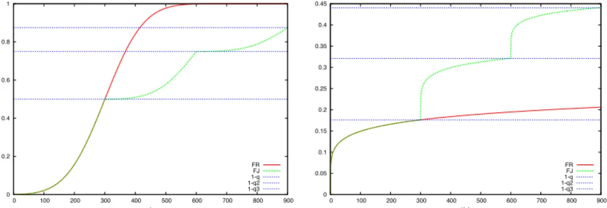
Figure 1 displays an example of cdf for R (plain red curve) and J (dashed green curve). Notice the singularities at nt_∞ points. On top, the distribution of R is Gaussian with a mean 300 seconds and standard deviation 100 seconds, truncated above zero to avoid negative latency times. The timeout value is equal to the mean of the original Gaussian (300 seconds). It is of course a very low timeout value leading to many resubmissions. We can graphically notice that for every t, FR(t) > FJ(t), which means

that for every time value t, there is a higher probability that R < t than that J < t. In this case, it would thus have been better not to set any timeout value as it highly penalizes the execution.

On the other hand, the bottom of figure1displays an example of cdf of R and J in a case where the timeout choice improves the execution. The timeout value is still 300 seconds but the law of R has a longer tail than in the former example. R is actually log-normal, with µ=15 seconds and σ=10 seconds. In this case, it seems that for every t, FR(t) < FJ(t), which means that the timeout improves the execution

time in this case.

0 0.2 0.4 0.6 0.8 1 0 100 200 300 400 500 600 700 800 900 t FR FJ 1-q 1-q2 1-q3 0 0.05 0.1 0.15 0.2 0.25 0.3 0.35 0.4 0.45 0 100 200 300 400 500 600 700 800 900 t(s) FR FJ 1-q 1-q2 1-q3

Figure 1. Example of cdf of R and J. Left: bad timeout choice. Right: good timeout choice.

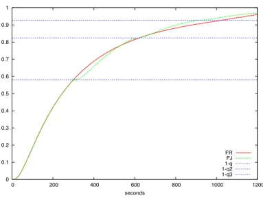
As suggested by those graphical remarks, the impact of some timeout choices on the job execution time may be evaluated only by comparing FJ and FR. However, apart from those particular cases, it is

often not possible to have general results on the comparison between FJand FRat every time point t and

the configuration displayed on figure2is observed. On this figure, the distribution of R is log-normal, with µ = 5.5s, σ = 1s and a timeout value of 300s. In this case, minimizing the expectation of J with respect to t_∞is a natural solution to optimize the timeout value.

2.2 Expectation of J

Computing the expectation of a job execution time, general conclusion can be made on its behavior when the timeout value increases, independently from the system latency distribution. As shown in appendixA, the expectation of J is:

EJ(t∞)= 1 FR(t∞) " t_∞ 0 u fR(u)du + t_∞ (1 − ρ)FR(t∞)− t∞ . (6)

0 0.1 0.2 0.3 0.4 0.5 0.6 0.7 0.8 0.9 1 0 200 400 600 800 1000 1200 seconds FR FJ 1-q 1-q2 1-q3

Figure 2. No general result onFJ.

Equation6compares to similar expressions derived for modeling completion times probabilistically : equation 6 in [5] and equation 1 in [4]. In both cases, the authors introduced a fixed cost penalty to resubmission that we consider to be zero (there is almost no overhead induced by job resubmission on a large scale system). In [5], the authors also derives higher moments of J and some relevant properties about them (e.g. their existence). Our hypotheses are similar to theirs except that they do not take into account outliers that are of major importance on the infrastructures we are targeting. As stated above, this parameter is characteristic of unreliable systems and they are needed to properly model a grid infrastructure. In [4], the authors do take into account the outlier ratio (denoted L). However, the studied hypotheses do not really match ours : the case of a client being unable to hold more than one connection (so-called simple client) is not developed, even if noticeable remarks (such as the fact that the timeout values of all the resubmissions have to be identical) are done.

As shown in in appendixB, EJhas the following limits:

lim t∞→∞ EJ(t∞) = +∞ if ρ ! 0 (7) and lim t∞→∞ EJ(t∞) = ER otherwise. (8)

If ρ ! 0, the line ER+_1−ρρ t∞is an asymptote of EJ(t∞).

The first limit can be explained by noticing that a single outlier may lead to an infinite execution time. When t∞→ +∞, the probability for encountering an outlier tends towards 1 and the expected execution time tends towards infinity. The second limit is also intuitive: in absence of outliers, if no timeout value is set, then the system latency would not be disturbed and the expectation of a job duration would resume to the one of the system latency.

Equations7and8show that ρ as a major impact on the system behavior. The case ρ = 0 corresponds to a reliable cluster management system: faults causing jobs loss are very unlikely (highly reliable LAN, robust schedulers). The case ρ > 0 is needed to model grid infrastructures. Lower reliability of WANs, scale effects and less mature workload management middlewares lead to a significant number of outliers.

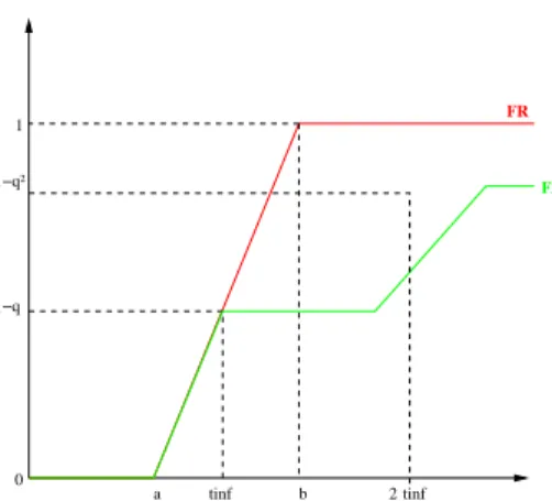
1 0 a b 1−q FJ FR 1−q² tinf 2tinf

Figure 3. Behavior ofFJfor a uniform distribution without outliers.

For instance on the EGEE infrastructure, ρ is in the order of 2%. In case of outliers it is mandatory to set a timeout value.

3 Results on classical distributions

In this section, we study some classical distributions from a theoretical point of view in order to understand how the timeout value impacts the expectation of the job duration both with and without outliers. We explore distributions with light tails (uniform, truncated Gaussian and Weibull with shape parameter >1), heavy tails (Weibull with shape parameter <1 and log-normal) and power tails (Pareto) to show how they exhibit different behavior. The exponential and Weibull distributions will constitute a transition between light and heavy-tailed distributions. The Weibull one is indeed light-tailed for a shape parameter greater than 1 and heavy-tailed otherwise. Light-tailed distributions are the ones that decay faster than the exponential. In this case, there exists a such that: lim_t→+∞eat_{(1 − F(t)) = 0. On}

the contrary, heavy-tailed distributions decay more slowly than the exponential : lim_t→+∞eat_{(1 − F(t)) =}

+∞. Power-tailed distributions are a subset of the heavy-tailed ones. In this case, there exists a and b such that limt→+∞1−F(t)ta =b.

For each distribution, our goal is to determine the optimal timeout value ˆt∞ = arg mint∞{EJ(t∞)}. In

case of very reliable systems (when no outliers are present), the optimal value of the timeout may be +∞, which means that no timeout should be set. Another singular optimal timeout value is 0. This configuration occurs when the probability for the job to face a null latency is so high that it is interesting to resubmit the job as soon as one knows that it is going to face a non null latency. This later result would only be realistic if it was possible to resubmit an arbitrarily large number of jobs at no additional cost. Obviously, the overhead induced on any real system would finally slow down the process.

3.1 Uniform distribution

In this case, the pdf of the system latency is:

fR(t) =

! ₁

b−a if t ∈ [a, b]

a+b 2 a b timeout value EJ a+b 2 a+b 2 +b ρ 1−ρ a b timeout value EJ

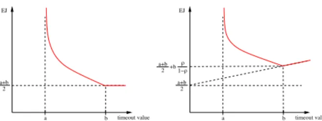
Figure 4. Behavior ofEJ(t∞)for the uniform distribution without (left) and with (right) outliers.

We can derive from equation6the expectation of J:

EJ(t∞) =                      +∞ if t∞≤ a t_∞+a 2 +t∞ b−t∞+ρ(t∞−a) (t∞−a)(1−ρ) if t∞∈ [a, b] b+a 2 +t∞ ρ 1−ρ otherwise. (10)

The shape of EJ(t∞) is depicted on figure 4. The optimal timeout value is b both with and without outliers. Even without outliers, setting the timeout to +∞ is optimal because the expectation of J is constant in [b,+∞[.

If there is no outliers, it can be graphically noticed that setting a timeout always penalizes the execu-tion. Indeed, as figure3shows, we have FJ(t) ≤ FR(t), for every timeout value t∞and every time point t.

3.2 Truncated Gaussian

Normal distributions are the most commonly used but they do not exclude negative values. In our case, the latency cannot be lower than 0. We are thus considering Gaussian distributions with mean µ and standard-deviation σ truncated above 0. The pdf and cdf of the system latency are:

fR(t) =        1 Φ(µ_σ) 1 √ 2πσe −12(t−µσ) 2 if t ≥ 0 0 otherwise, FR(t) = Φ(µ σ)−Φ( µ−t σ) Φ(µ σ) with Φ(t) = √1 2π 't −∞e −12u2du.

As shown in appendixE, the expectation of the job duration is then:

µ + σφ (_µ σ ) − φ(µ−t∞ σ ) Φ(_σµ)_{− Φ}(µ−t∞ σ )+ 1 1 − ρt∞         Φ(µ−t∞ σ ) Φ(_σµ)_{− Φ}(µ−t∞ σ )+ρ         . with φ = Φ)_.

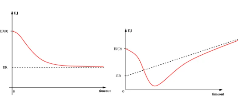
The curve of EJ is plotted on figure5. EJ exhibits different behaviors depending on the presence of

outliers or not. If there are no outliers (ρ = 0), EJ is decreasing towards its limit ERwhen t∞→ +∞. On the other hand, when ρ ! 0, then EJexhibits a global minimum reached for ˆt∞< + ∞. The corresponding

0 timeout EJ EJ(0) ER EJ EJ(0) timeout 0 ER

Figure 5. Behavior of the expectation of J for a truncated Gaussian distribution without (left) and with (right) outliers.

proof is based on the fact that the forth derivative of EJ is always positive, so that we can study the

existence of a root in the lower order derivatives. It is reported in appendixF.

If the distribution of the system latency is Gaussian and ρ = 0, timeouting is not a solution to limit the impact of variability, regardless of the variability order of magnitude. In this case, other solutions such as multi-submissions or job grouping have to be studied.

3.3 Exponential distribution

In this case, the cdf of the system latency is:

FR(t) = 1 − e−αt.

And according to equation6, the expectation of J is:

EJ(t∞) = 1 α +

ρt∞

(1 − ρ) (1 − e−αt∞).

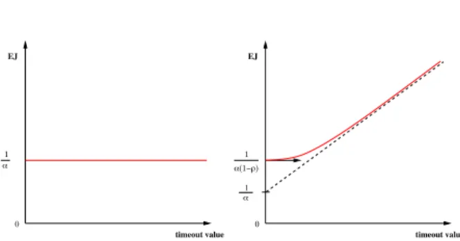
The curve of EJ(t∞) is depicted on figure 6. In case of outliers, EJ is thus increasing and the best

timeout value is ˆt∞ =0. If there are no outliers, the expectation of J is independent from t∞, which is a singular behavior particular to the exponential distribution, as proved in appendixC. This characteristic of the exponential distribution has to be related to the fact that this distribution is the only one to be memory-less. In this case, at a given instant, knowing that a job is still in the system does not give any information about its future behavior and the timeout value thus does not impact the distribution of J. The exponential distribution is a particular case of the Weibull one which is studied in the next section.

3.4 Weibull distribution

The Weibull distribution is typically used to model the failure of technical devices. For this distribu-tion, the cdf of the grid latency is:

FR(t) = 1 − e−(

t

λ)

k

k is a shape parameter and λ is a scale parameter of the distribution. In the context of failure modeling,

timeout value 0 EJ 1 α α(1−ρ) 1 1 α timeout value 0 EJ

Figure 6. Behavior ofEJ for an exponential distribution without (left) and with (right) outliers.

time and k>1 means that the failure rate increases over time. In our situation, the random variable R can be seen as the date at which a job completes, i.e R models the success of a job. Note that the exponential distribution of parameter 1/λ is a Weibull distribution with k=1.

In this case, we have the following results for timeout optimization, in absence of outliers:

• If k > 1, then setting a timeout value always penalizes the execution, whatever this value is. The optimal timeout value is thus +∞ (no timeout).

• If k < 1, then the timeout value has to be as low as possible. The optimal timeout value is 0. • If k = 1, then the distribution of R is exponential and the timeout value does not impact the job

execution time.

The corresponding proofs are reported in appendix D. They are based on a comparison between FJ and

FR, following the remarks done in section2.1.

The obtained results are coherent with the classical interpretation of the shape parameter of the Weibull distribution. Indeed, when k>1, the success rate of a job is increasing over time, which ex-plains that timeouting will penalize the job. On the contrary, when k<1, the success rate of a job is then decreasing over time, and timeouting as soon as possible becomes mandatory.

When outliers are present, we conjecture that the behaviour remains the same when the shape pa-rameter is lower than 1. Indeed, outliers lengthen the tail of the distribution and thus lower the timeout value. Similarly, when the shape parameter is greater that 1, it seems that the expectation of the job execution time with respect to the timeout value reaches a global finite minimum. Its derivative tends towards minus infinity (it seems to be equivalent to − λk(k−1)

(1−ρ)tk−1

∞ ) when the timeout value tends towards zero

and EJ is thus decreasing on an intervall starting from t∞ = 0. As it is tending towards +∞ when t∞ tends towards +∞, it has to reach a global finite minimum. However, this behaviour is still not proved.

3.5 Log-normal distribution

The log-normal distribution is a typical example of heavy-tailed distribution. In this section, we assume that R has a log-normal distribution with parameters µ and σ. In this case, the cdf and pdf of the system latency are respectively:

FR(t) = Φ0 ln t − µ σ 1 and fR(t) = 1 t√2πσe −(ln t−µ)2_{2σ2 .}

The expectation and standard-deviation of R are: ER=eµ+ σ2 2 and σ R= ( eσ2 − 1)e2µ+σ2 . (11)

In this case, as reported in appendixG, we can show that EJis:

ER. 0 Φ (x_{∞− σ)} Φ(x∞) +eσx∞−σ22 0 1 (1 − ρ)Φ(x∞)− 1 11 (12) where x∞= ln(t_∞) − µ σ

This expression shows that the minimization of EJcan be performed independently from µ on the

trans-formed variable x_∞. The obtained solution ˆx_∞(σ, ρ) only depends on σ and ρ. The optimal timeout value can then be written as:

ˆt_∞(µ, σ) = eµ_{K(σ, ρ) where K(σ, ρ) = e}σˆx∞(σ,ρ) ₍₁₃₎ and: ˆx_∞(σ, ρ) = arg minx∞ 0 Φ (x_{∞− σ)} Φ(x∞) + eσx∞−σ22 0 1 (1 − ρ)Φ(x∞)− 1 11 .

K(σ, ρ) is actually the optimal timeout value for µ = 0.

We also have the following limit for t∞=0: lim

t_∞→0EJ(t∞) = x∞lim→−∞

EJ(x∞) = +∞.

This infinite limit proves that when ρ ! 0, there exists a finite non null optimal timeout value that minimizes EJ. Indeed, in this case, the limit of EJ when t∞tends towards infinity is infinite, according to equation7and EJthus has to reach a global minimum.

The existence of a global minimum of EJ(t∞) when ρ ! 0 is not straight-forward. Given the infinite limit of EJ when t∞ tends towards 0 and given that EJ(+∞) = ER, it resumes to the existence of a t∞ for which EJ(t∞)<ER. If σ > 1, then t∞ = eµ satisfies this relation. Indeed, in this case, x∞ = 0 and according to equation 12, EJ(x∞ = 0) = ER(2Φ(−σ) + e−

σ2

2 ). A numeric resolution then shows that

EJ<ERif and only if σ ! 0.9311. Numeric simulations also suggest that EJhas a global minimum even

for lower values of σ. However, an analytic proof still has to be done.

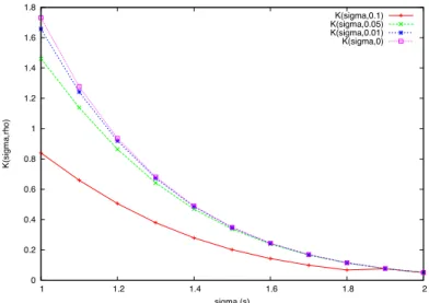
Figure7displays a simulation of the optimal timeout value for µ=0, several values of the outlier ratio and σ ranging from 1 to 2. We first can notice that K(σ, ρ) seems decreasing with respect to ρ. The timeout value thus has to be reduced when the proportion of outliers is increasing, which is coherent. Moreover, given an outlier ratio, the optimal timeout value for µ = 0 is decreasing as σ is growing. It is also coherent because the standard-deviation of the log-normal distribution is increasing with respect to σ (see equation 11). The optimal timeout value thus has to be reduced as the variability of the infrastructure is growing.

0 0.2 0.4 0.6 0.8 1 1.2 1.4 1.6 1.8 1 1.2 1.4 1.6 1.8 2 K(sigma,rho) sigma (s) K(sigma,0.1) K(sigma,0.05) K(sigma,0.01) K(sigma,0)

Figure 7. Evolution of the optimal timeout value forµ=0 in the log-normal case.

3.6 Pareto distribution

The Pareto distribution was introduced to represent the distribution of wealth and proved to be very accurate to model a large class of computer systems measurements (jobs durations, size of the files, data transfers length on the Internet. . . ) [13,14]. It is an example of power tailed distribution. The cdf of the system latency is then:

FR(t) = 1 −

2 a

a + t

3ν

with a and ν > 0.

The expectation is only defined for ν>1. Then:

ER =

a v − 1.

In this case, the expression of EJcan be directly derived from equation6and it is:

a + t∞ν − a (_a+t ∞ a )ν (1 − ν)4(a+t∞ a )ν − 15 + t∞ (1 − ρ)4(a+t∞ a )ν − 15 + ρ 1 − ρt∞.

We also have the following limit when the timeout value is null:

lim

t∞→0

EJ(t∞) =

a v(1 − ρ).

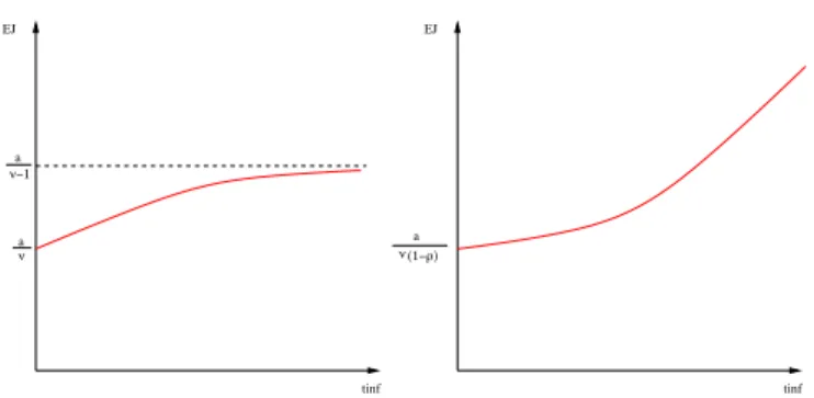
We then can show (see proof in appendixH) that the expectation of the job duration time is increasing with respect to the timeout value, regardless of the ρ value. The optimal timeout value is thus 0. The behavior of EJ(t∞) is depicted on figure8.

a ν ν−1 a tinf EJ tinf EJ ν (1−ρ) a

Figure 8. Behavior ofEJfor a Pareto distribution ofR. Left: no outliers ; Right:ρ !0.

Distribution Without outliers (ρ = 0) With outliers (ρ>0)

Uniform +∞ (or b) b Truncated Gaussian +∞ 0 < ˆt∞< +∞ Weibull k>1 +∞ 0 < ˆt∞< +∞ Exponential any 0 Weibull k<1 0 0 Log-normal (µ,σ) ˆt_∞=eµ_{K(σ) < +∞ 0 < ˆt} ∞< +∞ Pareto (ν>1) 0 0

Table 1. Optimal timeout values for the studied distributions ofR.

3.7 Results summary and interpretation

Table1displays a summary of the results we obtained for various distributions of the system latency. Those results suggest that the weight of the tail of the distribution of the system latency is a discrimi-natory parameter for the timeout optimization when outliers are not present. Indeed, only heavy-tailed distributions such as the log-normal, or the Pareto ones lead to finite optimal timeout values. In this case, the optimization speeds the execution up. On the other hand, when the distribution of the system latency decays more rapidly than the exponential, then setting a timeout value always penalizes the execution and the optimal timeout is +∞. The exponential distribution stands in the middle and is not affected by the timeout value.

As noticed in section2, taking into account the outliers resumes to multiplying FRby the factor (1-ρ).

In this case, the distribution of the system latency becomes heavy-tailed as lim_x→+∞eax_{(1 − (1 − ρ)F} R(x)) =

+∞ when a > 0. Effectively, in this case, the optimal timeout value that we found is always finite, which is coherent with this interpretation.

Results for the Weibull distribution with outliers and for the log-normal one without outliers and with σ<0.94 are only conjectures.

3.8 Performance improvement

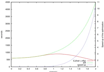
In case of reliable systems (without outliers), the expectation of the job duration without timeout equals to the one of the system latency. In this case, the ratio ER

0 500 1000 1500 2000 2500 3000 3500 4000 4500 0 0.2 0.4 0.6 0.8 1 1.2 1.4 1.6 1.8 2 1 2 3 4 5 6 7 8 9 10 11 seconds

Speed-up of the optimization

sigma(s)

EJ(hat t_infty) ER speed-up

Figure 9. Evolution of the speed-up of the optimization forµ =6.4sin the log-normal case.

optimization. If the latency of the system is light-tailed, then setting a timeout value always penalizes the execution. The best strategy is thus to set the timeout value to infinity. In this case, the optimization does not provide any speed-up with respect to the expectation of the system latency. Concerning the limit case of an exponential distribution, the expectation of the job duration is independent from the timeout value and the optimization does not lead to any speed-up.

The optimization becomes interesting for heavy-tailed distributions as already suggested. For the log-normal case, figure 9displays a numerical simulation of the evolution of the speed-up of the optimization with respect to σ for a particular value of µ. We can see that the speed-up is growing with σ. The higher the system latency, the more interesting the timeout optimization. Concerning the Pareto distribution, the optimized expectation of the job duration without outliers is a_ν, whereas the one obtained without setting any timeout is ER = _ν−1a . The speed-up obtained by the optimization is thus _ν−1ν . This value is

maximal for ν = 1 and decreases towards 1 when ν increases. Under Pareto assumption, the variance of the system latency( νa2

(ν−2)(ν−1)2

)

is decreasing with respect to ν. Here again, the more variable the latency of the infrastructure, the more important the speed-up yielded by the optimization.

When outliers are present, the optimization of the timeout prevents the expectation of J to be infinite. The impact of the optimization can then be evaluated by comparing the optimized expectation of the job duration to the one obtained without outliers. In case of a uniform distribution, outliers add the term

b_1−ρρ to the expectation of the job duration. This term is increasing with respect to the outlier ratio and tends towards infinity when ρ tends towards 1. The exponential distribution and the Pareto one exhibit a similar behavior: the outliers introduce an extra 1

1−ρ factor on the expectation of the job duration. Here again, this factor tends towards infinity when the outlier ratio tends towards 1.

4 Experiments

In this section, we present experimental results obtained by measuring the distribution of the latency of the EGEE grid infrastructure on a particular time period. The EGEE grid is a pool of thousands

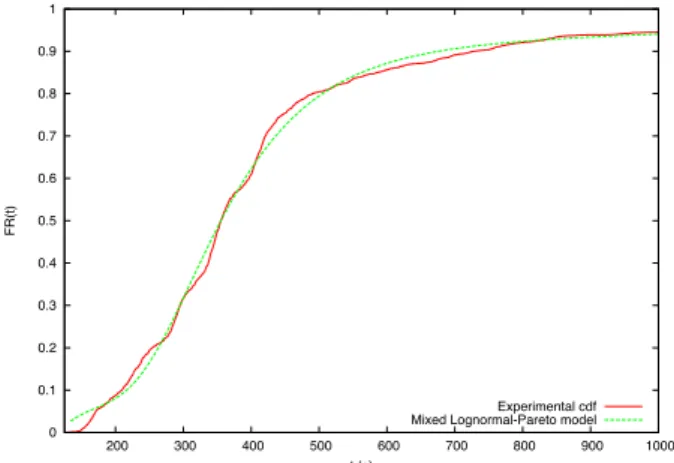
0 0.1 0.2 0.3 0.4 0.5 0.6 0.7 0.8 0.9 1 200 300 400 500 600 700 800 900 1000 FR(t) t (s) Experimental cdf Mixed Lognormal-Pareto model

Figure 10. Measured data (green) and best fitting Log-normal-Pareto model (red).

computers (standard PCs) and storage resources accessible through the gLite middleware. The resources are operated in computing centers, each of them running its internal batch scheduler. Jobs are submitted from a user interface to a central Resource Broker (RB) which dispatches them to the computing centers. EGEE is a production infrastructure with more than 25000 CPUs spread in more than 190 computing centers. It is characterized by its high throughput but also by its high latency, high variability and outliers. It is thus an ideal target to test our optimization procedure.

4.1 Measure of the distribution

To measure the distribution of the system latency on the EGEE grid, we submitted probe jobs that only consist in the execution of a /bin/hostname and we measure their round-trip time. We maintain a constant number of probes inside the system by submitting a new one as soon as one completed to avoid introducing any extra variability.

To measure the proportion of outliers, we consider a long duration T beyond which jobs are considered as outliers. When the value of T is sufficiently high, the measured outlier ratio, computed as the number of outliers jobs divided by the number of submitted ones is assumed not to depend on T and we use it as an approximation of the true one. However, by definition, outliers are rare phenomena, and the measure of the outlier ratio does not rely on a significant number of events. It is thus likely to be misestimated. Specific statistical methods concerning rare events [15] may be used to have a more precise estimation of the outlier ratio.

Our measure of the distribution of R gathers 2137 probe jobs spread on 3 different days and involving 3 RB. The maximal duration of those jobs was fixed to tmax = 10000 seconds. Beyond this value, we consider the job as an outlier. Given those conditions, we obtained an outlier ratio of 2.5 %. In normal operating mode, the measured distribution of R is plotted in green on figure10. It has an expectation of 393 seconds and a standard deviation of 792 seconds.

250 300 350 400 450 500 550 600 650 1000 2000 3000 4000 5000 6000 7000 8000 9000 10000 Expectation of J (s) timeout value (s) EJ in normal mode EJ with outliers asymtptot ER

Figure 11. Evolution of the expectation of J in the experimental case.

4.2 Timeout optimization

If we do not take outliers into account, the evolution of EJwith respect to the timeout value is plotted

in red on figure11. EJ then converges towards ERas predicted by the theoretical analysis. In this case,

EJ reaches a minimum for ˆt∞ =360s. At this optimal point, ˆEJ(ˆt∞) = 289s. The speed-up w.r.t to an execution without timeout is 1.36.

The evolution of EJ(t∞) taking the outliers into account is plotted in green on figure11. EJeffectively

tends to its asymptote. The optimal timeout value ˆt∞is now 358 seconds and ˆEJ(ˆt∞) has grown to 300 seconds. Setting the optimal timeout value thus limits the impact of the outliers to a 11-seconds loss, whereas it would be highly superior if the timeout value is not properly set, as suggested by figure11.

4.3 Model of the measured distribution

To relate those experimental results to the ones presented in the previous section, we here model the experimental distribution of the grid latency. The experimental data shown on figure 10cannot be rea-sonably fitted with any of the standard distributions described in section3. However, the distribution appears to be close to a log-normal distribution for low values (up to 500 seconds) and a Pareto distri-bution beyond. Based on this observation we fitted the experimental data with the following distridistri-bution which is an interpolation of the log-normal and Pareto ones, for t in [tmin,tmax]:

Fm R(t) = (1 − α(t)) Φ 0 ln(t − tmin) − µ σ 1 + (14) α(t)21 −2_{a + t}a 3 ν3 with α(t) = 0 t − tmin tmax− tmin 1k .

tmin denotes the smallest latency measured among the data (the cdf is zero below this value) and tmax the highest one. There are thus five parameters fully describing this model (µ, σ, a, ν, and k). α(t) is a weight function designed so that α(tmin) = 0 and α(tmax) = 1. The model thus tends to a log-normal distribution in tminand to a Pareto one in tmax.

We have estimated the best fit of the model14 with the experimental data by minimizing the least square criterion: arg min (µ,σ,a,ν,k)        tmax 6 i=tmin ( FmodelR (i) − F exp R (i) )2       

where Fexp_R (i) is the value of the measured distribution at time i. The optimal model is displayed on figure 10 (red curve). A Kolmogorov-Smirnov test was made to evaluate the quality of the model. When considering an undersampling of up to 1000 measurements, the Kolmogorov-Smirnov test value is D1000 = 1.35 (we used Dn = √n sup |FexpR − FmR|), which correspond to a p-value p = 0.051. The

tests is thus positive. It shows that a simple model (5 parameters) can accurately model the distribution measured over a very complex workload system (EGEE grid infrastructure) even when considering a very large data sample.

5 Conclusion

In this work, we presented a model of the job execution time taking into account the timeout value and resubmissions. We used it to optimize the timeout value of the jobs and we studied the optimization results for various latency distributions. Two cases have been distinguished, given that we consider that the job management system is prone to face outliers (grid) or not (cluster).

We showed that the optimal timeout value is highly dependent on the nature of the distribution of the system latency. In absence of outliers, the heavy-tailed distribution studied (log-normal) leads to a finite optimal timeout value whereas for the light-tailed ones (truncated Gaussian, uniform), setting a timeout value always penalizes the execution.

If we take outliers into account, our model predicts that the expectation of the job execution time is then diverging to +∞ when the timeout value tends towards +∞ for every distribution. The expectation of J has an asymptote whose slope only depends on the outlier ratio. The optimal timeout value is then finite for all the studied distributions, which can be explained by noticing that taking outliers into account lengthens the tail of the distribution.

We finally presented some experimental results from a distribution that was measured on the EGEE production grid. Results showed that even without outliers, a 1.36 speed-up can be achieved by using the optimal timeout value. Considering outliers, using the optimal timeout value is even more critical and the resulting optimal expectation of the job duration is close to the one obtained in absence of outliers.

However, some problems still remain to be able to use this optimization in practice. The most impor-tant one is to be able to dynamically measure the distribution of the non-stationary grid latency.

Acknowledgments

We thank Pierre Bernhard and Philippe Nain for useful advises. This work is partially funded by the French research program “ACI-Masse de donn´ees” (http://acimd.labri.fr/), AGIR project (http://www.aci-agir.org/). We are grateful to the EGEE European project for providing the grid infrastructure and user assistance.

References

[1] H. Casanova, “On the Harmfulness of Redundant Batch Requests,” in 15th IEEE International Symposium on High Performance Distributed Computing (HPDC’06), (Paris, France), pp. 255–266, June 2006.

[2] T. Glatard, D. Emsellem, and J. Montagnat, “Generic web service wrapper for efficient embedding of legacy codes in service-based workflows,” in Grid-Enabling Legacy Applications and Supporting End Users Work-shop (GELA’06), (Paris, France), June 2006.

[3] T. Glatard, J. Montagnat, and X. Pennec, “Probabilistic and dynamic optimization of job partitioning on a grid infrastructure,” in Parallel, Distributed and network-based Processing (PDP06), (Montb´eliard-Sochaux, France), pp. 231–238, Feb. 2006.

[4] L. Libman and A. Orda, “Optimal Retrial and Timeout Strategies for Accessing Network Resources,” IEEE/ACM Transactions on Networking (TN), vol. 10, pp. 551–564, Aug. 2002.

[5] A. van Moorsel and K. Wolter, “Analysis of Restart Mechanisms in Software Systems,” IEEE Trans. on Software Eng. (TSE), vol. 32, pp. 547–558, Aug. 2006.

[6] A. Kesselman and Y. Mansour, “Optimizing TCP Retransmission Timeout,” in International Conference on Networking, vol. 3421 of LNCS, (Saint-Denis de la R´eunion), Springer, Apr. 2005.

[7] P. Reinecke, A. van Moorsel, and K. Wolter, “A Measurement Study of the Interplay between Application Level Restart and Transport Protocol,” in Intl Service Availability Symposium (ISAS), vol. 3335 of LNCS, (Munich, Germany), pp. 86–100, May 2004.

[8] W. Xie, H. Sun, Y. Cao, and K. Trivedi, “Optimal Webserver Session Timeout Settings for Web Users,” in Computer Measurement Group Conference (CMGC), (Reno, NV, USA), pp. 799–820, Dec. 2002.

[9] P. Rong and M. Pedram, “Determining the optimal timeout values for a power-managed system based on the theory of Markovian processes: offline and online algorithms,” in Design, Automation and Test in Europe, (Munich, Germany), pp. 1128–1133, Mar. 2006.

[10] T. Glatard, J. Montagnat, and X. Pennec, “Optimizing jobs timeouts on clusters and production grids,” Tech.

Rep. I3S/RR-2006-35-FR,http://www.i3s.unice.fr/∼glatard/RR06.35.pdf, I3S, 2006.

[11] H. Gautama and A. J. C. van Gemund, “Symbolic Performance Estimation Of Speculative Parallel Pro-grams,” Parallel Processing Letters, vol. 13, no. 4, pp. 513–524, 2003.

[12] J. Schopf and F. Berman, “Stochastic Scheduling,” in Supercomputing (SC’99), (Portland, USA), 1999. [13] M. Harchol-Balter, “Task Assignment with Unknown Duration,” Journal of the ACM (JACM), vol. 49,

pp. 260–288, Mar. 2002.

[14] N. Ben Azzouna, Etude des m´ethodes d’´echantillonnage des flux pour la mesure dans les r´eseaux large bande. PhD thesis, Universit´e Pierre et Marie Curie - Paris VI, Paris, Sept. 2004.

[15] B. Beauzamy, M´ethodes probabilistes pour l’´etude des ph´enom`enes r´eels. Soci´et´e de Calcul Math´ematique S. A., Mar. 2004.

[16] T. Glatard, J. Montagnat, and X. Pennec, “Efficient services composition for grid-enabled data-intensive applications,” in IEEE International Symposium on High Performance Distributed Computing (HPDC’06), (Paris, France), June 2006.

A Expectation of J in the general case

B Limits of E

C Distributions for which the timeout value does not impact E

when ρ = 0

Let F be the cdf of a distribution which has this property. Then: ∀n ∈ N, ∀t∞∈ R+, 1 − (1 − F(t∞))n+(1 − F(t∞))nF(t − nt∞) = F(t) ⇒ ∀n ∈ N, ∀t∞∈ R+, G(t_∞)n_{G(t − nt} ∞) = G(t) with G = 1 − F ⇒ ∀n ∈ N, ∀t∞∈ R+, nH(t_∞) + H(t − nt∞) = H(t) with H = ln (G) ⇒ ∀n ∈ N, ∀t∞∈ R + , H)_{(t − nt} ∞) = H)(t)

H’ is thus periodic, with period nt_∞for every t_∞and every n. It is thus constant and we have H)_{(t) = α.} Thus, H(t) = αt +β. We thus have F(t) = 1−eβ_eαt_{. Moreover, the limit of F(t) has to be 1 when t → +∞,}

so that α<0 and β = 0, which demonstrates that the distribution of R has to be exponential.

D Behavior of E

in the Weibull case without outliers

We have: ∀n ∈ N, ∀t ∈ [nt∞,(n + 1)t∞], FJ(t) = 1 − qn+qnFR(t − nt∞) = _{1 − e}−n(t∞λ) k +e−n(t∞λ) k2 1 − e−(t−nt∞λ ) k3 = _{1 − e}− 2 n(t∞_λ)k+(t−nt∞ λ ) k3

We are going to compare FJ and FR. To do that, we will actually compare ln

( ₁ 1−FJ

)

and ln(_1−F1_R). The comparison resumes to study the sign of the following function ft_∞,n, for every n and every t∞ ( ft∞,n=ln ( ₁ 1−FJ ) − ln(_1−F1_R)): ∀n ∈ N, ∀t∞>0, ft_∞,n: [nt∞,(n + 1)t∞] → R t ,→ n2t∞ λ 3k + 2t − nt ∞ λ 3k − 2t λ 3k

If ft∞,nis positive, then setting a timeout improves the execution. The derivative of ft∞,nwith respect to t

is: f) t∞,n(t) = k λ 2₍ t−nt∞ λ )k−1 −(λt )k−13 . If k > 1: ft∞,n(nt∞) = (_t∞ λ )k( n − nk) <_{0 and ∀t ∈ [nt∞},(n + 1)t_∞], f) t∞,n(t) < 0. ft∞,n(t) is thus negative

on this interval and we have:

ln 0 1 1 − FJ(t) 1 − ln 0 1 1 − FR(t) 1 < 0 thus, FJ(t) < FR(t)

It proves that every timeout value penalizes the execution. The timeout thus has to be infinite.

If k < 1: ft∞,n(nt∞) = (_t ∞ λ )k( n − nk) >_{0 and ∀t ∈ [nt∞},(n + 1)t_∞], f) t∞,n(t) > 0. ft∞,n(t) is thus positive

on this interval and we have:

∀t > 0, ∀t∞>0, ln 0 1 1 − FJ(t) 1 − ln 0 1 1 − FR(t) 1 > 0 thus, FJ(t) > FR(t) Moreover, n(t∞ λ )k +(t−nt∞ λ )k

is decreasing with respect to t∞. Thus, ∀t∞>0, ∀t)∞>t∞, FJ,t)

∞(t) < FJ,t∞(t)

for every t. The optimal timeout value is thus 0.

E Expression of E

(t

) in the truncated Gaussian case

According to equation6, EJ(t∞) = 1 FR(t∞) " t_∞ 0 u fR(u)du + t_∞ (1 − ρ)FR(t∞)− t∞ = 1 Φ(µ_σ)_{− Φ}(µ−t∞ σ ) 1 √ 2πσ " t_∞ 0 ue−1 2(u−µσ) 2 du + t∞Φ (_µ σ ) (1 − ρ)(Φ(_σµ)_{− Φ}(µ−t∞ σ ))− t∞ Moreover, " t_∞ 0 ue−1 2(u−µσ) 2 du = σ2 " t∞−µ_σ −µσ ve(−1 2v2)dv + σµ " t∞−µ_σ −µσ e(−1 2v2)dv =σ2√2π 2 φ 2_µ σ 3 − φ 2_{µ − t∞} σ 33 +σµ√2π 2 Φ 2_µ σ 3 − Φ 2_{µ − t∞} σ 33 Thus, EJ(t∞) = µ + σ φ(_σµ)− φ(µ−t∞ σ ) Φ(_σµ)_{− Φ}(µ−t∞ σ )+ 1 1 − ρt∞         Φ(µ−t∞ σ ) Φ(µ_σ)_{− Φ}(µ−t∞ σ )+ρ        

F Behavior of E

(t

) in the truncated Gaussian case

Let us consider the following transformed variables:

v_∞= µ − t∞

σ and λ = µ σ According to equation11, we then have:

EJ(v∞) σ = λ + φ(λ) − φ(v∞) Φ_{(λ) − Φ(v∞})+(λ − v∞) 0 Φ(v_∞) (1 − ρ) (Φ(λ) − Φ(v∞))+ ρ 1 − ρ 1

To study the behavior of EJ, we are going to consider the function f(1)(v∞) = (1−ρ)(Φ(λ)−Φ(v∞))

2

σ

∂EJ(v∞)

∂v_∞

which has the same sign as ∂EJ(v∞)

∂v∞ . We are going to show that the third derivative of f

(1)_{is positive. We} will then be able to study the sign of f(1)_{. We have:}

f)_(v

∞) = φ(v∞) :k(λ) − k(v∞) + ρv∞(Φ(v∞) − Φ(λ)) + ρ (φ(v∞) − φ(λ)); + Φ(v_∞) (Φ(v∞) − Φ(λ)) − ρ (Φ(λ) − Φ(v∞))2

with k(v) = vΦ(v) + φ(v)

k is actually a primitive of Φ and is thus increasing. Derivating f’ with respect to v, we obtain:

f(2)(v) = φ(v)g(2)(v)

with g(2)(v) = v (k(v) − k(λ)) + ρv2(Φ(λ) − Φ(v)) +ρ_{v (φ(λ) − φ(v)) + (1 − ρ) (Φ(v) − Φ(λ))}

f(2)_{has the same sign of g}(2)_{. By successive derivation of this function, we obtain:}

g(3)_{(v) = vΦ(v)(1 − 2ρ) + φ(v)(1 − 2ρ) + k(v) − k(λ) + 2ρvΦ(λ) + ρφ(λ)} and

g(4)(v) = 2(1 − ρ)Φ(v) + 2ρΦ(λ)

g(4)_{(v) is thus positive on ] − ∞, λ], so that g}(3)_{is increasing on this interval. Moreover, g}(3)_{(−∞) = −∞} and g(3)_{(λ) = λΦ(λ) + (1 − ρ)φ(λ)>0. g}(3)_{thus has a single root v}

0on ] − ∞, λ]. g(3)is negative for v<v0 and positive otherwise.

g(2)_{is thus decreasing on ]−∞, v}

0] and increasing on [v0, λ]. Moreover, g(2)(−∞) = +∞ and g(2)(λ) = 0.

g(2)_{thus has a single root v}

1on ] − ∞, λ] (v1<v0). g(2)is positive for v<v1and negative otherwise.

f(1)_{is thus increasing on ] − ∞, v}

1] and decreasing on [v1, λ] Moreover, f(1)(λ) = 0 and f(1)(−∞) = −ρΦ(λ). Two cases then have to be studied:

1. ρ = 0: in this case, f(1)_{(−∞) = 0. f}(1)_{is thus positive on ] − ∞, λ].} 2. ρ ! 0: in this case, f(1)_{(−∞)<0. f}(1)_{thus has a single root v}

2on ] − ∞, λ] (v2<v1). f(1)is negative for v<v2and positive otherwise.

The behavior of f(1)_{, g}(2)_{and g}(3)_{is plotted on figureF.}

We can then conclude on the behavior of EJ(t∞) by noticing that: ∂EJ(t∞) t∞ = ∂EJ(v∞) v∞ ∂v∞ t∞ = −_σ1 ∂E_vJ(v∞) ∞ The two cases described above thus resume to:

1. ρ = 0: EJ(t∞) is decreasing on [0, +∞[

v₀ (2) g (3) g −ρΦ(λ)2 v₂ (3) g (λ) λ v 1 v f (1)

Figure 12. Behavior of f(1)_,g(2)_andg(3)_{derivatives ofE}

J(v∞)in the truncated Gaussian case.

G Expression of E

in the log-normal case

If we consider the transformed variable x∞= ln(t∞σ)−µ, then equation6gives:

EJ(x∞) = 1 Φ(x_∞) " eσx∞+µ 0 1 √ 2πσe −12 (_ln(u)−µ σ )2 du + eσx∞+µ 0 1 (1 − ρ)Φ(x∞)− 1 1

If we then perform the variable change v = ln(u)−µ_{σ − σ in the integral term, we obtain:}

EJ(x∞) = 1 Φ(x∞) eµ+σ2_2Φ(x ∞− σ) + eσx∞+µ 0 1 (1 − ρ)Φ(x∞)− 1 1

H Behavior of E

in the Pareto case

Let us consider the transformed variable Z = a+t∞

a . We then have, according to equation14and after

some manipulations: EJ(Z) a = 1 1−ν(Z − Z ν_{) +} ρ 1−ρ(Zν+1− Z ν₎ Zν_{− 1} By derivation, we then have:

(Zν − 1)2 a ∂EJ(Z) ∂Z = 1 1 − ν ( (1 − ν)Zν_+νZν−1_{− 1}) + ρ 1 − ρZ ν−1( Zν+1− (ν + 1)Z + νZ)

A(Z)=(1−ν)Zν_+νZν−1_{−1 is negative, for every ν>1 and for every Z >1. Indeed, A(1)=0 and A’(Z)=ν(1−} ν)Zν−2_{(Z − 1) is negative. Moreover, B(Z)=Z}ν+1

− (ν + 1)Z + νZ is positive, for every ν>1 and for every Z >1. Indeed, B(1)=0 and B’(Z)=(ν + 1)(Z − 1) is positive. ∂EJ(Z)

∂Z is thus positive, as well as ∂EJ(t∞)

∂t∞ and

I

Properties of Φ and link with erf